Chapter 12
Advanced imaging applications
Initially, MR imaging was restricted to visualizing hydrogen nuclei using basic spin echo techniques. As hardware and software have evolved, newer and faster imaging techniques have been developed. The advent of subsecond imaging techniques has provided the ability to measure metabolic processes within tissues with significantly faster temporal resolution than was previously possible. Also, imaging of nuclei other than hydrogen has become more feasible. Four such applications are described in this chapter: diffusion, perfusion, functional imaging, and imaging of hyperpolarized noble gases.
12.1 Diffusion
As mentioned in Chapter 1, all matter is made of atoms, which bond to form molecules. These molecules continually move due to interactions with their surroundings. Two types of molecular movement can be observed in tissues. One is coherent bulk flow, which occurs for blood or cerebrospinal fluid. This movement arises from a difference in pressure between the two locations, produced by contractions of the heart. Direct visualization of blood flow within the vascular network is accomplished using MR angiographic techniques, as described in Chapter 11.
Another manifestation of this continuous movement of molecules is a relatively small (microscopic) random displacement of the molecule in space, known as Brownian motion. One of the most important examples in biological systems is diffusion. Diffusion of molecules occurs due to Brownian motion in the presence of a concentration difference between two regions, such as on either side of a cell membrane. Diffusion is a nonequilibrium thermodynamic process and is the process responsible for the random transport of gases and nutrients from the extracellular space into the cell interior. The molecular motion occurs from a region of high concentration to one of low concentration, analogous to heat flow between hot and cold regions. In pure solutions, diffusion is characterized by a constant known as the self-diffusion coefficient  , measured in units of
  .
.
In biological systems, accurate measurements of diffusion in tissue are complicated by several factors:
- Perfusional blood flow. Normal perfusion of tissue by flowing blood can be assessed through MR techniques as described below. However, blood flow through randomly oriented microscopic blood vessels within a tissue voxel results in a loss of signal, known as intravoxel incoherent motion or “pseudodiffusion”, which is indistinguishable from true diffusion. For this reason, measurements of diffusion in tissues in vivo measure a quantity known as the apparent diffusion coefficient (ADC), combining both sources of signal loss. The assumption is made that all signal loss is due to true diffusion and that the intravoxel incoherent motion is minimal.
- T2 effects. MRI measurements of diffusion are made using echo-based techniques with relatively long TE times (70 ms or longer), producing significant T2 weighting in the images. Since diffusion also causes signal losses (see equation (12.1)), any measured signal loss from T2 relaxation for a tissue could be confused with that caused by diffusion. In other words, signal changes in an image acquired with a large
 and large TE may be caused by either tissues with a long T2, restricted water motion (small ADC), or both.
 - Directional dependence. In pure solutions, diffusion is isotropic in nature, meaning that
 is equal in all directions. In tissues, the situation is more complicated. For many tissues, diffusion is anisotropic in nature, meaning that the ADC will have different values in different directions. In addition, the preferential directions for diffusion will generally not coincide with the gradient axes or with obvious patient anatomy; in other words, the sensitive directions for diffusion may not be readily apparent. Finally, diffusion in one direction may be significantly greater than in the other directions. A more accurate description for diffusion uses a mathematical notation known as a tensor, which represents the molecular motion as a
  matrix.
The effects of intravoxel incoherent motion can be reduced by using high spatial resolution techniques to reduce the voxel size. However, this requires an increased scan time to achieve adequate SNR, which is often unacceptable, and it cannot be eliminated. However, in biological systems the intravoxel incoherent motion is usually significantly faster than diffusion, and so it can be eliminated by using higher diffusion encoding gradients or by modeling the signal loss as a biexponential function of the encoding strength.
To address T2 effects, an ADC map may be calculated (Figure 12.2). This is an image, with pixel values corresponding to the ADC values for the tissue. Two or more images are acquired with different  values and the ADC value for a pixel is calculated based on equation (12.1) (substituting ADC for
  ). The range of
  values is usually between 0 and 1000 s mm−2 or higher, with increased accuracy in estimating the ADC achieved using more
  values. Low ADC values are characteristic of regions with restricted diffusion while regions where the spins are relatively free to move have high ADC values.
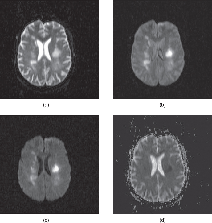
Figure 12.2 Diffusion-weighted EPI sequence: (a)  ; (b)
; (b)  ; (c)
; (c) 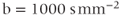 . Normal tissue has moderate diffusion of water, while tissue under stress, such as that at risk for a stroke, has restricted motion of tissue water and shows increased signal on image with significant diffusion sensitivity. (d) ADC map, calculated from images (a), (b), and (c). Low pixel amplitudes indicate restricted water movement. High pixel amplitudes indicate free water movement.
Two approaches are used to address the directional dependence of diffusion. The first approach is to acquire a trace image. This is an image created by averaging the diffusion in a voxel at a chosen  value in three directions. The trace image has the advantage that it is independent of the particular axes used for the measurement as long as they are orthogonal (perpendicular). In other words, the trace image is the same regardless of the gradient direction (invariant). This allows the three primary gradient axes
  to be used. The trace images can provide an estimate of the amount of overall diffusion present in a tissue, but it discards the directional information available about molecular motion.
The other approach for analyzing the directional dependence is to measure the complete diffusion tensor and calculate the preferential directions for diffusion within the voxel. As mentioned above, the preferential directions for diffusion do not necessarily correspond to gradient directions nor macroscopic patient anatomy. To determine these directions, measurements are made with the two gradient pulses in Figure 12.1 having all possible gradient pairs 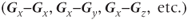 . The measurements made with the gradient directions in the same direction
  will generate the diagonal elements of the tensor while those acquired with the gradient directions being different
 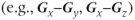 will correspond to the nondiagonal terms of the tensor. Current measurement techniques allow for as many as 256 different gradient direction pairs to be made within a scan. The preferred direction(s) for diffusion can be determined by diagonalization of the tensor matrix (calculating the eigenvalues or characteristic values). The coordinate system that generates the diagonal representation for the tensor
  corresponds to the preferred diffusion directions (eigenvectors or principal axes). The eigenvalues correspond to the ADC along that particular direction.
Use of the eigenvector coordinate system to specify the diffusion directions is frequently used as it provides the simplest representation of diffusion. One common presentation is to display diffusion as a three-dimensional ellipsoid, with the axes of the ellipsoid representing the preferred diffusion directions, and the size of the ellipsoid in a given direction related to the square root of the eigenvalue (ADC) for that direction (Figure 12.3). Isotropic diffusion is represented as a sphere, with equal eigenvalues in all three directions and no preferred direction. Anisotropic diffusion will have one eigenvalue different from the other two or all three eigenvalues different. The first case will have an ellipsoid with two directions equal in length while the second case will have all three axes of different lengths. The principal diffusion direction is the axis with the largest ADC, represented as the longest dimension in the ellipsoid.
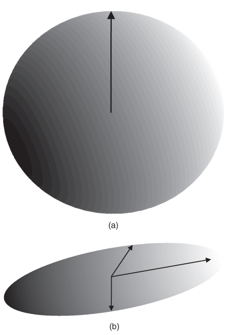
Figure 12.3 Ellipsoids representing principal axes for diffusion. (a) Isotropic diffusion: diffusion is equally likely in all directions and is represented by a sphere. (b) Anisotropic diffusion: diffusion is more likely in one or more directions. The direction that is most likely has the largest vector length.
Another method of analysis of diffusion anisotropy divides the diffusion tensor into two parts, one describing the diffusion that is isotropic  and one containing the anisotropic component
  . Two quantities can be derived from the anisotropic component. The relative anisotropy (RA) compares the magnitude of these two quantities:

while the fractional anisotropy (FA) compares the anisotropy to the diagonal representation:

Both of these quantities are zero if diffusion is isotropic, but FA is used more frequently. Color is also used to represent the different components of the principal eigenvector ( component;
  component;
  component).
One of the most important applications of diffusion-weighted imaging is in the evaluation of cerebral ischemia and stroke. Normal cells maintain a concentration gradient of sodium ions extracellular and potassium ions intracellular, and are surrounded by and contain water. The enzymatic process responsible for the maintenance of this gradient is known as active transport or the sodium–potassium–ATP pump. The energy for this process is provided by adenosine triphosphate (ATP), which in turn requires oxygen as one of the reactants for its production. The oxygen for this process is carried to the tissue from the lungs by erythrocytes as an  –hemoglobin coordination complex. Following the onset of ischemia and the loss of oxygen by the tissue, the ADC of the affected tissue water has been observed to decrease, leading to a decrease in signal dephasing and an increase in signal amplitude (see Figure 12.2). Although the reason for this decrease in ADC is unclear, it is presumably due to a change in the membrane permeability to the sodium and potassium ions and an accompanying increase in intracellular water content. This ADC decrease is reversible upon restoration of blood flow, provided it occurs before complete cell membrane breakdown.
12.2 Perfusion
Although angiographic techniques visualize the vascular network within a patient, they do not have sufficient spatial resolution to visualize blood flow through a tissue in bulk. However, it is possible in many instances to observe changes in tissue signal due to the blood flow through it, a process known as perfusion. Proper tissue perfusion is critical to ensure an adequate supply of nutrients to the constituent cells as well as removal of metabolic byproducts. It also aids in maintenance of a stable tissue temperature. Abnormalities in perfusion can lead to an increased temperature sensitivity and a loss of tissue viability through hypoxia.
Two examples where perfusion studies have shown promise are in the examination of abnormalities of blood flow within tissue and for the detection and characterization of tumors. Blood flow anomalies in the myocardium following infarction have been studied for many years using radionuclide agents. First-pass MR perfusion studies have shown good correlation with these studies and have enabled visualization of different phases of perfusion (Wilke et al., 1999). In these examinations, the measurement parameters are chosen so that the blood signal is minimal prior to contrast agent administration. Reduced uptake of the contrast agent in poorly perfused tissue causes a delay in signal enhancement. Liver studies following administration of gadolinium-based contrast agents have also demonstrated differences in tissue perfusion. Images acquired immediately following contrast administration show capillary phase perfusion, whereas images acquired 45 seconds postadministration show substantial portal phase perfusion (Figure 12.4). The normal spleen usually shows a serpigenous enhancement pattern immediately following contrast administration, with a more uniform signal intensity observed on images acquired 45 seconds or later.
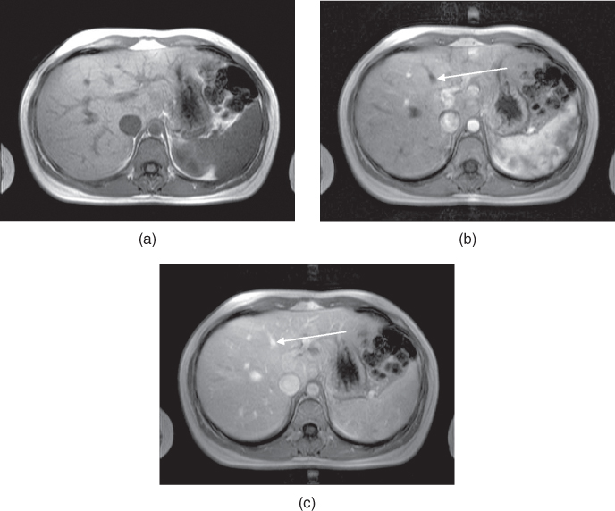
Figure 12.4 T1-weighted two-dimensional spoiled gradient echo imaging of liver following administration of gadolinium–chelate contrast agent. (a) Image acquired prior to contrast administration. (b) Image acquired immediately following administration. Contrast agent is in the hepatic arterial phase, as evidenced by the nonopacified hepatic vein (arrow). (c) Image acquired 45 seconds following administration. Contrast agent is now in the capillary phase, as evidenced by its presence in the hepatic vein (arrow).
The other studies where differential perfusion has been used are in the detection of certain tumors. Pituitary adenomas have demonstrated a difference in perfusion between microadenomas and macroadenomas following contrast administration (Finelli and Kaufman, 1993). Also, malignant breast tumors have demonstrated a significantly faster uptake of contrast media than benign tumors in some studies (Kvistad et al., 2000). Rapid scanning is necessary as both classes of tumors have similar signal amplitudes 3 minutes following contrast administration. Use of a 3D volume scan enables a bilateral breast study with good spatial and temporal resolution (Figure 12.5).
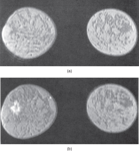
Figure 12.5 T1-weighted three-dimensional volume spoiled gradient echo imaging of breast following administration of gadolinium – chelate contrast agent. (a) Precontrast image, lacking evidence of lesion; (b – d) serial images acquired every 48 seconds following contrast agent administration. Note increased signal from lesion in later images.
12.3 Functional brain imaging
Several aspects must be considered when performing BOLD fMRI studies. Correction for patient movement between measurements must be performed. Also, conversion to a standardized coordinate system is necessary if image comparison between patients (compensating for brain size, shape, and positional differences) and with other measurement techniques (CT, PET) is to be performed. The experimental paradigm or stimulus execution scheme is a critical aspect. Performance of the paradigm by the patient during the examination is of fundamental importance to ensure that the measured activation is a result of the executed paradigm. One approach used to confirm this correlation is to perform the measurements as several sets of paired scans (stimulus present, stimulus absent). The correlation coefficient of the voxel intensity and the time variation of the stimulus is also calculated to ensure that the observed variation is in response to the stimulus. A threshold of significance, known as the z score, must also be defined for the particular study below which the signal difference is assumed not to be relevant. Finally, the pixel intensity from the stimulated image typically exceeds that from the unstimulated image by less than 5%. This necessitates the repetition of the measurement many times (1000 or more) to ensure that the observed signal variation from the voxel is real and not artifactual in origin. High magnetic field strengths (1.5 T or greater) are necessary to increase the change in T2* between activated and nonactivated tissue. The development of scanners with  of 3 T or greater have allowed more reliable and reproducible results to be obtained through an overall increase in SNR.
An important requirement for these examinations is a reproducible, stable performance of the scanner hardware. Deviations in hardware output should be less than 1% over 15 minutes or longer of continuous scanning. This requirement is much more stringent than is required for routine scanning. Environmental factors such as thermal stability of the scanner electronics and building vibrations are two common causes of abnormal signal variations in these examinations.
BOLD-type functional MRI studies have been used for studying many areas of the brain, including the visual, auditory, motor, and frontal cortex. Their results have compared favorably with those obtained using positron emission tomography (PET). Simple stimuli such as flashing lights or finger tapping have been used successfully. More complex stimuli such as cognitive processes (word or picture association) are currently being evaluated.
12.4 Ultra-high field imaging
Note that this section discusses concepts that are more fully explained in Chapter 14.
The development of MR scanners with  significantly greater than 1.5 T presents a number of challenges. While clinically useful images have been demonstrated at field strengths of 7.0 T, commercially available clinical MRI systems are limited to 3.0 T or less. As of this writing, however, scanning at field strengths up to 8.0 T for subjects older than 1 month for research purposes is considered to be of low risk, subject to approval by local institutional review boards. The challenges of so-called ultra-high magnetic field scanners can be divided into two categories: those exclusive of patient tissue and those due to changes in the tissue response to the increased magnetic field.
As might be expected, many of the areas of concern with conventional field strength magnets are also valid with ultra-high field systems, and in some cases of greater concern. For example, current ultra-high field magnets are superconducting solenoidal magnets and use liquid He as the cryogen, as are most conventional magnets. The higher field strengths require greater amounts of magnet wire windings, increasing the overall size and weight of the magnet, and greater amounts of electrical current to generate the magnetic field. The larger  will also exert larger forces of attraction than conventional magnets of the same physical size. This will increase the audible noise of the scanner during measurements. The fringe magnetic field will also extend outside the magnet housing to a greater extent, increasing the influence of the environment on the magnet homogeneity. Shimming of the magnet is also more problematic, in that the absolute inhomogeneity (measured in Hz or
  over a particular distance or volume) increases with increased
  while the relative homogeneity (measured in ppm) might remain constant. Ferromagnetic objects must be kept at greater distances to prevent uncontrollable attraction into the bore. Safe distances for patients with metal implants or for electronic equipment will extend farther from the magnet isocenter. Proper site planning and preparation is critical for safe and successful magnet installations.
As with scanning at conventional  , there are issues with RF power at ultra-high field strengths. As stated in equation (1.1), the resonant frequency
  is proportional to
  . RF penetration is more difficult at higher frequencies, a phenomenon known as the skin effect. This can cause inhomogeneous excitation of a slice, producing shading in images. In addition, increased power from the transmitter is necessary to produce the RF pulses. As mentioned in Chapter 14, the power from a pulse is used in the calculation of the SAR for a scan. The power produced by a pulse is proportional to the square of its frequency, so that increasing
  by a factor of 2 increases the pulse power by a factor of 4. This means that whole-body scanning at ultra-high
  will require different examination protocols in order not to exceed the same SAR guidelines.
There are also tissue response differences to ultra-high  . The net magnetization
  is directly proportional to
  , so that the potential exists to obtain an increased signal. This is particularly beneficial for MR examinations of nuclei other than hydrogen. The absolute chemical shift difference between fat and water hydrogen atoms (measured in Hz) increases linearly with
  , while it remains constant when measured in relative units (ppm). Increased receiver bandwidths will be required in order to reduce chemical shift artifacts to acceptable levels. On a practical basis, the maximum inherent SNR will increase proportionally to
  . This can be exploited in two ways. Smaller voxels can be scanned allowing improved spatial resolution. For example,
 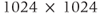 image matrices with excellent image quality can be obtained with acceptable scan times using ETSE sequences. Alternately, MR scans can be acquired with equivalent SNR with fewer signal averages. This can result in shorter scans, allowing better time resolution in dynamic examinations.
There are additional tissue response issues that can have a significant effect on clinical scanning. As mentioned in Chapter 3, the T1 relaxation times increase significantly with increasing  while the T2 relaxation times increase much less dramatically. This means that significant T1 saturation can occur in scans at ultra-high field strengths using measurement parameters that produce minimal saturation at conventional scanners. As a result, longer TR times are necessary to achieve equivalent tissue contrast. This aspect, together with the increased SAR, has limited use of traditional spin echo for acquiring T1 images of the brain or spine. Instead, use of gradient echo is being explored to provide acceptable image quality. There are also increased magnetic susceptibility differences at ultra-high
  . This can produce more severe artifacts in areas where these differences are significant, but can be exploited when performing perfusion or functional MR examinations.
12.5 Noble gas imaging
As discussed in Chapter 1, the most common nucleus observed in MRI is  , due to its high natural abundance and its large nuclear magnetic moment. In spite of these advantages, the net magnetization produced in patients by the
  atoms in water or fat through the Zeeman interaction at normal imaging magnetic fields is very small and induces a weak signal. Other attempts at measuring MR signals from endogenous nuclei such as
  have succeeded, but their low sensitivity has limited their practical implementation.
Successful MRI studies of lung air spaces using hyperpolarized  and
and  gases have been reported (MacFall et al., 1996; Mugler et al., 1997). Visualizing lung air spaces using normal
  imaging is difficult due to low concentration of water in air, large magnetic susceptibility differences due to the paramagnetic nature of molecular oxygen, and artifacts from respiratory or cardiac motion. Although the latter two problems can be minimized using rapid scan techniques with short TE times, the low signal amplitude produced by water vapor cannot. Helium and xenon are noble gases that are relatively unreactive and dissolve into tissues readily. They can rapidly permeate into the lung spaces. They are also well tolerated by most patients, with the most common side effect being a mild sedative effect produced by xenon.
The source of the MRI signal from noble gases is spin polarization between the parallel and antiparallel orientations, just as for any MR measurement, but it is generated in a different manner. Rather than using the natural thermal spin polarization produced by the MRI magnet, these gases are polarized outside the patient through the use of a laser and rubidium atoms. The rubidium atoms are excited by the laser and transfer the energy to the particular gas ( or
or  ). This results in a net magnetization 10,000–100,000 times that produced by the MRI magnet. This hyperpolarized gas is then inhaled by the patient through a ventilator bag. Gradient echo imaging techniques are used to produce images until the net magnetization is completely lost through T2* relaxation (approximately one minute following inhalation) (Figure 12.6).
Figure 12.6  image of normal lung acquired following inhalation of hyperpolarized helium gas. Note significant signal in trachea and upper lobes of lungs and lack of signal from other tissue in the body. Measurement parameters: pulse sequence, two-dimensional refocused gradient echo, postexcitation; TR, 25 ms; TE, 10 ms; acquisition matrix,
  , 128 and
  , 256; FOV,
  . (Reproduced with permission of James R. MacFall, Duke University.)
There are several technical difficulties in performing noble gas imaging. First, the  and
and  active isotopes are not the predominant isotopes for these nuclei (see Table 1.1). For this reason, they are relatively expensive and recovery of the gas following patient studies is performed to reduce the expense. Second, the resonant frequencies for these nuclei are very different from
  so that different transmitter and receiver coils are used from those used in standard MRI studies. Third, noble gas imaging is a single-pass study. Because of the method used to produce the net magnetization, there is no possibility for a repeat measurement following inhalation. Finally, only gradient echo techniques are possible. Spin echoes require 180° refocusing pulses and the recovery of net magnetization through T1 relaxation prior to subsequent excitation pulses. There is no natural regeneration of the net magnetization of hyperpolarized noble gases once it is dephased.