Cisco’s EIGRP (Enhanced Interior Gateway Routing Protocol) is an advanced distance vector protocol based on DUAL (Diffusing Update Algorithm). In this book, we will explain EIGRP’s operation, explore network design, and cover troubleshooting for common problems.
Just in the first paragraph, we’ve introduced concepts that need clarification; we’ve said EIGRP is enhanced and advanced. In this first chapter, we’ll try to clarify these concepts by covering the fundamental workings of EIGRP, keeping in mind that this book has been designed to provide quick answers to common configurations and problems rather than an in-depth study of the protocol. To put EIGRP in perspective, we will first briefly discuss the operation of two prevalent types of routing protocols.
Routing protocols can generally be classified as either distance vector or link state; several well-known implementations of these two types of protocols are common in most networks. In this section, we’ll discuss the basic characteristics of both and present some of EIGRP’s unique traits. A more detailed discussion of EIGRP is presented later in this chapter.
The most common distance vector protocol is RIP (Routing Information Protocol). When someone says a protocol is a distance vector protocol, most people think “periodic updates and slow convergence.” Although some distance vector protocols, such as RIP and Cisco’s IGRP (Interior Gateway Routing Protocol), do converge slowly and use periodic updates, these aren’t the defining attributes of a distance vector protocol.
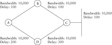
The main characteristic of a distance vector protocol—and what distinguishes it from a link state protocol—is that each node in the network advertises all the destinations it knows about to its directly attached neighbors. This reachability information is announced in the form of a distance—the cost of reaching a particular destination—and a vector—the direction packets should take to reach the destination. In other words, like a sign in the highway, the advertisement indicates the destination, the distance, or cost, to get there, and the direction to take. As with the highway sign, no information is given about the topology of the network, although some clues can be inferred from the number of hops, or the cost. We’ll use Figure 1.1 and walk through how some of this process works.
Updates: If the routers in this network are running a distance vector protocol, they will advertise the information they know to all their directly attached neighbors. Obviously, C would initially be the only router that knows how to reach 10.1.1.0/24. C will advertise this information to B and D, which in turn will advertise it to A—and back to C. When it receives an advertisement, or update, a router increments the metric to reflect the cost of traversing the link between itself and its neighbor. Any paths other than the best path are discarded. Although C receives an update from both B and D that contains a route to 10.1.1.0/24, C discards them because they have a higher metric than the route to the directly connected interface the destination is attached to.
Figure 1.1. A simple network
In RIP and IGRP, the advertisements are periodic, so it will take a multiple of the advertisement interval—90 seconds in IGRP’s case—for information to be propagated across the network. This sounds pretty slow to us! Each router learns the direction toward the destination from the advertising neighbor: Router A can reach 10.1.1.0/24 through either B or D. This algorithm—advertise everything known to all directly connected neighbors and choose the path with the best metric—is known as the Bellman-Ford algorithm.
Periodic updates affect not only the initial information transmission but also the propagation of changes. In some distance vector implementations, after a change is detected, the protocol must wait until the periodic timer expires to advertise the new information.
Furthermore, the network may fall into a count-to-infinity problem in which two or more nodes enter in a routing information loop until the cost reaches the maximum value. In RIP, infinity is reached when a hop count of 16 is arrived at; protocols with a composite metric, such as IGRP and EIGRP, have a much higher concept of infinity. Bear in mind updates are sent—after incrementing the metric—to all the neighboring nodes. As an example, assuming that the cost on all the interfaces is 1, C would advertise the route to 10.1.1.0/24 with a metric of 1, and nodes B and D would advertise the route with a metric of 2.
Consider a failure scenario in which C loses its interface to 10.1.1.0/24; C will still receive updates from B and D with a metric of 2—and in this case, 2 is the best metric! B and D, having lost their best route, will now prefer the metric of 3, advertised by both A and C, and will advertise a metric of 4. Both A and C will now use the route with a metric of 4 as their preferred path and will advertise a metric of 5. This process will repeat itself until infinity is reached. Because the advertisements may be periodic, counting to infinity may take quite a long time. Common techniques aimed at preventing count-to-infinity routing loops are holddown, split horizon, and poison reverse. Later in this book, we will cover specifics on how they affect EIGRP’s operation.
Unlike some implementations of RIP and IGRP, EIGRP doesn’t use periodic updates. Instead, EIGRP uses incremental updates, which means that changes are propagated immediately. The use of incremental updates speeds the initial information transfer and decreases the time for change data to reach the whole network.
EIGRP also doesn’t discard unused path information but instead keeps it in a topology database. DUAL, which is used in EIGRP, uses the information in the topology database to find alternative loop-free paths that will be used in case the main path is no longer present. DUAL and the protocol’s behavior when changes occur are described later.
Metrics: Throughout this book, the terms cost, distance, and metric are used to indicate the same thing. RIP uses hops as its metric; each node in the network represents 1 hop. The maximum number of hops is 16, thereby limiting the size of the network. In Figure 1.1, for example, the distance to 10.1.1.0/24 from A would be 2 hops: through either B or D.
IGRP and EIGRP may use up to four different parameters to calculate the cost: bandwidth, delay, load, and reliability. The following formula calculates the metric in IGRP:
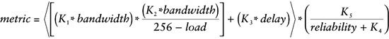
By default, the value for the constants is K1 = K3 = 1, and K2 = K4 = K5 = 0. Furthermore, the bandwidth is the normalized value (with respect to 107) of the minimum bandwidth (in kilobits per second) in the path to the destination. The delay is the sum of the delays (in microseconds) in the path. Substituting these values into the formula and reducing it results in

The use of a composite metric—one made up of more than one variable—allows for having a better criterion for selecting the best path. A higher cost can be assigned to slower paths.
Link state protocols have been considered an improvement to solve some of the problems encountered with distance vector protocols: slow convergence, count to infinity, and so on. OSPF (Open Shortest Path First) and IS-IS (Intermediate System to Intermediate System) are examples of widely deployed link state protocols.
Routers running a link state protocol advertise only their local information but do so to all the other routers in the network. Each router is responsible for announcing information about the state of the links—attached subnets and neighbors—it is directly connected to. The updates are incremental, with a periodic refresh, and are flooded throughout the network by sending them to a multicast address. Each node makes a local copy of the link state packet and forwards it.
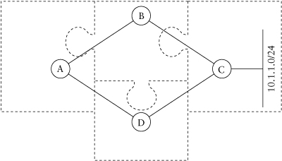
A network implementing a link state protocol can be thought of as a jigsaw puzzle, as shown in Figure 1.2. The link state information that each node originates represents a piece of the puzzle. Once any node has all the pieces, it may calculate the shortest path, or lowest cost, to any given destination.
The flooding mechanism distributes the information, guaranteeing that all nodes receive it. The Dijkstra algorithm is used to calculate a tree—with the local node as the root—from this information and finds a loop-free path to every destination. As you can imagine, this method of finding the shortest path can be very CPU intensive, especially as the
Figure 1.2. A simple network: jigsaw puzzle
size of the tree increases. Link state protocols introduce the concept of areas to reduce the sizes of the trees; areas are network regions that must have the same topology database. Areas represent logical boundaries for the flooding of link state information.
Areas also complicate and limit link state protocols. In general, areas must be built in a hierarchy, and filtering and summarization can be done only at area boundaries or at the node where the information originated. Distance vector protocols—and EIGRP specifically—provide more flexibility by allowing filtering and summarization at any point in the network.
As far as metrics is concerned, OSPF uses the link bandwidth to calculate the cost. IS-IS uses an arbitrary cost.
We’ve covered quite a bit of ground so far. Here’s a short comparison of EIGRP with other protocols on various dimensions.
Algorithm:
• RIP/RIPv2: Bellman-Ford distance vector
• IGRP: Bellman-Ford distance vector
• OSPF: Dijkstra link state
• IS-IS: Dijkstra link state
• EIGRP: DUAL distance vector
Metric:
• RIP/RIPv2: hop count
• IGRP: based on bandwidth and delay
• OSPF: based on bandwidth
• IS-IS: arbitrary cost
• EIGRP: based on bandwidth and delay
• RIP: periodic full updates to a broadcast address
• RIPv2: periodic full updates to a multicast or broadcast address
• IGRP: periodic full updates to a broadcast address
• OSPF: flooding as needed and periodically to a multicast address
• IS-IS: flooding as needed and periodically to a multicast address
• EIGRP: updates and queries as needed to a multicast address
Loop prevention:
• RIP/RIPv2: split horizon and holddown timers
• IGRP: split horizon and holddown timers
• OSPF: full knowledge of topology
• IS-IS: full knowledge of topology
• EIGRP: split horizon and DUAL
Convergence:
• RIP/RIPv2: holddown and wait for alternative paths to be advertised
• IGRP: holddown and wait for alternative paths to be advertised
• OSPF: rerun Dijkstra with modified database
• IS-IS: rerun Dijkstra with modified database
• EIGRP: DUAL, possible use of alternative known loop-free routes or queries to neighbors for alternative-path information
Other features:
• RIP: classful; filtering possible on any router; no summarization within a major network
• RIPv2: classless; and otherwise similar to RIP
• IGRP: classful; filtering possible on any router; no summarization within a major network
• OSPF: classless; filtering and summarization possible on Autonomous System Border Routers (ASBRs) or Area Border Routers (ABRs)
• IS-IS: classless; filtering and summarization possible when a route is injected into the network or at a level boundary
• EIGRP: classless; filtering and summarization possible anywhere in the network
Although the mathematical basis for EIGRP is complex, the protocol is easy to configure and to run in small and large networks. In this section, we walk through neighbor relationships, reliable multicast, and limiting bandwidth consumption. We’ll then look at how DUAL works, the metrics, and, finally, the query process.
EIGRP relies on neighbor relationships to provide reachability information. Having learned information from a neighbor, a router assumes that the information is valid as long as the neighbor relationship stays intact. If the information does change, the advertising neighbor is required to transmit a query, an update, or another indication of the change. In other words, EIGRP has no periodic routing updates.
These neighbor relationships are formed and maintained through hello packets. Each router periodically transmits hello packets to a multicast address on each attached link. Any other router that receives these hello packets will note a new neighbor and will begin the process of advertising routes to it. The first update packet the router sends to this new neighbor will have an initialization bit set, letting the new neighbor know that it needs to start sending back any routing information it has.
If it doesn’t hear a hello from a neighbor within the hold time, a router will assume that the neighbor is no longer there and will remove any topology information received from that neighbor. It is important to mention that the hold timer is reset when any packet—not just a hello packet—from a neighbor is received.
How often are hello packets sent, and how long is the hold time? The answers depend on the link type speed.
• For all point-to-point link types, including HDLC (high-level data link control) serial links, frame relay point-to-point subinterfaces, and others, the hello timer is 5 seconds, and the hold timer is 15 seconds.
• For all links with a bandwidth over 1,000,000 (approximately T1 speed), the hello timer is 5 seconds, and the hold timer is 15 seconds; this category includes all LAN (local area network) media.
• For all multipoint links with a bandwidth less than 1,000,000 (approximately T1 speed), the hello timer is 60 seconds, and the hold timer is 180 seconds.
The hello and hold timers on either end of a link don’t need to match for a neighbor relationship to be built, because the hold time is included in the hello packet itself. A router will use the hold time advertised by its neighbor to determine how long it should wait without hearing any hello packets before declaring the neighbor down.
A routing protocol can send updates and other information between routers in three ways:
• Unicast, which is how BGP (Border Gateway Protocol) works, as well as EIGRP and OSPF in some situations
• Broadcast, which is the way the RIPv1 works
• Multicast, which is the way EIGRP, IS-IS, and OSPF work
Multicast is more efficient than broadcast because the packets can be filtered by most network interface chips rather than being passed up to the IP layer to be sorted. EIGRP uses the multicast address 224.0.0.10, which translates to the MAC (media access control) address 01-00-5E-00-00-0A.
In order to ensure that routing updates and queries are not lost, we need a way to make certain other routers have received these multicast packets intact and to recover from errors if they haven’t. For these reasons, updates and queries are handled by the reliable multicast transport in EIGRP.
Let’s use Figure 1.3 to discuss how the process works. We’ll go through a very simple case, and then we’ll work through a failure scenario.
• A sends out some information that both B and C need to receive. A sends this information to the EIGRP multicast address.
• B receives the information and sends a unicast acknowledgment back to A.
• C receives the information and sends a unicast acknowledgment back to A.
Simple, right? Updates and queries are sent as multicast packets, and the receiving router always acknowledges their receipt, using a unicast packet. What if A sends out a packet, B replies, but C never does? How long would A wait before doing something to recover, and what would A do?
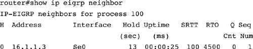
How long will a router wait before starting the recovery mechanism? Each time it sends out a multicast packet that must be reliably delivered, an EIGRP process will wait until the RTO (retransmission timeout) period has passed before beginning a recovery action. This period is calculated from the SRTT (smooth round-trip time), which is
Figure 1.3. Reliable multicast in EIGRP

calculated as the amount of time taken in the past for each peer on an interface to respond.
The values of the SRTT and the RTO depend on quite a few parameters, including the number of neighbors on the interface, the number of retransmissions attempted, and the bandwidth configured on the interface. As these parameters vary dynamically, so does the formula to calculate the SRTT and the RTO. In the simple case of two neighbors on a point-to-point interface, the RTO is typically six times the SRTT; the value may vary from a minimum of 200 microseconds (ms) to a maximum of 5 seconds (s). These timers are shown in the output of the show ip eigrp neighbor command.
How does the router recover from a failed multicast? If a router sends out a multicast packet and never receives an acknowledgment, what action does the router take? First, the router makes a list of all the neighbors from which it did not receive an acknowledgment. Second, the router sends out a packet telling those neighbor routers that didn’t respond not to listen to multicast until they’ve been notified that it’s safe again: that recovery is complete. Third, the router will begin sending unicast packets with the information to the routers that didn’t answer, continuing until they’ve caught up.
Let’s work through a more practical example, using the network depicted in Figure 1.3 as an example.
1. A sends out an update or a query, a type of multicast packet that must be delivered reliably.
2. B responds with an acknowledgment, but C doesn’t respond.
3. A waits for the neighbor for the period of time specified in the RTO.
4. Once this time period has passed, A sends out an unreliable-multicast packet, called a sequence TLV (type-length-value) packet, which tells C not to listen to multicast packets any longer.
5. A then continues sending any other multicast traffic it has and delivering all traffic, using unicast packets to C, until it acknowledges all the outstanding packets.
6. Once C has “caught up,” A will send another sequence TLV, telling C to begin listening to multicast again.
Steps 4 and 5 are repeated until node C has received all the outstanding information. The sequence TLV packet contains a list of the nodes that should not listen to multicast packets while the recovery takes place. The packet sent in step 6 does not contain any nodes in the list.
While recovering, each reliable multicast packet transmitted has the CR (conditional receive) bit set to indicate that it should be processed only if the receiving node’s address was not present in the preceding sequence TLV packet. The CR bit is also useful if node C can receive multicast packets only intermittently; the CR bit guarantees that the node will not process the reliable-multicast packet if the sequence TLV packet was not received.
How long will the router continue attempting to recover from a failed reliable multicast? Once a router drops back into unicast transmissions, it won’t keep trying forever to get the information transmitted. A router will either (1) attempt to retransmit the unicast 16 times, waiting longer to try again each time it retransmits or (2) continue to retransmit until the hold timer for the neighbor in question expires. Once it has been sending retransmissions for the longer of these two periods of time—16 retries or the hold time for the neighbor—a router will declare a retransmission limit exceeded error and will reset the neighbor.
What is transmitted using reliable multicast? The types of packets that warrant the attention the reliable-multicast system provides are updates and queries. Hellos, acknowledgments, and sequence TLVs are sent unreliably; that is, they don’t require acknowledgments.
One of the problems facing protocols that send routing information only on demand is that they can consume all the bandwidth available exchanging routing information while trying to converge. EIGRP resolves the problem of bandwidth starvation by consuming only up to 50 percent—the default value—of the bandwidth available on a link. (The amount of bandwidth that EIGRP is allowed to consume is configurable.)
EIGRP accomplishes this by pacing its packets. Essentially, the process is:
• Calculate how long it takes to send a single bit on the link.
• Multiply that number by the size of the packet ready to be sent.
• Wait this amount of time—or a portion/multiple of this time, depending on the configuration—before sending the packet.
What bandwidth is used for the calculation of this pacing interval? Again, it is the bandwidth that is configured on the interface. Refer to Table 3.1 for a list of the default bandwidths for some common interfaces on Cisco routers.
It’s always best to manually configure the bandwidth for what the line rate really is—or the committed information rate for links that have a clock rate different from the signal rate—rather than just use the default. This is particularly true for serial links, which almost always default to 1.544 and almost always have a lower real bandwidth. On multipoint (not broadcast) interfaces, the bandwidth available is divided by the number of neighbors reachable through the interface, to compensate for the lower link speeds that are likely at the remote ends of the links.
The foundation of EIGRP is the Diffusing Update Algorithm, or DUAL, a method of finding loop-free paths through a network, proposed by J. J. Garcia-Luna. We will discuss the theory behind DUAL before diving into how EIGRP has implemented it.
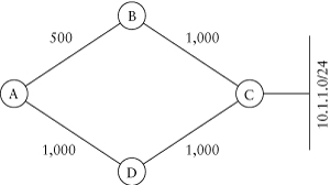
The fundamental concept behind DUAL is as follows: It is mathematically possible to determine whether any route is loop free, based on the information provided in standard distance vector routing. In other words, DUAL can determine which path to a destination is loop free, in a way that is independent of choosing which path to use. Let’s go into a practical example, based on Figure 1.4.
Assume that A is trying to find the best path, or lowest cost, to 10.1.1.0/24. A traditional distance vector protocol, such as RIP or
Figure 1.4. A simple DUAL example
IGRP, would simply add the cost of each link and choose the best path. The remaining paths would be discarded because the protocol assumes that worse paths are possible loops and should be avoided. It’s clear from Figure 1.4 that A has two loop-free paths available: one through B and the other one through D.
Using the following process, DUAL will quickly determine that these two paths are both valid:
• Compare the cost of the two paths and select the lowest; this cost is called the feasible distance (FD). The neighbor advertising this path to the destination becomes the successor. The total cost of the path is obtained by adding the cost to reach the neighbor—1,000 to reach node D from node A, for example—to the metric advertised by that neighbor.
• The metric advertised by the successor is called the reported distance (RD), or the distance the neighbor is reporting to the router performing DUAL. In this case, the reported distances through B and D are both 1,000.
• In any case, where the reported distance (RD) is less than the feasible distance (FD), the path is considered loop free. Any neighbor that meets this criterion becomes a feasible successor (FS).
It is mathematically provable that any path with an RD that is less than the FD will be loop free, but we’ll leave that as an exercise for the reader.
With these basics in hand, we can begin to look at how EIGRP implements DUAL. The metrics are integral to the remainder of the discussion, so let’s approach them first.
As discussed earlier, EIGRP builds on the metrics used in IGRP. The basic information used to build the EIGRP metric is provided by the bandwidth and the delay, and the formula used to compute the metric is

One question that often arises when people see the formula is: Why multiply by 256? Wouldn’t it be simpler just to compute things as they are? Well, yes. But remember that EIGRP uses the IGRP metric as its reference point and that IGRP uses a 24-bit number—224 is its maximum metric—to represent the distance to a destination. EIGRP’s designers wanted to use 32 bits to add granularity to the metric. The simplest way to use the 32 bits was to shift the existing IGRP metric left by 8 bits, which is equivalent to multiplying it by 256.
Although EIGRP also keeps the path MTU (maximum transmission unit), link reliability, and link load in the topology table and can be configured to use this information when calculating the best path, none of these other metrics can trigger an update, so they aren’t very useful. In other words, EIGRP will not recalculate the best path based on the load of the links in the path alone: Something else must change to prompt EIGRP to recalculate the path metric before it will notice that the load on the path has changed. We would recommend, therefore, that the other metrics shouldn’t ever be used, and we won’t discuss how to use them.
When advertising a destination, EIGRP uses bandwidth and delay as they are configured on the router’s interface. In other words, the delay is not measured in real time or anything like that. The value assigned to the delay depends on the default bandwidth on the interface (see Table 3.1 for some sample values). The delay can also be configured independently of the bandwidth, using the interface-level delay command.
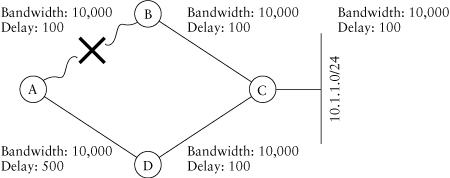
Figure 1.5 shows the same network as in Figure 1.4 but this time with a little more realistic metrics assigned to the links. Let’s use this network to determine what router A would have in its topology table and what happens when one of the two paths to the network attached to router C fails.
The first thing to do when figuring out which path A will choose is to see what metric A will calculate for each path.
• The path through B will be ((107 / 10,000) + 100 + 100 + 100)256, which is 332,800.
• The path through D will be ((107 / 10,000) + 200 + 100 + 100)256, which is 358,400.
So A will choose the path through B as the best path and will route traffic in that direction. Now, will A believe that the path through D is loop free? Let’s calculate the RDs to see.
Figure 1.5. A simple network, using real metrics

• The RD from B will be ((107 / 10,000) + 100 + 100)256, which is 307,200.
• The RD from D will be ((107 / 10,000) + 100 + 100)256, which is 307,200.
Is the RD through D less than the FD (the metric through the best path)? Yes, 307,200 is less than 332,800. So A will believe that the path through D is loop free and will mark it as a feasible successor (FS) in its topology table.
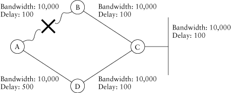
Let’s take a look at what A will do if the path through B fails (Figure 1.6). When the link fails between A and B, router A will immediately recognize that its best path to the network attached to C is no longer valid and will search its topology table for another loop-free path to this destination. Because A has another loop-free path, the path through D, A will begin using this path.
So far, we’ve dealt with a very simple case: two paths, one of which is an FS of the other. In reality, few cases are this simple, and we have to contend with split horizon.
Split horizon is the rule that a router should not advertise a path to a destination through the interface it is using to reach that destination. (Let’s call this interface the upstream interface.) Split horizon is used in all
Figure 1.6. Losing the best path in the simple network
distance vector protocols to speed convergence. The theory behind split horizon is as follows: There’s no need to advertise the cost to the destination in the upstream direction, because the cost should be higher. In other words, the upstream routers should already have a lower-cost path available. In many cases, the use of split horizon in distance vector protocols reduces the convergence time by avoiding the count-to-infinity problem.
EIGRP also uses split horizon. In some cases, it may contribute to DUAL’s not finding an alternative loop-free path, even if one exists. Let’s modify our simple network slightly to provide an example in which split horizon has an influence on DUAL (Figure 1.7).
Let’s begin with D rather than A, as that’s where the action is this time. D will compute
• The path through A as ((107 / 10,000) + 100 + 100 + 100)256, which is 332,800
So D will choose the path through A as its successor. Computing the RDs, we find that
• The RD from A is ((107 / 10,000) + 100 + 100)256, which is 307,200.
• The RD from C is ((107 / 10,000) + 100)256, which is 281,600.
Because 281,600, the RD through C, is less than 332,800, the FD, or the best path, the path through C will be marked as an FS in D’s topology
Figure 1.7. A simple network with split-horizoned routes
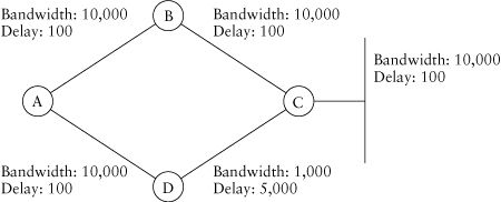
table. Because D is using the path through A, D will not advertise that it can reach the network attached to C toward A; it will apply split horizon to it. A will have only one path to the network attached to C: through B.
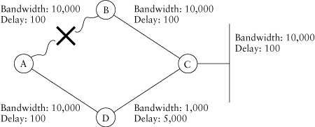
Let’s look at what happens if the path between A and B fails now (Figure 1.8). When the link between A and B fails, A finds that it has no other path to the destination network. In other words, node A does not have a feasible successor in its topology table. How does A find the valid alternative path? When a topology change occurs, EIGRP actively searches for an alternative path to any destinations impacted by the change. EIGRP searches for alternative paths by sending query packets to all its neighbors, asking them whether they know of a different path to the destination. The query process allows EIGRP to converge quickly in many circumstances, but it can also create significant activity if a serious trauma occurs. (More details on how to avoid or minimize problems are presented later in the book.) In steady state, all entries in the topology table are marked as passive; during the query process, affected routes are marked as active. Queries are sent to all the neighbors except the ones that advertised the active route.
A will send a query to D, which will examine its topology table and discover that although it has now also lost its best path, it does have another loop-free path, an FS, through C for this destination. D will reply with this information, and the network will converge with the path through D as the only path. It is important to mention that if node D didn’t have a feasible successor, it would also send a query to all its neighbors (except A, in this example).
Figure 1.8. Convergence in a network with split-horizoned paths
Although we’ve presented a simple case in which queries come into play, there are other cases. Changing the metrics in the sample network, we could make it so that A uses B as its primary path, D uses C as its primary path, but the path through D doesn’t appear to be loop free from A’s perspective (Figure 1.9).
Let’s calculate the metrics and RDs as A sees them.
• The path through B has a metric of 332,800 and an RD of 307,200.
• The path through D has a metric of 409,600 and an RD of 358,400.
Because the RD through D is higher than the best path, the FD, the path through D is not considered loop free and is therefore not marked as an FS in A’s topology table. From D’s perspective,
• The path through A has a metric of 384,000 and an RD of 332,800.
• The path through C has a metric of 358,400 and an RD of 281,600.
So the path through A is a feasible successor, with the best path being through C. Note that D is not using the path through A, so it will not split horizon; it will advertise the destination network to A.
In this situation, if the link between A and B fails, A will examine its topology table and find that it knows another path. A suspects that the alternative path contains a loop, so it will mark the route active and will query its neighbors for other paths to the destination.
Because D is using the path through C as its best path (successor), it will reply to A with the metric for the path through C. Once A has
Figure 1.9. Queries with no feasible successor
received replies for all its queries, it will see that C has replied with a valid alternative path and will begin using it. In Chapters 3 and 4, we present an in-depth analysis of issues that have to be taken into account for the successful completion of the query process.
Queries may cascade throughout a network, stopping only when one of three conditions is met:
• An alternative path is found.
• The end of the network is reached.
• Information about the network that is the subject of the query is unknown.
When it receives a query, a router may give three answers.
• If it receives a query about a route and has an alternative path that doesn’t go through the router asking the question (a feasible successor), a router will immediately answer with the metric it uses to reach the target. It doesn’t need to send queries to anyone else, because it has no need to search for another path; it already has one.
• If a router receives a query and has no one else to ask, it immediately replies with an answer of infinity or unreachable, meaning the destination isn’t reachable through this router.
• If a router receives a query about a route not contained in its topology table, it immediately answers with an infinity reply or unreachable.
The last property is extremely important to understand when designing an EIGRP network and is the subject of much of the discussion presented in Chapter 3.
When it sends a query to its neighbors, a router sets a timer for approximately 3 minutes (it could be as high as 3º minutes) and must receive replies to all queries before the timer expires. If the timer expires, the route is considered SIA (Stuck in Active), and the peering with the neighbor that didn’t answer is reinitialized. However, reinitialization of the neighbor relationships is not something you want to happen regularly on your network. Occasional SIA routes will happen on most EIGRP networks of significant size and are not any reason to be alarmed. SIA routes are, however, an indication of problems on the network; if they happen too frequently, SIAs will greatly reduce a network’s stability.
Probably the most frequently asked question for not only EIGRP but also any protocol is: What protocol should I use in my network? What protocol is best? The answer to these and similar questions is very simple: It depends!
Some of EIGRP’s main traits that should be considered when selecting a protocol for your network are
• Cisco-proprietary protocol
• Classless protocol
• Filtering and summarization possible at any point in the network
• Distance vector protocol
• Incremental updates
• Query process used to find alternative paths
This list is in no way an indication that if any or all of these characteristics can be accommodated, you should use EIGRP in your network; it’s just a short summary of things to keep in mind when making your decision.
You will find that EIGRP has some strong points and some weak ones, as any protocol used for carrying routing information does. There is no “silver bullet” in the world of routing protocols, just good design coupled with choosing the right tool for the job. In many large networks, EIGRP performs quickly, puts minimal strain on the network, and allows a great deal of flexibility.