EIGRP has proved itself a flexible, reliable protocol if it’s used in a network that has been designed with stability in mind. If you just let an EIGRP network happen, without proper design considerations, however, it can easily be a nightmare to manage and to maintain. In this chapter, we discuss EIGRP network design issues, including techniques to improve your network and pitfalls to avoid. Throughout this chapter, we will build on the concepts presented in Chapter 1. We will briefly cover some fundamental questions you must consider in order to build a scalable, reliable network. We will then discuss specific design issues and suggested techniques.
Before we start discussing specific situations you will face when building an EIGRP network, we should start with the foundation of it all. A network that “evolves” without consideration being given to hierarchy and address summarization is unlikely to remain stable as it grows. Some of the strengths of EIGRP also lead to its vulnerabilities; unless you design EIGRP networks to avoid these vulnerabilities, reliability will be negatively impacted.
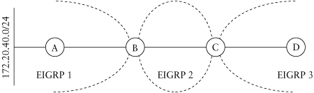
As the previous chapters describe, EIGRP converges extremely quickly when a change in the network occurs. This rapid convergence results from the manner in which EIGRP searches for an alternative path when the topology changes. Instead of waiting for periodic updates to advise the routing protocol of changes, EIGRP will energetically look for an alternative path if a change in the topology occurs.
When EIGRP actively pursues an alternative path to a destination, every router that could provide an alternative path is interrogated until EIGRP finds one or runs out of routers to ask. This process, known as the query process, is explained in detail in Chapter 1. Several techniques can reduce the number of routers involved in the query process, but almost all of those techniques require a hierarchical network topology and addressing that provides for summarization. The importance of using these techniques will be made clear later in this chapter.
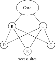
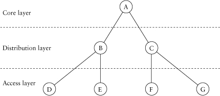
Typically, the hierarchy should reflect at least three layers: core, distribution, and access, as shown in Figure 3.1. Although the three-level hierarchy may not be appropriate for every network, it is an excellent place to start. In this model of hierarchy, the network’s core layer comprises high-powered routers whose job is to switch packets as quickly as possible. No functions that degrade packet switching, such as access control or policy application, belong in the core of the network.
The distribution layer is attached to the core and uses the core to pass traffic between the access layer of the network and common access services, such as server farms and Internet access, and other locations in the distribution/access layers. The distribution layer is responsible mainly for traffic aggregation and route summarization. The distribution layer is also where WAN (wide area network) links would be connected to the core of the network.
Figure 3.1. A simple hierarchical structure
The access layer is typically the point where users are attached to the network. Access routers are normally the least-expensive and lowest-powered routers in the network, with much lower traffic-switching performance requirements. The access layer is intended to provide access to the network to one, or at least very few, groups of users. The access layer is also where access control and policy application are performed. For example, if quality of service were used on the network, traffic classification and policing would most likely occur at the access layer.
Why is hierarchy important for EIGRP’s stability? The well-defined roles of the various layers provide an excellent method of determining where route summarization and information hiding can be performed. In the next section of this chapter, we’ll discuss information hiding and its importance. But remember: Without hierarchy, these extremely important tools cannot be used successfully.
Another aspect of the physical topology that needs to be considered is the level of redundancy required in order to meet the service-level requirements of the network. Redundancy is a necessary part of every network design: Failures happen, and a design that won’t tolerate failure is a poor design. A network that works only when every piece of it works won’t survive in the real world; redundancy must be designed into the network from the ground up.
Excessive redundancy can be worse than no redundancy at all, however. When a topology change occurs, EIGRP searches every available path—within certain limits, which we will cover later in this chapter—in order to look for an alternative, working path. When there are apparently dozens of alternative paths from a router to every destination, the amount of work required to investigate each alternative can be overwhelming. When designing a network, you should determine the level of redundancy required to provide fault-tolerant service to network users and eliminate every other path from EIGRP’s list of alternatives.
One common example of excessive redundancy is two or more routers connected through numerous user segments, typically via switches and VLANs. The networks connecting these routers are intended to provide access for users (or to services) connected to them, rather than alternative transit paths through the network. By transit
Figure 3.2. Multiple parallel user segments

traffic, we mean traffic not originating or terminating on a segment but flowing through the segment while traveling across the network. Figure 3.2 shows an example of excessive redundancy owing to user VLANs with routing enabled.
In order to reduce this excessive redundancy across these user segments, you should evaluate every link and determine which ones are intended to provide a routing path for transit traffic. Any segment not intended as a transit path should be removed from the EIGRP topology by applying the passive-interface command under the router process for each interface to be removed. For example, for the network depicted in Figure 3.2, you would configure the following:
router eigrp 1
passive-interface FastEthernet1.1
passive-interface FastEthernet1.2
. . .
The results would be the greatly simplified topology depicted in Figure 3.3.
In summary, without proper hierarchy, information hiding cannot be performed, and your EIGRP network will be susceptible to instability unnecessarily. How can you improve stability once you’ve created a hierarchical network with reasonable redundancy? The following sections should provide you with some insight.
Figure 3.3. Simplified topology

To review, if a router loses a route, such as when an interface goes down or an update is received from a neighbor withdrawing a route, or the metric to a destination has increased (become worse) and doesn’t have another equal-cost path (alternative successor) or feasible successor, it sends queries to all neighbors except those connected through the interface used to reach the destination. When a router receives a query from a neighbor that was previously the successor for a given destination, and it doesn’t have any alternative successors or feasible successors, the router will send its own query to its neighbors, asking them whether they know an alternative path, and so on.
In this manner, a chain of queries cascades throughout the network, stopping only when one of the following conditions is met:
• An alternative path is found.
• The end of network is reached.
• Information about the network that is the subject of the query is unknown.
In most networks of significant size, the queries may not be answered from time to time, generating Stuck in Active routes. Occasional SIAs should not be a concern, but frequent ones are. How do we minimize SIA routes? We do so by decreasing the number of routers and links involved in the query process. We call this action minimizing the query scope in a network. How do we minimize the query scope? Referring back to the three ways in which queries cease to be propagated, we can
• Always have unaffected alternative paths to all destinations in the network. This goal is a laudable target but hardly realistic. Remember: Excessive redundancy is bad.
• Make the end of the network happen sooner rather than later. If your network is small enough, you probably won’t have SIA problems. Of course, it seems that every network is increasing in size, not decreasing, so this approach isn’t a very realistic one, either.
• Make the network referenced in the query unknown. This is the answer!
If you use information hiding in order to make the paths unknown on a large part of the network, you will minimize the number of routers involved in convergence. Consequently, you will be decreasing the convergence time and, more important, the odds of getting Stuck in Active routes.
Two techniques are available that easily hide information in EIGRP networks. The flexibility of these techniques is one of the primary factors that make EIGRP a widely deployed routing protocol on large networks. By using these techniques at strategic places in the network, EIGRP will scale very well and will remain reliable in large networks. Its flexibility is far greater than that of its two primary competitors among modern routing protocols, IS-IS and OSPF. The two techniques are route summarization and route filtering.
First, we’ll look at route summarization in an EIGRP network. Summarization for EIGRP networks has two forms. Although they are implemented quite differently, the overall impact on the query range is the same. Which technique you need to use is based on how your IP addresses are assigned.
The first type of summarization you will encounter in EIGRP is autosummarization. EIGRP automatically performs summarization at major network boundaries unless you explicitly shut it off with the command no auto-summary. With autosummary enabled, any router configured with multiple network statements—routers that attach to more than one major network—will automatically send only a summary route on the major network boundary, suppressing all the network components. For example, in Figure 3.4, router A has several interfaces on the 10.0.0.0 network and several interfaces on the 172.16.0.0 network. With autosummary enabled, EIGRP will summarize all the 10.x.x.x components into a single route, 10.0.0.0/8, to send out all the 172.16.0.0 interfaces. Likewise, EIGRP will advertise only the 172.16.0.0/16 destination instead of the individual components through all the interfaces in the 10.0.0.0 network.
Figure 3.4. Autosummarization
Of course, this technique can be used only at major network boundaries, limiting its usefulness. Autosummary should be disabled only when discontiguous subnets are within your network, because discontiguous networks require the propagation of all components to all routers. A discontiguous network is one in which not all the components of a major network can be reached via links that are also part of the same major network. Although discontiguous networks are a reality, they are not a recommended design choice. See Figure 3.5 for an example of a discontiguous network.
In addition to autosummarization, EIGRP also supports manual summarization, which is much more administratively difficult but also far more flexible than autosummarization. Manual summarization lets you suppress routes and advertise a summary for those routes on any interface in the network. This flexibility permits you to do multiple levels
Figure 3.5. A discontiguous network
of route aggregation—difficult or impossible with IS-IS or OSPF—and allows the network’s physical hierarchy to define where summarization should occur.
Remember the discussion on network hierarchy at the beginning of this chapter? A hierarchical network gives us natural points in the network to do summarization, assuming that the network addressing was also performed in a manner permitting it. In Figure 3.6, the addressing has been done with summarization in mind, allowing you to aggregate addresses on each distribution-layer router toward the core. The result of summarization is that all the destinations attached to the access routers for a single distribution router can be represented by a single route. In this case, all the destinations reachable through router B can be represented by the single route 10.1.0.0/16, and all routes reached through router C can be represented by 10.2.0.0/16.
As mentioned earlier in this chapter, the key ingredient to making EIGRP more stable and scalable is to hide information. If fewer routers have knowledge of a particular destination, fewer routers will be involved in convergence when the destination’s state changes. With summarization, we are hiding the information by aggregating the component routes into one or more summary routes. Only the summary is known beyond the summarization point; the components are unknown.
Using Figure 3.6 as an example, if the interface on router D for 10.1.1.0/24 goes down, router D will send a query to router B, looking
Figure 3.6. Summarization in a hierarchical network

for an alternative path. When router B receives the query, it will look in its topology table, not find an alternative path, and generate a query toward router A. When it receives the query, router A will check its topology table and will find that it also doesn’t have an entry for 10.1.1.0/24 but instead has only the summary route 10.1.0.0/16. Because it doesn’t have 10.1.1.0/24 in its topology table, router A will immediately send a reply to router B, reporting that it doesn’t have an alternative path to 10.1.1.0/24, and the query process will be completed.
As described in Chapter 2, manual summarization is configured on each interface of a router through which a summary route should be sent. This makes the implementation of manual summarization a bit more administratively burdensome. To perform manual summarization, you must first decide where routes can be aggregated in your topology. In our example, using Figure 3.4, the job was made simple through the use of a hierarchical topology and intelligent address assignment.
Filtering routes in EIGRP is another very useful technique for information hiding. In this section, we’ll describe how the two techniques differ in function and will give an example of when a route filter is a better choice than summarization.
When you summarize manually or through the autosummarization process, EIGRP creates a summary route with an administrative distance of 5 with a next hop of the interface Null0 and advertises the summary out the appropriate interfaces. All the components of the summary are filtered automatically, so only the summary is received downstream. Performing summarization creates the aggregate route and removes the components in one step.
With route filtering, on the other hand, no routes are created. The only function performed by route filtering is eliminating routes from being sent or received. Why would you want to use route filtering instead of summarization? The most common use is when the route created by the summarization causes a conflict with a real route. For example, summarizing to the default route (0.0.0.0/0) will create a local route to 0.0.0.0/0 through the Null0 interface, with an administrative distance equal to 5. If a real default route is received by the router with the summary configured, it will be rejected because it has a worse administrative distance than the summary route created locally. The results could be disastrous!
Instead of summarizing to 0.0.0.0/0, we can filter the routes sent to the remote routers so that only the 0.0.0.0/0 route is sent. The filtering is done via the distribute-list <number> out <interface> command. Of course, if you decide to use this technique, you should ensure that the 0.0.0.0/0 route will always be received by the router that is filtering to just the default route.
Ensuring that 0.0.0.0/0 is always sent to the remote routers is generally done by defining what is known as a floating static route on the distribution-layer routers, to back up the default route learned from the exit point of the network. It wouldn’t be very good if the 0.0.0.0/0 route injected for Internet access were to disappear owing to link failure or another reason, causing the only route used by the access router to reach all target networks, both internal and external, to disappear and to strand the users attached to access-layer routers!
To implement floating static routes, you enter the desired static route command with an administrative distance value associated with the route: ip route 0.0.0.0 0.0.0.0 10.1.1.1 250, for example. The administrative distance of 250 tells the router to prefer any dynamically learned route to this static one. If the dynamically derived route disappears, use the floating static route. By making the administrative distance of the static route worse than any dynamically derived route, you will use the static route in the routing table only if the dynamically derived route disappears.
Another example of route filtering as a better approach than summarization is when you want to limit the routes sent through an interface to a subset of the all known routes but don’t want to limit it to only the summary. In Figure 3.7, for example, a remote site is connected to two distribution routers, one in New York and one in San Francisco. For most traffic coming from the remote sites, it doesn’t matter whether the path through New York or San Francisco is used.
Summarization, however, would produce suboptimal routing. If only the 10.0.0.0/8 entry or a default route is sent from the distribution routers B and C, the remote router wouldn’t know which path to take to reach the components of 10.1.0.0/16. As a result, router A could send some traffic destined to New York through router C!
Figure 3.7. Route filtering
A more appropriate approach would be to put route filters in place, permitting only 10.0.0.0/8 and the subnets located in New York to be advertised from router B and only 10.0.0.0/8 and subnets located in San Francisco to be advertised by router C. Of course, if the 10.0.0.0/8 route doesn’t exist in the network, you must define a local static route—typically to null0—and redistribute it into EIGRP. You would probably want to filter this redistributed static route to prevent other distribution-layer routers from learning about it.
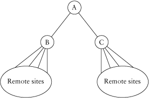
Defining a router as a stub means that it is used only to attach user segments to the remainder of the network via one or more paths. Figure 3.8 gives an example of a situation in which defining a router as a stub is useful.
In Figure 3.8, three access sites, D, E, and G, are connected to the distribution layer via two serial links each. These sites, known as dual-homed remotes, are intended to provide reliable access to the remainder of the network for the users located at the remote sites. Although the dual legs could provide an alternative path for traffic from the distribution layer through the remote and back to the distribution layer, this behavior isn’t what was intended. Configuring each of these remote routers as stubs tells EIGRP that they are not intended to be a transit path for network traffic traveling from one distribution router to another.
Figure 3.8. Stub networks
When the remote router is defined as a stub, it will advertise only local routes: connected, static, or summary. This means that any route learned from one distribution-layer router will not be advertised back out to the other distribution-layer router. We can provide this function with distribution lists, but defining the router as a stub router automatically causes this route filtering to happen.
Additionally, and more important, when a router is defined as a stub router, the distribution-layer routers know that they will never find an alternative path through the stub router and thus will never even send queries toward the remotes. This is a major advantage because it now removes all the stub routers from the query process entirely. The distribution lists mentioned earlier block updates but not queries; if the remote routers are not defined as stubs, queries will continue to flow to them.
Some network administrators decrease the query scope by defining multiple autonomous systems and redistributing among them. Although this approach may make EIGRP vaguely resemble OSPF with its area hierarchy, it doesn’t contain the query scope as expected. When a query reaches the end of an autonomous system, a reply to the query is indeed sent back. Unless summarization or route filters are implemented, however, a new query will then start up in the next autonomous system. It’s as if the query were given new life!
Some network administrators have successfully implemented multiple autonomous systems with the heavy use of route filtering and summarization. Given political or administrative reasons to make different portions of the network different autonomous systems, it may be a good way to implement this separation. However, it isn’t helping to minimize the query scope.
Query scope can also be decreased by removing from the EIGRP topology links and routers that don’t need to be running EIGRP! For example, if an access site has a single path into the rest of the network and the link to the site is of poor quality, you should consider removing it from EIGRP. Configure a static default route on the remote router to provide a path for the traffic from the remote, and configure a static at the distribution-layer router that provides a path to the destinations at the remote. Redistribute the static routes at the distribution-layer router into EIGRP so the rest of the network has the information it needs to reach the remote destinations. This is a drastic measure but is sometimes the best approach to take.
Another approach gaining in popularity is to use ODR (on-demand routing) to get the routes from the access sites into the distribution layer and then to redistribute those ODR routes into EIGRP. ODR routing takes advantage of the CDP (Cisco Discovery Protocol), which advertises the interface addresses of each router to its directly connected neighbors. The addresses advertised are limited, however, to the primary interface addresses. If a router has static routes, secondary addresses, or any other source of routes, ODR will not propagate them.
In summary, numerous tools and techniques are available for decreasing the query scope of an EIGRP network. It is vitally important for you to evaluate the various methods of containing the convergence process to the area of the network where it is necessary. Evaluate each of these techniques and choose the ones that make the most sense in your network. If your addressing will not permit summarization and your topology is nonhierarchical, you may need to consider changing some of the basic structure of your network. If you don’t make wise choices in your topology and addressing, you will be fighting an uphill battle. If you don’t use the information-hiding techniques available to you, your network stability will be in jeopardy.
In this section, we discuss various aspects of path selection in EIGRP networks. (See Chapter 1 for an explanation of the metric components.) Here, we’ll deal with design issues associated with changing metric parameters (bandwidth and delay) on an interface, changing the K value, variance, asymmetrical routing, and default routing strategies. We will start by discussing modifying interface metric parameters to influence the path EIGRP chooses to a given destination.
Sometimes, you’ll want to change the next hop chosen through the normal metric calculation/path selection process in EIGRP. If the next hop for some but not all destinations through a particular path need to be influenced, it’s best to use route maps to influence only those routes rather than changing interface information, which influences the path chosen for all destinations.
If all the routes through a particular next hop need to be influenced, however, the natural method of modifying the path selection is to change one of the components used in the metric calculation to make the routes more or less desirable. The choice then becomes which parameter should be changed. As explained in Chapter 1, normally only two parameters are used in the metric: bandwidth and delay. Because both bandwidth and delay can be modified on a single interface, which should you change to modify path selection?
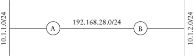
Let’s take it one parameter at a time. What is typically called the bandwidth parameter in the metric is the minimum bandwidth in the path to the target network. On the router doing the metric calculation, the smallest bandwidth between it and the target of the route is included in the bandwidth portion of the metric calculation. By modifying the bandwidth parameter on an interface, you may or may not be changing the metric for a particular route!
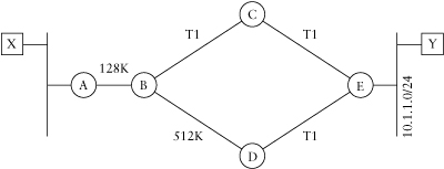
In Figure 3.9, the minimum bandwidth to network 10.1.2.0/24, from router A’s point of view, is the T1 (1.544 Mbps) between it and router B. If you decreased this bandwidth value to 512Kbps in order to influence path selection, the metric for 10.1.2.0/24 would indeed change. However, the minimum bandwidth to network 10.1.4.0/24 is 128K, the lowest-speed link to 10.1.4.0/24 from router A. So the change made between router A and router B in order to influence path selection had absolutely no impact on the metric for the route to 10.1.4.0/24!
EIGRP also uses the bandwidth configured on an interface to determine the pacing interval between EIGRP packets. If you change the bandwidth parameter to influence path selection, you may be changing pacing intervals to such an extent that the convergence of the network will be put in jeopardy!
For example, if you changed the bandwidth statement on an interface to be 1Kbps, in order to make a path a backup route—normally not preferred in EIGRP’s routing decisions—you would inadvertently leave EIGRP with only 0.5Kbps to send all its updates, queries, and replies! This bandwidth is probably not enough to even have the neighbor relationship between routers successfully be established! Obviously, changing the bandwidth value can have consequences far beyond those intended.
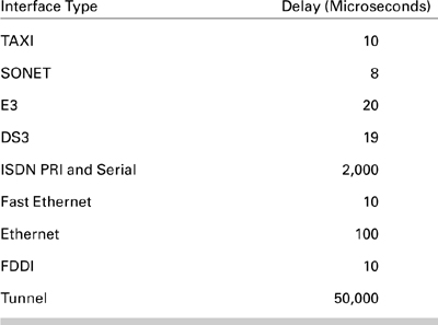
Delay is the other parameter you can use in order to influence path selection. Table 3.1 lists some of the default delay values for each interface type. These default values can also be overridden on each interface, using the delay command. The delay values are cumulative, so from a router doing the metric calculation, all delays between it and the target network are added to arrive at the delay value in the metric. The delay on the outbound interface of the router toward the target is included.
Figure 3.9. The effect of changing the minimum bandwidth

Table 3.1. Default Delays by Interface Type
Because the delays for each link are added to arrive at a total, modifying the delay value on a link will almost certainly change the metric of all destinations reachable across this link. It is possible, although unlikely, to set the delay value high enough so that a minor change to the delay will not change the overall, or composite, metrics. This behavior is possible because of the way the delay value is stored internally. The display of the delay value on the interface is in microseconds, and the command is entered in tens of microseconds. Therefore, if the value shown by show interface is 20,000 and you want to increase the delay to 25,000, the interface configuration command would be delay 2500.
Path selection can also be impacted with the offset-list command, which you can use to tell EIGRP to add extra delay to updates received from or delivered to a particular neighbor. Furthermore, the offset list can be used with an access list to define a subset of routes to apply the additional delay to. In this manner, you can easily select which routes will be influenced by the command.
For example, if you wanted router A in Figure 3.10 to prefer the path through router C for packets destined to network 10.1.4.0/24 but
Figure 3.10. Offset lists
would prefer the remainder of the destinations go through router B, you would use the following offset list to accomplish the purpose:
hostname A
!
router eigrp 100
offset-list 10 in 100 serial 1
!
access-list 10 permit 10.1.4.0 0.0.0.0
One additional tool that can be used to influence path selection in an EIGRP network is to change the K values used to determine the weight of each element in the total metric calculation. The K values can be changed so that EIGRP uses additional elements, such as the reliability of a link, in the metric calculation. Also, the K values can be changed so that EIGRP acts more like RIP, treating the delay as a hop count through the network.
It’s often tempting to use some of the other metric attributes that EIGRP includes in its metric calculation beyond the defaults (minimum bandwidth and total delay), but before embarking on this course, you need to understand the significant limitations. The additional parameters that can theoretically be used to determine path selection include load, reliability, and the minimum MTU along the path.
At first glance, using load or reliability to determine which path should be used seems a reasonable—even desirable—design idea. For example, if a particular path is congested (load is high) or having physicallayer errors (reliability is low), it would be nice if the routing protocol would avoid using it. To accomplish this dynamic rerouting around poor or overloaded links, you might want to change the K values so the load and reliability compute into the metric. But although this change may be logical, it’s not useful.
Unlike IGRP, which sends periodic updates and can also use reliability and load in the metric calculation, EIGRP sends updates to its neighbors only when the topology changes. Unfortunately, a change in load or reliability isn’t considered a topology change, so a change in either load or reliability will not cause an update to be sent. This makes enabling the K values for load or reliability relatively useless.
For example, the load on a link could increase dramatically, yet a router running EIGRP will not notify any of its neighbors of the changed load value even if the K value for load is enabled. If an update is sent owing to a topology change, the higher load will be reflected in the update, so the neighbors would then learn about the busy link.
Of course, if traffic is diverted owing to the metric change with the high load and the load drops significantly, again a router running EIGRP will not notify any of its neighbors of the change. A fairly underutilized link will continue to be avoided, based on the state of the link when the last update occurred, not the current state of the link. Only on the next topology change causing an update would neighbors learn of the new conditions of the link.
So, changing the K values to pay attention to load or reliability of a link is not very useful. What about the other changes some people make to the K values? Sometimes, you might want to minimize the number of router hops taken to any destination and thus want to change EIGRP’s behavior to more closely resemble RIP’s normal behavior. In other words, you may want to base routing decisions on hop count instead of the lowest metric calculated from the minimum bandwidth and total delay. How can you do this? If you eliminate the K value for bandwidth and manually define all the delay values so they are the same on all interfaces of all routers in the network, you will end up with a hop count–based routing protocol.
Variance changes the path selection process by permitting routes with unequal costs to be installed in the routing table, thus allowing the router to load share over multiple unequal-cost paths in proportion to their metrics. Normally, EIGRP and all routing protocols will default to installing up to four equal-cost paths in the routing table. With variance, EIGRP goes beyond equal-cost paths and permits unequal-cost paths to be installed. Even so, EIGRP still guarantees that each route installed in the routing table will be loop free by allowing only feasible successors to be installed.
Figure 3.11 shows two paths from router A to network 10.1.1.0/24. The link from router A through router B is significantly better than the path from router A through router C and will be, by default, the only route installed in A’s routing table, leaving the path through router C idle. Because you probably don’t want to see links you are paying for idle, you can use variance to change the default behavior of installing only the best route in the routing table.
By adding the command variance 2 under the router EIGRP process, EIGRP will use the variance value as a multiplier to the best metric—feasible distance through the current successor—to determine which other routes should also be included in the routing table. In the network in Figure 3.11, router A’s metric for network 10.1.1.0/24 through router B is 6,500, and through router C is 10,000. With the variance set to 2, EIGRP will multiply the route through router B by 2 and then compare it to the metric through router C. Because the cost of
Figure 3.11. Variance across unequal-cost paths

the path through router C is lower than the cost of the path through router B, owing to the multiplier, the path through router C is also installed in the routing table.
You might think that using variance could cause congestion problems on the link between router A and router C, as we’ve made the path through router C appear equal to the path through router B, which is, in fact, a better route. Couldn’t this cause more traffic to use this path than it can handle? EIGRP is smart enough to realize that the variance statement didn’t change the capacity of the links and will send traffic from router A to router C path proportional to the variance. In other words, traffic will be apportioned to the links, based on the metrics toward the destination.
As not too much traffic will be sent over the lower-bandwidth link, it sounds like a fine plan. Can any alternative path be used to load share with the variance command? No. The alternative path must also meet the feasibility condition, which was explained in Chapter 1. It’s logical that you shouldn’t use an alternative path to load share if it may introduce a routing loop. By meeting the feasibility condition, the loop-free nature of the alternative path is ensured.
Does using variance have any drawbacks? Unfortunately, the answer is yes. You must keep two issues in mind before deciding to use variance in your network: its global scope and the possibility of packets arriving out of order.
In the preceding example, variance was used to solve a single problem—using all the available bandwidth from router A to network 10.1.1.0/24. By configuring variance, this problem was solved. What isn’t so obvious, however, is that the variance multiplier is now used on all routes in the topology table. Even if a single destination is the desired target of the change, the impact to other routes could also be felt, whether desired or not. It is impossible to limit the scope of variance.
The second possible problem introduced by the use of variance is the very real possibility of out-of-order packets. Some IP stacks are more tolerant than others about receiving out-of-order packets; the overhead involved in reordering out-of-order packets may be significant in some cases. In fact, it’s possible that the performance lost through reordering out-of-order packets at the end systems more than negates any gains realized through the load sharing across the less desirable link.
Most modern stacks should tolerate out-of-order packets fairly well, but you should be aware of the possibility of creating additional work for the end systems before deciding on variance as a tool to use. Beyond this, some switching modes within a Cisco router will produce very few out-of-order packets even when variance is configured, such as fast switching and CEE (Cisco Express Forwarding). One other consideration when attempting to load share across links—whether they are equal cost or unequal cost—is that the type of switching used on the router will greatly affect how much load sharing you can achieve, such as which fast-switching routes are cached on a per destination basis. If most of the traffic has only one destination, most of the traffic will end up traversing one link at a time, regardless of how many equal-cost paths exist.
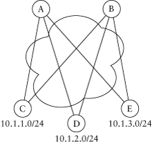
Asymmetric routing means that the path between two particular hosts on a network may be different in each direction. You may think that the routers are acting incorrectly, but in reality, they are acting as expected. In the following example, we will demonstrate this principle.
In Figure 3.12, host X sends router A packets destined to host Y on network 10.1.1.0/24. When it receives a packet, router A will evaluate the alternative paths in its routing table to reach host Y. Because it has only a single path to reach 10.1.1.0/24, router A forwards the packet on to router B, which then evaluates its paths to reach 10.1.1.0/24. From router B’s viewpoint, the best metric to reach 10.1.1.0/24 is through router C, because the minimum bandwidth to reach 10.1.1.0/24 is 1.544Mbps, but the minimum bandwidth is 512Kbps through router D.
On the return path, router E sees two equal-cost paths to reach host X because the 128Kbps link between router A and router B is the minimum bandwidth for both paths back to host X through both router D and router C. Because the delay values are the same on each interface—delay for a serial link defaults to 20,000—both paths appear to have equal metrics, and router E load shares between them.
Figure 3.12. Asymmetric routing
As this example shows, the path chosen in each direction is independent. You shouldn’t count on the path to a target being reflected in the return path.
If, where, and how to originate the default route for the network also needs to be thought out when considering path selection through the network. A default route is used to provide a path for a router to send packets to if the destination address of the packet is unknown and is often used to provide a routing path to external destinations, such as the Internet, and for hiding information.
The most common reason for propagating a default route throughout your network is to provide a path to external destinations. For instance, it isn’t necessary to carry the entire Internet routing table into EIGRP or any other interior gateway protocol when probably only one or two carefully controlled points will exit out of your network toward the Internet. Instead, it makes more sense to carry one route, a default route.
This strategy also carries an element of the second reason for using a default route: information hiding. You can go further than hiding the Internet’s routing table from routers in your network with a default route, though. For example, in Figure 3.13, router B doesn’t need to know about every possible remote site reachable through router C.
Router B needs to know only that if it doesn’t know how to reach a destination, it can simply forward the traffic on to router A. This is a perfect design in which to use a default route to reduce the amount of
Figure 3.13. Hiding information with default routes
information routers B and C and the routers behind them must work with when a topology change occurs.
Once you’ve decided to use a default route, what are your alternatives for generating and propagating it? You can use two strategies, each with many variations. The first alternative is to use a default network statement at one or many places in the network. The second alternative is to use a true default route (0.0.0.0/0).
The Default Network: The default network is an approach left over from the IGRP days. IGRP had no way to represent the default route (0.0.0.0/0) in the IGRP packet, so an alternative strategy had to be created. The method Cisco selected was to allow you to create a default network via the global command ip default-network <address>. The destination address defined using the ip default-network command is flagged in the IGRP and EIGRP updates as a candidate default route.
When it receives a route marked as a candidate default, a router flags it in the routing table: Look for a * beside the route. The best candidate default route is chosen as the default network, and the next hop toward the default network is chosen as the gateway of last resort. All this information can be seen by using the command show ip route.
router>show ip route
Codes: C - connected, S - static, I - IGRP, R - RIP,
M - mobile, B - BGP
D - EIGRP, EX - EIGRP external, O - OSPF, IA - OSPF
inter area
N1 - OSPF NSSA external type 1, N2 - OSPF NSSA
external type 2
E1 - OSPF external type 1, E2 - OSPF external type 2,
E - EGP
i - IS-IS, L1 - IS-IS level-1, L2 - IS-IS level-2,
* - candidate default
U - per-user static route, o - ODR
Gateway of last resort is 10.1.50.8 to network 192.168.20.0
10.0.0.0/24 is subnetted, 1 subnets
C 10.1.50.0 is directly connected, Serial0
C 10.1.14.0 is directly connected, Ethernet0
E* 192.168.20.0 via 10.1.50.8
Although this method of default routing is not necessarily intuitive, it works pretty well.
The Default Route: The default route is another name for the route with all zeros in its address and mask—an address of 0.0.0.0 and a prefix length of 0. This route is typically introduced by a static route defined as
ip route 0.0.0.0 0.0.0.0 [<next-hop>|<interface>]
This static route is then redistributed into EIGRP, using the command
router eigrp 100
redistribute static
default-metric 10000 10 1 255 1500
Remember that IGRP is not capable of representing a default route in its update packets, so IGRP cannot propagate a default route learned from a static route or other source. EIGRP doesn’t have this restriction, however. In our example in Figure 3.13, the natural place to put a static default route is router A. Router A would then distribute a default route so the rest of the network would use the path to it as the way to reach any destination address not in the routing table.
One word of caution, however: in earlier versions of Cisco IOS, Cisco routers defaulted to classful routing. While routing in a classful environment, a router assumes that knowledge of one subnet within a major network implies knowledge of every subnet within a major network. To see why this is a problem, look at Figure 3.14.
Let’s assume that both routers B and C are configured for classful routing and that router A is passing only a default route out to them (0.0.0.0/0). If it receives a packet destined to 10.2.1.1, router B will examine its routing table and find that it knows about some parts of the 10.0.0.0/8 network (components of 10.1.0.0/16) but not this destination in particular.
Router B will assume that 10.2.1.1 does not exist and will drop the packet. If it is configured for classless routing, using the ip classless command, router B will ignore the classful routing rules and will forward the packet along its default route (or best supernet), toward router A.
Default Network or Default Route? Which strategy should you use: default network or default route? If you are still running any IGRP in your network, you must use the default-network strategy. It wouldn’t work very well to use a default route, then lose the ability to propagate this default anywhere in the network running IGRP.
Because you can define the default network on multiple routers in the network when using a default network, you aren’t reliant on a single or a few default origination points. The disadvantage of using the default-network approach is that it takes time to converge on a change in the path to the default network. A process that looks for changes in the gateway of
Figure 3.14. Classful routing

last resort runs every minute, so it may take up to a minute to reconverge on a new default network once the topology has changed.
With the default route, the convergence on a change in the path to the default route will be as fast as any other EIGRP route. It can be significantly faster than convergence using the default network. A disadvantage of using the default route is that it is difficult to inject it in multiple places in the network, so the network is reliant on maintaining a path to the point where the static is redistributed into the network.
We’re now going to change directions a little by focusing on some specific areas you need to consider in order to build and maintain a stable EIGRP network. One of the more troublesome parts of most networks is the wide area network (WAN) links. These links typically have low bandwidths and low reliability and are the cause of many instability problems in EIGRP. In this section, we will discuss several considerations for WAN links and strategies that will increase the EIGRP stability across these links.
One potential problem EIGRP may face with frame relay links is that the rate at which the router connects to the link is not necessarily the rate at which EIGRP can reliably deliver packets. In Figure 3.15, for example, the access rate for the connection to the frame relay network
Figure 3.15. A hub-and-spoke network

on router A is T1 (1.544Mbps), but the access rate from router B is 64Kbps. Additionally, frame relay service providers may provide a CIR (committed information rate), for each connection, defining the data rate the provider will guarantee to deliver across the link. Any traffic that exceeds the CIR value is subject to being discarded in the frame relay network. In Figure 3.15, the CIR for our example link is 32Kbps.
Why should EIGRP care about the available delivery rate on the link? If it is sending updates, queries, or replies across a link, EIGRP should reasonably expect that the traffic it is sending will be delivered to the remote end. Because routers normally try to send data on a link as quickly as the physical link will accept it, EIGRP’s packets would leave router A at 1.544Mbps into the frame relay cloud. Even if the traffic made it across the frame relay network at this rate, it can be delivered to router B only at 64Kbps. However, because the CIR is only half that rate, much of the traffic would probably be discarded in the cloud, anyway!
As EIGRP is most likely going to be sending large amounts of updates, queries, or replies during times of network instability, the worst thing to happen would be if the packets used to converge on the network changes are themselves being dropped. Regaining network stability would definitely be in jeopardy.
In order to avoid this problem, EIGRP uses the defined bandwidth value to determine how quickly it could send EIGRP traffic to its neighbors. The bandwidth value on the interface is now used to define the pacing interval EIGRP will use to put gaps between packets to ensure that it will not overwhelm the intervening network. By default, EIGRP will not use more than 50 percent of the defined bandwidth for reliable packets (updates, queries, and replies). This percentage can be changed on a per interface basis, using the command ip eigrp <AS> bandwidth-percentage <percent>. Later in this section, we will explain why it may be desirable to change the bandwidth percentage.
For this pacing improvement to work, however, you must manually define the bandwidth values on each frame relay interface/subinterface. Although it seems to be laborious, it is necessary to make EIGRP behave correctly on frame relay networks. The results are worth the effort! In most of the following discussion, we refer to frame relay networks, but the principles also apply to other technologies, such as SMDS (switched multimegabit data service), ATM (asynchronous transfer mode), and ISDN/PRI (integrated services digital network/primary rate interface).
Frame relay networks have primarily two scenarios, and each has its own requirements for defining the bandwidth. These two scenarios also have some variations, but the principles are the same. In the next section we will discuss the differences in defining bandwidth in point-to-point subinterfaces and multipoint interfaces/subinterfaces.
With point-to-point subinterfaces, it’s very simple to determine how to implement the bandwidth statement correctly. Each point-to-point subinterface should have the bandwidth set to the CIR value of the PVC (permanent virtual circuit)—DLCI (data link connection identifier)—mapped to the subinterface. If the frame relay PVC has 0 CIR, the bandwidth should be set to something less than the lowest access rate of either end of the PVC. In other words, the bandwidth should be set to a value that describes the data rate EIGRP should reasonably expect will be available for it to use. As mentioned earlier, EIGRP will use no more than 50 percent of this bandwidth value for its reliable packets.
Oversubscribed networks will require you to modify this approach slightly. If the total of all the CIR values exceeds the access rate at the hub of a hub-and-spoke network and if you set the bandwidth to the CIR for each subinterface, EIGRP will believe, falsely, that it has more bandwidth available than it truly has. In other words, do not let the aggregate bandwidth value of all subinterfaces combined on an interface exceed the access rate of the interface.
Sometimes, for network management performance reports to be correct, the bandwidth value may need to reflect the CIR value for each subinterface instead of the decreased value set owing to oversubscription, as mentioned previously. If the aggregate bandwidth values exceed the access rate in this case, you should use the ip eigrp <AS> bandwidth-percentage <percent> statement, as described in Chapter 2, to tell EIGRP to use less than 50 percent of the defined bandwidth.
For multipoint interfaces/subinterfaces, determining the correct bandwidth value to define is a little more complicated. With the point-to-point subinterfaces described earlier, each subinterface connects to only one neighbor; therefore, the defined bandwidth should reflect whatever data rate one can expect to deliver to the neighbor reachable over the subinterface. On multipoint frame relay interfaces/subinterfaces, however, this is not the case.
By definition, a multipoint frame relay interface/subinterface can have many PVCs connecting to many neighbors, all reachable through the same interface or subinterface. The main interface is always a multipoint interface. Because numerous neighbors are normally reachable through the multipoint interface, EIGRP does not use just the defined bandwidth to determine the pacing interface for each neighbor but instead divides the bandwidth value by the number of neighbors to determine the pacing interval for each neighbor.
For example, if the network in Figure 3.15 is using a multipoint subinterface from router A to the four remote routers instead of the point-to-point subinterfaces described earlier, the bandwidth value on the frame relay interface would have to change. EIGRP would look at the defined bandwidth on router A’s frame relay interface and divide it by 3, and then take 50 percent of the resulting value as the maximum amount of EIGRP traffic it can send to any one neighbor. Therefore, when defining the bandwidth value on a multipoint interface/subinterface, you should multiply the CIR values for the remote routers by the number of neighbors in order to determine the bandwidth value.
But what if the remotes have significantly different CIRs? If the PVC from router A to router C had a CIR value of 512Kbps and the other two have CIR values of 64Kbps, what value would you use at the hub? In this case, you multiply the lowest CIR value by the number of neighbors to reach the proper bandwidth value. Although it may constrict the EIGRP packet delivery unnecessarily to the higher-CIR neighbor, it will at least ensure that the lower-CIR neighbors will not be overwhelmed.
An even better idea for multipoint interface with highly disparate CIR rates for neighbors is to split the interface into multiple subinterfaces. In our example, the 512Kbps CIR neighbor could be put on its own point-to-point subinterface, and the bandwidth for the remaining two neighbors could then be properly defined to reflect the expected date rate.
So far, our context has been frame relay interfaces, but the principles also apply to other pseudoshared networks, such as ATM and SMDS interfaces. Similar to frame relay, ATM can have multipoint and point-to-point subinterfaces, and the same pacing requirements exist if the bandwidth is T1 or less. If the bandwidth is greater than T1, the pacing function is turned off.
With SMDS interfaces, another problem we often encounter is that sites connecting to the SMDS cloud may have vastly different access rates, resulting in conditions similar to the ones you might find on a hub-and-spoke frame relay network. Sites with very high access rates into the network can easily overwhelm sites with much lower access rates.
ISDN PRI interfaces using dialer groups or dialer lists also present significant challenges for configuring interface bandwidths. In this case, each ISDN BRI (basic rate interface) dialed in becomes a neighbor on a shared network, which appears to EIGRP as a multipoint interface. So, can we just apply the techniques defined earlier for multipoint interfaces to PRIs? Unfortunately, the answer is no.
With frame relay multipoint interfaces, you have a very good idea of how many neighbors you can expect to see through the multipoint interface. With an ISDN PRI, this isn’t the case. One neighbor could be dialed in, which would mean that a bandwidth value of 64Kbps would be appropriate, or 24 neighbors could be dialed in, which would require a bandwidth value of 1.544Mbps. A dialer group could span multiple PRIs and could have 24, 48, or even more neighbors dialing into a single dialer interface! What a quandary!
The two approaches to resolving this issue are (1) don’t use dialer interfaces or (2) make the bandwidth setting unimportant. Instead of using dialer groups, you can use dialer profiles, so each remote site dialing in is verified by PAP/CHAP and then associated with a virtual interface based on its identity. The bandwidth statement will be applied against each profile, not against the entire dialer group. Virtual templates can also be used in the same manner.
The second approach is to make the bandwidth value less of a factor by filtering the routes sent across the link to such an extent that any bandwidth available is enough to support it! Typically, the filtering is done via a summary-address statement or distribute-list, so that only a default route or one or more major network routes are allowed across the link. By permitting a very few update packets to be sent across the link, the amount of bandwidth available to move it is not as significant a problem. Since dialup connections—even via ISDN—are very limited in their bandwidth, limiting the amount of routing updates across the link is a good approach in any case.
Another issue you will need to consider when designing a network is minimizing the complexity by eliminating the reflection of routes through dual-homed remotes. In many networks, remote sites are connected via two frame relay PVCs—or other technology, but frame relay is the most prevalent—to the distribution layer. Figure 3.16 shows an example of dual-homed remote connection between remotes (routers C, D, and E) and the distribution routers (routers A and B).
Typically, the remote routers are given two PVCs to provide resiliency in the event of a PVC or router failure. The reason for two links to router C and the other remotes is so EIGRP can circumvent a failure of router A, router B, or either of the two PVCs connecting them to router C. Additionally, the two PVCs may be provided for load sharing of traffic from each remote site back to the distribution layer.
What is typically not intended for these two links is to use the remote routers (C, D, and E) for transit traffic. For example, traffic at the distribution layer can be routed from router A to router C and then back down the other leg to router B for delivery elsewhere. Although it
Figure 3.16. Dual-homed remotes
is possible, it is most likely not desirable or intended. Unfortunately, EIGRP has no idea what you intended; instead, it sees only what paths are possible and takes all of them into consideration when routing convergence is required.
This result exhibits itself when a routing update is sent from router A to router C; router C will turn around and readvertise the route back to router B. Likewise, when an update is received on router C from router B, router C will be a good neighbor and send it on to router A. If you look in the topology table on router A and router B, using the command show ip eigrp topology all-links, you will see topology table entries for each target network through every one of the remote sites!
Although EIGRP doesn’t have a problem sorting out the correct path, all of the unused, undesired alternatives must be taken into account in the convergence process when there is a topology change. This process can become time-consuming and ugly. Two general strategies can rectify this situation:
• Limiting through ignorance what is known on the remote
• Filtering the reflection itself
In the first case, you can put summary-address statements or distribute-lists on the distribution routers so the remote routers aren’t receiving the component routes to reflect. The remote routers would then reflect only the summary or limited route set permitted by the distribute-list, decreasing the complexity for the majority of the routes in the network.
The second method is a little more administratively tiresome but is probably the better method for retaining full functionality on the remote routers and limiting the reflection of routes. On each remote, a distribution list would be defined, limiting its routing advertisements on the WAN links to include only the routes that are local to the remote site. In other words, define which subnets must be advertised by a remote router to provide reachability to the resources at the remote site, and permit only these subnets in the routing updates. This is done by a distribute-list out globally or per interface and stops the advertisement of any routes learned from one distribution router from being reflected to the other distribution router.
As an example, let’s return to Figure 3.16, which shows several remote routers with their dual-homed connections. In order to keep router C from reflecting the routes learned from router A, such as 10.1.1.0/24, 10.1.2.0/24, and so on, back to router B, router C would put in the following command:
router eigrp 1
distribute-list 1 out
!
access-list 1 permit 10.1.1.0 0.0.0.255
This means that router C will be allowed to advertise only routes beginning with 10.1.1.0, which will stop it from advertising routes from one distribution router to another.
Another approach to providing service to dual-homed remotes is to use EIGRP stub network support. With stub networks, the remote router would be able to advertise only connected, static, or locally originated summary routes toward the distribution routers. This approach will automatically stop the remote router from reflecting routes from one distribution router to the other.
A third approach to supporting dual-homed remotes is the use of CDP-based on-demand routing (ODR) for getting the remote subnets into the distribution routers, then redistributing these ODR routes into EIGRP at the distribution layer. One limitation with this approach is that ODR will advertise only directly connected primary interfaces. If secondary addresses are defined or if redistributed or dynamically derived routes from the remote site need to be advertised, this approach will not work.
Another situation to avoid arises from the relationship between low-speed NBMA (nonbroadcast multiaccess) networks and SIA routes. As described in Chapter 1, SIA routes occur when a route goes active, one or more queries are issued trying to find an alternative path, and not all replies are received. How do low-speed NBMA networks play a part in this situation?
First, what is an NBMA network? As the name implies, an NBMA network supports access from multiple routers at the same time but doesn’t support broadcast packets. For example, frame relay multipoint networks allow a single IP subnet to be shared by multiple routers in a partial or full mesh topology. Although each router shares an IP subnet with the other routers across the frame relay cloud, they cannot send a single broadcast packet and have it simultaneously delivered to all the other routers on that subnet. Instead, the pseudobroadcast packets would need to be replicated and sent to each neighbor independently.
The challenge in using a low-speed NBMA network involves the timing of retransmission timeouts. As explained in Chapter 1, the default hold time for high-speed, point-to-point, or broadcast-based media is 15 seconds, or three times the hello interval of 5 seconds. For low-speed NBMA networks, such as frame relay multipoint, X.25, and SMDS, the default hold time is 180 seconds, which is three times the hello interval of 60 seconds. This 3-minute hold timer can create a problem in a network because it is the same value as the SIA timer.
Figure 3.17 shows an example of a network containing a low-speed (T1 or less) NBMA network (frame relay multipoint). When the Ethernet on router A fails, router A sends a query to its neighbors, looking for an alternative path to reach 10.1.1.0/24. In our example, assume that we are also having a problem with packet delivery to router D, which is a remote site on a multipoint frame relay link.
Router C will continue to retransmit reliable packets to router D 16 times and then wait until the hold time period has expired. In other words, router C will send the same updates over and over again, for 3 minutes. Then router C will declare router D down, owing to retransmit limit exceeded. In the meantime, however, the query originated from router A would be queued behind the update packets in router C and not complete before the 3-minute period has expired. Because it
Figure 3.17. Low-speed links and SIAs

takes 3 minutes to declare the neighbor down, router A can be waiting those same 3 minutes for the replies to its queries. Thus, router A’s SIA timer will also expire, and the neighbor relationship between routers A and B will be reset.
If the link between routers C and D were to have a lower hold time, the neighbor relationship between them would have been declared down prior to the SIA timer expiration on router A. When it reinitializes router D, owing to the retransmit limit exceeded, router C will send the infinity reply back to router B, saying that it doesn’t have an alternative path to 10.1.1.0/24. Router C terminates the active condition, assuming that all other replies were also received, and the SIA between routers A and B never would have occurred.
Now that we’ve pointed out the problem that low-speed NBMA networks can cause, what can we do about it? Does this mean that you cannot have these types of interfaces in your network? Although point-to-point subinterfaces more closely relate the true topology to EIGRP and eliminate these types of problems, multipoint interfaces may be the best network type for some implementations. Instead of banning point-to-multipoint links from the network, two alternatives exist to avoid the timing problem.
First, you can increase the active timer via the command eigrp timers active-time <time in minutes> so the retransmission timeout will expire on low-speed multipoint interfaces before the active timer. This is not a recommended solution, because EIGRP will delay converging until the active timer expires in the event of a problem on the network.
The second, and preferred, solution is to decrease the hello interval and hold time on low-speed NBMA networks to 30-second (instead of 60-second) hellos and 90-second (instead of 180-second) hold times. Don’t forget to change both! Changing only the hold time without changing the hello interval will almost certainly cause neighbor instability. The commands to change these timers are:
interface s0.1 multipoint
ip eigrp 1 hello-interval 30
ip eigrp 1 holdtime 90
Like all distance vector routing protocols, EIGRP uses split horizon to prevent temporary routing loops while converging. The split-horizon rule states that a router should not advertise destinations out the interface it is using to reach those destinations. For example, in Figure 3.18, the link between routers A, B, and C is a multipoint frame relay network in a hub-and-spoke topology. The hub router, router A, would receive network X from router B but would not advertise it back out to router C, as its next hop is through the same interface.
If you wanted to allow router A to ignore split horizon and to advertise the routes it has learned from router B to router C, you might think that the command no ip split-horizon configured on router A’s multipoint serial interface would change the behavior. In fact, it doesn’t impact EIGRP operation at all! Instead, you must use the EIGRP-specific command no ip eigrp <AS> split-horizon instead. Normally, disabling split horizon is not recommended, but occasionally, a legitimate need for disabling the default behavior occurs.
As frame relay is not broadcast capable, multipoint interfaces duplicate broadcast packets so that each remote attached to the hub router can receive a copy. Quite often, the default broadcast queue will not be large enough to handle the broadcast traffic presented to the interface, and some of the broadcasts will be dropped. As EIGRP packets can be lost because of lack of space on the broadcast queue, the network can become completely destabilized as EIGRP neighbors continually reset.
You can tell whether the broadcast queue is a problem by looking at the output of a show interface and evaluating the field highlighted in
Figure 3.18. Split horizon and multipoint interfaces

boldface type in the following sample output. If a significant number of broadcast queue drops are seen on the frame relay interface, tuning the broadcast queue would be an appropriate step.
Serial 0 is up, line protocol is up
Hardware is MK5025
Description: Frame Relay link to Albany DLCI 100
MTU 1500 bytes, BW 1024 Kbit, DLY 20000 usec, rely
255/255, load 44/255
Encapsulation FRAME-RELAY, loopback not set,
keepalive set (10 sec)
LMI enq sent 7940, LMI stat recvd 7937, LMI upd
recvd 0, DTE LMI up
LMI enq recvd 0, LMI stat sent 0, LMI upd sent 0
LMI DLCI 1023 LMI type is CISCO frame relay DTE
Broadcast queue 64/64, broadcasts sent/dropped
1769202/1849660, interface broadcasts 3579215
The command used to change the broadcast queue is:
frame-relay broadcast-queue size byte-rate packet-rate
The broadcast queue has a maximum transmission rate (throughput) limit measured in both bytes per second and packets per second. The broadcast queue is given priority when broadcasts are being transmitted more slowly than the maximum and therefore has a guaranteed minimum bandwidth allocation. The two transmission rate limits are intended to avoid flooding the interface with broadcasts. The limit is considered reached if the limit for either bytes per second or packets per second is reached. Given the transmission rate restriction, additional buffering is required to store broadcast packets.
The queue size should be set to avoid loss of broadcast (or multicast) routing update packets. The exact size to define depends on the number of packets required for each update. To be safe, the queue size should be set so that one complete routing update for each neighbor can be stored. As a general rule, start with 20 packets per DLCI. The byte rate should be less than both of the following:
• N/4 times the minimum remote access rate, measured in bytes per second, where N is the number of DLCIs to which the broadcast must be replicated
• One fourth the local access rate, measured in bytes per second
The packet rate is not critical if the byte rate is set conservatively. In general, the packet rate should be set assuming 250-byte packets. The defaults are 64 queue size, 256,000 bytes per second (2,048,000 bits per second), and 36 packets per second.
One of the more complicated aspects of designing any network is defining backup strategies. It’s seldom acceptable for a remote site to lose connectivity to the core of the network in the event of a link or a router outage. As mentioned earlier, remote sites need to have resilient, redundant connections to the distribution layer, and many networks use dual-homed frame relay PVCs to meet this need.
However, what happens if both frame relay links are down or the router providing access to those links is down? An alternative path must be provided. Therefore, most people create dial strategies to support temporary connections from remote sites lasting only for the duration of the outage of the normal connection path. Two of the many possible strategies that can be used are
• Dial from remote: If the remote site routers lose all connectivity through their normal links to the distribution-layer routers they are attached to, they would dial in to a router someplace else on the network.
• Dial from distribution: If the distribution-layer router loses all its routing information to a given remote destination, it dials into a router at the remote site.
Beyond deciding which end of the link should initiate the dial backup connection, you must also decide what specific mechanism will be used to start the call. Here again, two options are available.
Interesting traffic: Losing routes causes a floating static route to be installed, which then causes traffic to begin flowing over a dial-on-demand link. Once the router with the dial link begins receiving packets that must traverse the link, that router dials through to the other end so it can forward the traffic.
• Dialer watch: A dialer watch is a specific mechanism used by Cisco IOS to dial a backup link when a primary link fails.
All these configurations deal more with configuring dialup links, so we won’t cover them here. One point of particular interest in an EIGRP network, though, is how the protocol reacts when both the primary link and the dial backup link are connected. In the network depicted in Figure 3.19, for example, the link between routers A and B has failed, causing the backup link between routers C and D to be brought up. After a period of time, the link between routers A and B is repaired. Let’s look at what happens after the link is repaired. Assume that router A is summarizing the routes it learns from routers B and E to 172.20.0.0/16 so router F sees only the summary.
If we aren’t also summarizing on router D, F will prefer the path through D to reach components of 172.20.0.0/16, such as 172.20.1.0/24 and 172.20.2.0/24, as long as the dial link between C and D is up. In fact, to make matters worse, if C is advertising 172.20.2.0/24 to D, F will prefer the path through D for 172.20.2.0/24 as well! IP routing uses the most specific route to reach a target; therefore, router F would prefer
Figure 3.19. Dial backup recovery
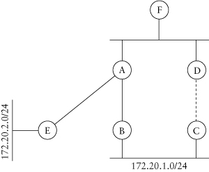
the path to 172.20.2.0/24 through router D instead of the 172.20.0.0/16 received from router A, even though A is a smaller metric! When you scale this scenario to hundreds of remotes attached to a single distribution-layer router, it can cause real problems; a single link failing to a single remote can force all the traffic destined to all the remotes attached to the same distribution-layer router through the dial backup link.
The obvious solution is to summarize on router D, right? Not exactly. Now router E will have two paths to the 172.20.0.0/16 network and will either always choose the path through router A, even though 172.20.1.0/24 is no longer reachable that way, or will load share between the paths through routers A and D.
Not summarizing doesn’t work, and summarizing doesn’t work. What’s left? You can build a distribution list on router C, allowing it to advertise only the 172.20.1.0/24 network to router D. With no summarization, only traffic destined to this one network will pass through the dialup link, leaving us with one other problem, though: How do we get the link to stop passing traffic altogether?
As long as the dial link is operational, router E will see the path through router D as the best way to reach the 172.20.1.0/24 network. It doesn’t matter what the metrics are in this case, because the route advertised by router D is more specific (24-bit prefix length) than the route advertised by router A (16-bit prefix length). Generally speaking, this issue can’t be resolved using an EIGRP solution. Instead, you will need to configure the dial link to be brought down if traffic is flowing in only one direction (interesting traffic) or if the serial interface on router B is up.
In its simplest form, an EIGRP network would contain nothing but native, internal EIGRP routes. In the real world, however, an all-EIGRP network is rare. For various reasons, most networks contain multiple routing protocols, from a few simple static routes to multiple routing protocols with mutual redistribution at multiple points in the network. Redistribution will always bring complexity to an EIGRP network, but if done correctly, it can be handled with few problems.
EIGRP has many types of redistribution, and the following sections discuss the operation and complexity of a couple of them, including redistribution with IGRP (same autonomous system) and EIGRP (different autonomous system). Each section describes the normal operation and expected behavior, along with problems to watch out for and actions to take to decrease the possible problems. But first, we’ll have a brief discussion on redistribution in general.
Redistribution is required when routes learned through one routing protocol must be propagated through another routing protocol. Following are some of the reasons redistribution between protocols might be required:
• Transitioning from one routing protocol to another
• A mix of devices supporting various routing protocols on the network
• The merger of companies using different routing protocols
• Bad network design
Route redistribution in a network is of four general forms:
• One-way redistribution
• Mutual redistribution at one point in the network
• Mutual redistribution at multiple points between two networks
• Mutual redistribution between multiple networks at multiple places
Before reviewing each of these forms of route redistribution and describing the unique challenges each brings to the network design, we need to discuss a complication brought about by performing redistribution between EIGRP and routing protocols that are not capable of supporting routes with variable-length subnet masks.
As discussed in Chapter 1, EIGRP is capable of distributing routes with VLSM (variable-length subnet masks) because it includes the subnet mask for each route in the updates that it sends to its neighbors. Problems can arise, however, when VLSM-based EIGRP routes are redistributed into a routing protocol that is not capable of supporting VLSM networks, such as RIPv1 or IGRP. In the following discussion, we will use IGRP in our examples, but the same complications also hold true for RIPv1.
In Figure 3.20, both the EIGRP and the IGRP portions of the network contain subnets of network 10.0.0.0/8, and EIGRP uses a number of masks for its subnets of that network (/24 and /26 masks). IGRP, on the other hand, cannot handle different masks and thus uses only /24 masks. When router A tries to redistribute the /26 routes into IGRP, IGRP will be unable to propagate them to its neighbors. Why is EIGRP able to handle the different masks and IGRP unable to?
The problem lies in the fact that IGRP (and RIPv1) do not include the mask associated with each route in update packets. Therefore, IGRP has no way to communicate which mask should be associated with each of the routes it is sending to its neighbors. Because of the lack of explicit information, IGRP (and RIPv1) assume that each route in an update packet belongs to either
• The same major network as one or more interfaces on this router—assumes that it has the same subnet mask as the router for that major network
Figure 3.20. Redistribution between IGRP and EIGRP

• A major network that isn’t on any interface of this router—the route uses the classful mask associated with the major network
Therefore, any of the redistributed routes in our sample network in Figure 3.20 with the /26 mask will be discarded by the IGRP process in router A.
One possible solution to this problem is to create a static route on router A to “summarize” the /26 routes from EIGRP into a route that matches the /24 mask used in the IGRP part of the network. For example, router A could contain the static route ip route 10.1.5.0 255.255.255.0 null0 and redistribute it into IGRP. Router A would give the IGRP routers the /24 route they can use and propagate. When a packet is destined to a host on the 10.1.5.64 subnet, IGRP would use the /24 route to get the packet to router A. Router A, in turn, would have the EIGRP routes for 10.1.5.64/26 and 10.1.5.128/26, so it could complete the delivery of the packets to the correct destinations.
Another possible solution is to use a default-network strategy in IGRP, so any target route not contained in the IGRP routing updates will be sent to the default network, which would be the routers doing redistribution from EIGRP to IGRP. All routers in the IGRP part of the network must be using “ip classless” in order for this strategy to work. Unfortunately, if a “true” default network exists in the IGRP part of the network, such as a link to the Internet, this alternative will not work. IGRP would be unable to identify which targets should be sent to the IGRP/EIGRP redistribution point and which should be sent to the Internet access point.
If the non-VLSM part of the network is RIPv1 instead of IGRP, a solution would be to convert it to RIPv2, which supports variable-length subnet masks. Another alternative would be to send a default route (0.0.0.0/0) from the redistributing router into the RIP portion of the network. Similar to the default-network option described for IGRP, this alternative would allow the RIPv1 routers to send all packets destined for target subnets not contained in the routing table to the redistributing router. The same requirement for “ip classless” and the same limitation if there is a “true” default location hold true for the default route strategy in RIPv1.
One more point on this subject. The preceding limitation exists only if the same major network exists in both the EIGRP part and the non-VLSM part of the network. If you are using VLSM in the EIGRP part of the network and are redistributing only the major network into a non-VLSM-capable protocol, this problem doesn’t exist. Only the major network should be sent across the redistribution point, so the non-VLSM protocol should be able to handle it just fine.
Now that we’ve discussed a general problem with redistribution owing to the different capabilities in different routing protocols, we will discuss specific forms of redistribution and the complications each one brings.
One-Way Redistribution: Often, a network will contain devices that must receive routes in a routing protocol other than EIGRP but that don’t need to supply any routes back into EIGRP. A typical example of this scenario is UNIX workstations running routed in quiet mode in order to receive and make local decisions based on routes learned through RIP. In this case, the core of the network may be EIGRP, and the EIGRP routes may be redistributed into RIP at the edges in order to provide routes to the UNIX workstations.
Another example of one-way redistribution is static routes redistributed into an EIGRP network. You may not consider static routes a routing protocol, but when planning for redistribution and filtering, you must consider them as a source of external routes into EIGRP.
ODR can also be redistributed into EIGRP to propagate routes originated at remote sites. Default routing would be used on the remotes to deliver packets into the hub of the network, so EIGRP routes do not need to be redistributed into ODR. In reality, routes cannot be redistributed into ODR at all, so like redistributed static routes, ODR by definition means that there is one-way redistribution.
In one-way redistribution, there is seldom any concern for routing loops or network instability created by a mistaken view of the network. This is by far the safest form of redistribution in a network.
Mutual Redistribution at a Single Point: The second form of route redistribution is mutual redistribution at one point in the network. Figure 3.21 shows an RIP network connected to an EIGRP network, with one router
Figure 3.21. Mutual redistribution at a single point
doing the redistribution. RIP routes are redistributed into EIGRP, and EIGRP routes are redistributed into RIP. With the exception of the problems introduced by connecting a classful routing protocol to a classless routing protocol, mutual redistribution at one point in the network is relatively safe.
You should put filters in place so that routes originating in the RIP domain cannot be relearned inbound in the EIGRP domain, and viceversa, but the filters are probably unnecessary. The route-redistribution process will normally successfully make the right decisions about where routes should point, and instability should not be a major problem.
Mutual Redistribution at Multiple Points between Two Networks: This is where it becomes more of a challenge to make sure that routing instability isn’t caused by the loss of information arising from redistribution. For example, because RIP’s metric (hop count) has no direct relationship to EIGRP’s metric, a somewhat arbitrary metric needs to be artificially applied when routes are redistributed between these protocols. Therefore, the true topological distance required to reach a target network will be lost in the redistribution process, causing the possibility of suboptimal routing or routing loops.
Additionally, when a route is redistributed from one protocol into another at multiple points, the same route may be received on a router from multiple sources from multiple protocols. The router must sort out what the right thing to do is. Combined with the loss of metric information and the various convergence characteristics of various routing protocols, a routing loop or other problems are almost certain.
The most obvious way to prevent problems with mutual redistribution at multiple points is to use distribute-lists between the routing protocols to prevent feeding routes through multiple redistributions. You can also tag the routes, using an EIGRP administrative tag to stop half of this type of routing loop by preventing EIGRP from redistributing external routes back into their original protocol.
Mutual Redistribution between Multiple Networks at Multiple Points: Figure 3.22 shows multiple parts of the network running one routing protocol (IGRP in this case), all connecting at multiple places to a single area of the network running EIGRP. This scenario is a variation of mutual redistribution at multiple points, with the added complexity that many routes will be coming into EIGRP as external routes, will get redistributed into another routing protocol, and will then be relearned from another entry point into EIGRP as a different external route. This can bring disaster! Filtering is absolutely necessary in this scenario in order to increase the odds of stability.
One of the ways in which Cisco IOS increases stability and decreases the likelihood of routing loops is through the use of administrative distances (ADs) assigned to each protocol. The term distance is a bit of a misnomer, as it seems to imply how far something is; in fact, the AD has nothing to do with the metric or path selection within a protocol. Instead, AD refers to the believability of a route learned via a particular protocol. The lower the AD, the more believable the route.
Figure 3.22. Mutual redistribution between multiple networks at multiple points
Table 3.2 shows the relative ADs for IP routing protocols. As you would expect, directly connected routes are the most believable—they exist on this router!—with static routes being the next most believable. Cisco IOS assumes that routes configured by hand should be considered believable!
The AD is used when installing routes in the routing table to decide which one of several matching routes will be installed. For instance, if RIP and EIGRP both attempt to install a route to 10.1.1.0/24, assuming that the EIGRP route is internal, the EIGRP route will be installed. If, however, RIP attempted to install a route to 10.1.1.0/24 and EIGRP attempted to install a route to 10.1.0.0/16, both routes would be installed successfully, because they are not the same route.
The AD is a deciding factor only when both the prefix and the prefix length match. When redistributing between protocols, it’s important to understand how the AD will influence the routes chosen by the router when it’s presented with two paths to the same destination.
Table 3.2. Administrative Distances
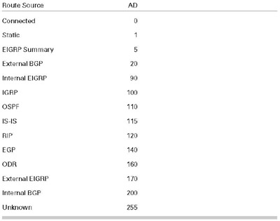
Two commands can be issued in Cisco IOS to modify the administrative distance of routes received from certain neighbors or via certain protocols. For most protocols other than EIGRP, the distance of routes received via a particular protocol can be changed with the following command:
router rip
distance <distance> [address|access-list]
Because EIGRP uses two administrative distances for routes, the syntax of the command is slightly different. Internal and external routes may have their administrative distances set individually. With EIGRP, unfortunately, you cannot limit which routes get this change based on neighbor or access list, as you can in the preceding example. The EIGRP form of the command is
router eigrp 1
distance eigrp <internal> <external>
A word of caution is in order at this point: Be very careful when you decide to change the default administrative distances. Make very sure that you understand the ramifications of the changes, and verify through thorough testing that the behavior will be what you expect.
One additional comment on redistribution needs to be stated. As described in Chapter 2, all redistribution is performed from the routing table. This very important concept is often the source of confusion when routes are not filtered or redistributed in the manner you might expect. For example, if you receive a route to 10.1.1.0/24 via both RIP and OSPF and then redistribute RIP into EIGRP, 10.1.1.0/24 will not be propagated into EIGRP. The path through OSPF will win the AD test (110 for OSPF and 120 for RIP), so the path through RIP will not be installed in the routing table. As it goes to redistribute RIP-derived routes into its topology table, EIGRP looks in the routing table, doesn’t find 10.1.1.0/24 as a RIP route, and thus doesn’t redistribute it.
Similarly, you cannot tell a routing protocol to limit the routes it is redistributing into another protocol. In other words, you cannot tell EIGRP to not redistribute certain routes into OSPF. Again, all redistribution is done from the routing table and is done by the outbound routing protocol. If you want to influence which routes from EIGRP are redistributed into OSPF, you must tell OSPF about it. Redistribution filters can be applied only as a routing protocol is pulling routes out of the routing table.
This behavior is important to understand when deciding how to redistribute and filter redistributed routes. More on this aspect of redistribution will be covered later. Now that we’ve discussed some general redistribution issues, let’s move on to specific cases and how each one behaves.
IGRP in the Same Autonomous System: In almost every case of redistribution, you must manually configure EIGRP to redistribute routes learned from other routing protocols. The only exception when you redistribute between EIGRP and IGRP is if they belong to the same autonomous system. In this case, redistribution is automatic and can be disabled only via the commands
router eigrp <autonomous system>
no redistribute igrp <autonomous system>
When routes are taken from IGRP, the metric is scaled by 256, as EIGRP uses a 32-bit number to represent the metric and IGRP uses a 16-bit number. When it is moved into EIGRP, the IGRP route is identified as an external route with an administrative distance of 170. In the external data section of the EIGRP topology table entry, the advertising router—the router that redistributed the IGRP route into EIGRP—is identified as well as the original IGRP metric of the route.
One additional unique property of IGRP/EIGRP redistribution within the same autonomous system is the interesting case when the administrative distance of the routes is ignored. Here is the one exception to the AD rule! If a route is learned through EIGRP as an external (AD of 170) and IGRP (AD of 100), within the same autonomous system number, the AD is ignored, and the metric, after scaling between IGRP and EIGRP, alone is used to determine the preferred path.
This exception to administrative distance was implemented in order to avoid routing loops while transitioning from IGRP to EIGRP. For example, in Figure 3.23, several clouds of IGRP networks are connected
Figure 3.23. Administrative distance in IGRP-to-EIGRP redistribution
to a core of EIGRP. This situation may be short-lived during a transition from IGRP to EIGRP, or it could remain for a period of time. Let’s look at what would happen if the exception to the administrative distance rules didn’t exist.
As the route to 10.1.1.0/24 is redistributed into EIGRP by router C from the IGRP cloud on the right, the route goes from having an administrative distance of 100 for IGRP to 170 for an EIGRP external. As it passes through the EIGRP cloud and is redistributed into the IGRP cloud on the left by router A, the route becomes an IGRP route again, which doesn’t have any concept of an external route, and thus has an administrative distance of 100.
Router B will now have two routes to 10.1.1.0/24—one through IGRP as it was redistributed by router A and an EIGRP external as it was redistributed by router C. Which route should router B choose? According to normal processing using the administrative distances of the two routes, the IGRP route would be preferred! This is obviously incorrect.
Instead, the behavior was changed so that router C, when it receives the same route as an EIGRP external and through IGRP, compares the metric—with the IGRP metric scaled by 256—in order to determine which path is the most direct to the target network. In this case, the EIGRP external route to 10.1.1.0/24 would be preferred and would be installed in router C’s routing table, even though it has a higher administrative distance than the IGRP route.
With this somewhat nonintuitive behavior, redistribution between IGRP and EIGRP in the same autonomous system is fairly safe and normally will provide the desired functionality. This built-in safeguard will keep poor next-hop selections from being made and will normally create a stable network. The following section describes a much different picture.
Multiple EIGRP Autonomous Systems: It’s fairly common to see large EIGRP networks divided into a number of separate EIGRP autonomous systems with mutual redistribution between them. This may be done for three reasons:
• Defining the scope of administrative control, with each autonomous system controlled by a different group of people
• Merging companies
• Attempting to reduce query range
In the first and second cases, the reason chosen for multiple autonomous systems is more of a political or a management decision, not a technical decision. In reality, if multiple EIGRP autonomous systems are used with mutual redistribution between them, very little in the way of protection or autonomy is provided. Unless other techniques, such as summarization or distribution lists, are used, a link flap in one AS will be felt in the other autonomous systems as well. If summarization or route filtering is used to stop this propagation from happening, the information hiding through summarization/filtering—not the multiple autonomous systems—is making the network more robust.
The third reason is probably the most common one for choosing to implement multiple EIGRP autonomous systems. During the early days of EIGRP, network instability owing to SIA routes was extremely common, and not many tools were available to stop the problems. By defining multiple EIGRP autonomous systems, the timing of the SIA process is indeed changed a little, and a minor increase in network stability could be the result. Unfortunately, the complexity of route redistribution and the routing loops caused by the redistribution are far more harmful than the benefits gained.
First, the benefits of multiple autonomous systems will be explained. Figure 3.24 shows a network comprising multiple EIGRP autonomous systems with mutual redistribution between them. When the route to 172.20.40.0/24 on the left goes active owing to a link flap, queries flow throughout AS 1, looking for an alternative path to reach this network.
Figure 3.24. Mutual redistribution between multiple EIGRP ASs
When the query reaches router B, it replies to the original query but then starts another one of its own in AS 2. When this query reaches the router C, the second query process is terminated via a reply, but a new query process is started in AS 3!
The timing of the query process has been changed. Instead of router A waiting for a reply until router D has finished processing the query, router A receives a reply when router B processes the query. A second and then a third query process are started independently, and each must be terminated in order to successfully converge on the topology change. At least the router that originally asked the question will not get an SIA due to a link problem in the third AS!
The good news is that the router that originated the query won’t generate an SIA. The bad news is that redistribution between multiple EIGRP autonomous systems creates very significant complexities and can cause much harm. Let’s take a fairly simple example. In Figure 3.25, we again have multiple EIGRP autonomous systems connected via multiple points of entry, as well as a cloud of RIP routers in our network. When the route to network 172.20.40.0/24 is originated in RIP, the route has an AD of 120 throughout the RIP domain. When it is redistributed into EIGRP AS 1 by router B, the route becomes an external route and thus has an AD of 170 throughout AS 1. The route is then advertised into AS 2 by router C, where it continues to have an AD of 170. Here’s where it gets interesting.
Thanks to the redistribution in router C, the route to 172.20.40.0/24 will be learned on router D from two directions: as an external route via AS 1 and as an external route via AS 2. So which path will win on router D: the one through AS 1 or the one through AS 2? Logic says that the
Figure 3.25. Multiple EIGRP autonomous systems
path through AS 1 will win because it is obviously a shorter path: It has a smaller metric through AS 1 than through AS 2.
Unfortunately, this isn’t how it works. Routing protocols use the metric to select a path between alternative paths within a single instance of a routing protocol. If the same route—prefix and prefix length—is learned via two routing protocols, the metric is ignored! The exception, as described earlier, is for routes learned via EIGRP (external) and IGRP in the same autonomous system. Other than this exception, the metric plays no part in path selection when comparing routes learned via different routing protocols, including multiple EIGRP autonomous systems! So how is the path selection made?
The path selection criterion, as described earlier, is the administrative distance. The path learned via the routing protocol with the lowest AD will be the one put into the routing table. But wait! In our example, the path to 172.20.40.0/24 is learned on router D from both EIGRP AS 1 and EIGRP AS 2 as externals, so both routes have an AD of 170. Which one wins? Unfortunately, the result will not be consistent: Whichever route is installed in the routing table first will win.
How can you avoid this problem? Careful route filtering at the redistribution points is required to keep these feedback loops from creating havoc in your network. The next section discusses the most common method of performing route filtering at these redistribution points: distribution lists.
Route Filtering: Earlier, route filtering was described as a method of hiding information in order to decrease query scope and complexity in the network. Route filtering can also be used to eliminate the propagation, or acceptance, of routes that would create routing loops or suboptimal routing in a network. For example, route filters are commonly used at redistribution points in order to make certain there won’t be routing loops owing to AD problems. This use is crucial when there are multiple points of redistribution between multiple routing protocols.
An example of the damage that can be caused is depicted in Figure 3.26, which shows the route to 172.20.40.0/24 entering EIGRP as an external and flowing through AS 1, having an AD of 170 on each EIGRP router. As the route is redistributed from EIGRP AS 1 into AS 2, it continues to have an AD value of 170. The problems begin when the route is redistributed by router C into AS 2; router D receives two EIGRP external routes, both with an AD of 170, and must choose between the two. Which one gets installed? The answer is indeterminate: There is no way of knowing which one will be installed. The one that is installed, however, will be redistributed into the other AS; for example, if router D decides to install the AS 2 route in its routing table, router D will redistribute the AS 2 route back into AS 1.
The only way to make certain the right route is installed is to put a distribution list inbound under AS 2 on the routers redistributing between AS 2 and AS 1, denying the routes that originated in AS 1, originally a RIP route, from being learned inbound from AS 2. This configuration can be administratively troublesome, keeping these access lists correct as network changes occur, but it needs to happen in order to ensure that routing is correct.
Figure 3.26. Route filters to prevent routing loops

We’ve now covered a number of design issues that must be considered when designing an EIGRP network, but a couple of other design questions are often asked by people building networks using EIGRP. These common questions will be discussed in this section.
Probably the most frequently asked question is, How many neighbors are too many for an EIGRP router? Considerable cost savings are possible in having as many remote sites connect to the same distribution router as possible, particularly if the traffic requirements for each remote site are fairly small and regular. Early in the life of EIGRP, Cisco typically recommended no more than 30 neighbors per router, but this limit obviously doesn’t support the density required by networks today.
With proper design, an EIGRP router will reliably support many more than 30 neighbors. How many more can be supported? It depends! It depends on how much information is being sent to the remotes, whether the remotes are stub sites, the speed of the links, the stability of the network, and a myriad other factors. Unfortunately, we cannot state a magic number to use or even a magic formula to apply to determine the maximum allowable neighbors. Instead, we will discuss how each factor influences the maximum number of neighbors so that you can make a reasonable estimate of how many neighbors a router can handle.
The first consideration is how many routes must be exchanged with each remote router. If the remote site has a single link to the remainder of the network, it really doesn’t need any! A default route on the remote router will suffice to send traffic to the distribution router and will need to advertise to the distribution router only whatever routes originate at the remote site.
In Figure 3.27, router A can reach the rest of the network only through the connection between the two routers, so a default route pointing to router B is all that’s necessary for passing traffic into the network from the remote site. Router A would be responsible for sending in the routes located at the remote site so distribution router B can propagate them to the remainder of the network. In this case, very little routing update traffic would be required with any remote site.
Figure 3.27. A simple remote site routing situation
If the remote site requires receiving at least a single route for its dial backup strategy to work properly, the preceding holds true. The distribution router B would send a single default route to router A, and router A would send its local routes to router B. Again, very little routing information would need to be passed to the remotes.
In both of these scenarios, the amount of update traffic to the remotes is very small. Unfortunately, unless the remote routers are defined as stub routers, all these remote routers would still be involved in the query process. Distribution lists and summary statements limiting updates from router B to router A will limit updates to a single default—or even nothing—but that will not stop queries. By defining the remote routers as stub routers, even queries will not be sent to the remote sites.
A third scenario is if the remote site has dual frame relay PVCs and needs at least some routes from each distribution site, as shown in Figure 3.28. This situation may happen if the two frame relay circuits terminate at distribution routers that are geographically dispersed and there is significant delay or congestion to send traffic to the “wrong” distribution router. In this case, more routes must be exchanged with each remote site, increasing the work EIGRP must perform. In this type of network, distribution lists must be put on the remote routes so remotes do not reflect routes learned from one distribution router back to the other distribution router.
The fourth scenario is if the network is not hierarchical and remote sites are connected to one another. These “back-door” links can be fully meshed or partially meshed. In this scenario, far more routing knowledge
Figure 3.28. Dual-homed remotes
is required on the routers in order to select the correct next hop, and the complexity of the query path is dramatically increased. EIGRP’s job can be extremely difficult in this type of network.
Besides the route count and complexity, other factors influencing how many neighbors are allowable include the CPU power of the routers involved, the stability of the network, and the link speeds to reach those remote sites. If links are not stable or are congested or if routers are underpowered, EIGRP will be less likely to respond quickly to topology changes and will more likely be unable to converge successfully.
As the complexity and route requirements increase, you should decrease the number of neighbors. With only default routing and high-powered distribution routers, such as RSP4s or 7200s with NPE300s, we’ve successfully tested in the lab with 500 neighbors! Other networks cannot retain stability with 10–20 neighbors if there are many routes, no hierarchy, route reflection, and unstable links. Using the simplifying techniques described in this chapter, 300 neighbors have been implemented successfully in a production network.