Chapter 1
The diagnostic process
Introduction: epidemiology in the clinic
Common things are common
Patients are drawn from a wider population, and through our knowledge of the distribution of disease in that population we can have an idea of the range of likely diagnoses for our patients. Before taking any history, performing an examination, or ordering investigations, you should have some background knowledge of the frequency of different conditions. This essential underpinning of clinical decision-making, rarely reflected upon, is based on epidemiology. If something is very rare, in everyday practice it will remain lower on your differential diagnosis list than if it is common. How is this distribution of disease described? How common is breast cancer, for example? There are many ways of answering this question, some being more relevant to clinical practice than others. Many people know that one in eight women will suffer from breast cancer at some point. But this does not show the probability that one of your patients has breast cancer at this time. More precise measures are needed, including prevalence and incidence, as outlined on pp.6–8.
Index of suspicion
In addition to knowledge of disease frequency, a diagnosis is based on understanding the distribution of disease according to certain inherent criteria such as age and sex, and according to risk factors or exposures such as smoking or occupation. Again most clinicians will have an appreciation of these factors and they will adjust their differential diagnosis accordingly. Mesothelioma will be high up the differential diagnosis of a patient with pleuritic pain, cough, and weight loss who has a history of occupational exposure to asbestos, for example. Ways of quantifying the relationship of exposures to disease, as measured in epidemiological studies, are described on pp.12–15.
Refining the diagnosis
Quantifying information on the frequency of disease in the population and the impact of different risk factors on that frequency can be used to produce a measure of the likelihood that a person will have a certain condition. This pre-test probability should be the starting point for carrying out examinations and investigations which will then aim to increase, or decrease, that probability according to their results. Each test, whether a simple examination or a complex metabolic or imaging technique, has a likelihood ratio that can be used to increase or decrease the probability of the condition according to the test result. In much clinical practice this process is carried out in a qualitative way—with a result sometimes being considered to rule in or rule out a condition, but in reality few tests carry such certainty. On pp.22–25. we explain how to use results in a quantitative way, producing post-test probabilities of disease.
This section ends with a summary of how information can be put together to reach a diagnosis, and how to communicate this to patients (‘So what have I got, doctor?’). This then forms the starting point for Chapter 2 on the management of patients.
Measures of disease frequency
In order to describe the distribution of a disease there must be an agreed definition of a case (see p.10) and this may vary according to the purpose of the measure.
Count
Definition: the number of cases:
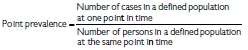
Prevalence
See also p.167.
Definition: the proportion of people with a disease at any point (point prevalence) or period (period prevalence) in time.
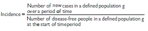
Incidence
See also p.179.
Definition: the number of new cases of the disease in a defined population over a defined period of time. Incidence measures events (a change from a healthy state to a diseased state).
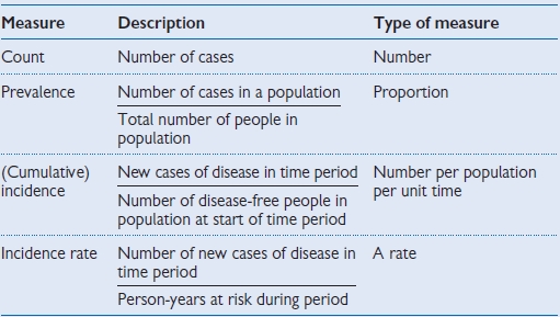
Relationship of incidence and prevalence (Table 1.1)
Table 1.1 Measures at a glance
Examples (Tables 1.2 and 1.3)
Table 1.2 Relationship of incidence and prevalence in breast cancer
| Measure | Breast cancer, women in UK, 20091 |
|---|---|
| Prevalence | 550000 women are alive in UK who have had a diagnosis of breast cancer (2% of adult female population) |
| Incidence | 47700 new cases 124 per 100000 per year (European age-standardized incidence) |
| Lifetime risk | 1 in 8 |
Table 1.3 Relationship of incidence and prevalence in genital chlamydial infection
| Measure | Chlamydia trachomatis in 15–24-year-olds, 20092 |
|---|---|
| Count | 482,696 cases diagnosed in sexual health clinics and community settings in the UK |
| Prevalence | 5–7% in National Chlamydia Screening Programme, England |
| Incidence | 2180 per 100,000 per year in England |
| Lifetime risk | 30–50% for women by age 35 (2005 estimate) |
Understanding prevalence: HIV infection
In the UK, the prevalence of HIV infection is increasing. Interpreting this finding requires an understanding of several factors:
Distribution of disease
Rare things can seem common
As a medical student attached to a paediatric oncology firm it seemed as if all children with a sore throat or with bleeding gums had leukaemia. Clearly the millions of children with self-limiting viral upper respiratory tract infections or gingivitis would not make it into this centre. The distribution of disease seen in clinical practice is not the same as that in the population, and therefore interpretation of signs and symptoms will depend upon where you practise.
Common things are common (but can seem rare)
Just as rare things can seem common, so some common things are rarely seen by some clinicians—the clinical iceberg. It is important to understand the background distribution of disease in the population generally, and also in the population seen in your practice (whether through referral or self-presentation).
Finding out
Finding out how common conditions are in the population is challenging. Most data are based on reported illness, which is severe, or from healthcare settings which necessarily excludes all those conditions that are managed at home. Special population surveys are needed to find out the prevalence of disease, but these tend to focus on symptoms and self-report rather than confirmed diagnoses. In other words, they are measuring different things. The clinical iceberg concept indicates how little illness appears on the radar if health is measured through mortality, hospital data, or even primary care data.
Seeking advice
The 10 most common symptoms of adults seeking advice from NHS Direct in England are abdominal pain, headache, fever, chest pain, back pain, vomiting, breathing difficulties, diarrhoea, urinary symptoms, and dizziness.
Primary care consultations
The most common consultations for adults in primary care are for respiratory illness and neurological conditions.
Secondary care admissions
The most common hospital admissions in England (2009–10 data) are: cardiovascular and respiratory disease and symptoms (15%); gastrointestinal disease and symptoms (15%); and cancer (11%).
Mortality
The leading causes of death in the UK (2005 data) are circulatory disease (36%), neoplasms (27%) and respiratory disease (14%).
Is there anything wrong?
Patients are first concerned with finding out whether they have anything wrong with them, and if so, what it is, can it be cured, what the future holds, and then, often a little later, why them?
Deciding whether there is anything wrong is not always easy, since perceptions and definitions of health and disease vary. The World Health Organization (WHO) definition of health is a state of complete physical, mental, and social well-being and not merely the absence of disease or infirmity. By that definition a large proportion of people are unhealthy.
For the clinician, defining and labelling a patient with (or without) a specific disease is the key to decision-making. However, definitions are rarely clear-cut. While clinical medicine depends on distinguishing normal from diseased states, these are generally rather arbitrary distinctions since there is a range of normality and of disease which frequently overlap. In practice we are looking for a definition or cut-off which divides people into those who would benefit from treatment and those who would not, and of course such definitions may change over time.
Purpose of defining a case
The purpose of defining a case varies by setting:
Labels
For some conditions a diagnosis is a label with wide-ranging implications for the patient in relation to family, finances, employment, etc. Some labels carry a stigma and therefore the clinician must be particularly careful and sensitive before making the diagnosis.
Difficulties in defining a case
Have I got hypertension?
Defining hypertension is important as is it relates to high levels of morbidity and mortality. But blood pressure (BP) has an essentially normal distribution in the population. At the upper end of the distribution are people with severe or ‘malignant’ or accelerated hypertension which is life threatening in the short term. Below this point there is no easy level at which to distinguish ‘hypertensive’ and ‘normotensive’. In general, hypertension is defined at a level that indicates the need for treatment to reduce the risk of coronary heart disease and stroke. But the risks start to increase at a very low level, and therefore it is still somewhat arbitrary to decide that a certain amount of increased risk justifies treatment. Ideally we would define cases as those people in which intervention (e.g. antihypertensive drugs) will be more beneficial than no intervention.
The normal distribution
The frequency of many human characteristics in the population (height, weight, blood pressure, haemoglobin, serum albumin etc.) tends to follow a normal distribution or bell curve. For many diagnostic tests of continuously distributed variables, ‘normal’ is defined statistically as lying within 2 standard deviations of the mean of the distribution of variation among individuals (see p.230). This mathematical method of defining normality is rather arbitrary and may or may not relate to disease processes.
Risk factors
Disease is not evenly distributed across the population, and epidemiology is concerned with exploring the factors associated with that variation. Understanding the major determinants of health and disease helps clinicians in drawing up a differential diagnosis for a particular patient. For example, you are more likely to consider infective endocarditis as a diagnosis if a person presenting with fever has a prosthetic heart valve. Similarly, the possibility of bronchial carcinoma will be higher up the differential diagnosis in a smoker with haemoptysis than in a non-smoker, and Weil’s disease will be more likely in a farm worker than a computer programmer if both present with headache and fever followed by jaundice. Thus understanding and quantifying risk factors can assist in the diagnostic process as well as informing preventive interventions.
Definitions
Relevance to clinical practice
Quantifying risk factors
Epidemiological research is largely concerned with exploring the relationship between risk factors (exposures) and disease (outcomes). The following parameters describe the association:
Chapter 7 includes detailed definitions and methods for measuring these parameters (see pp.145–195). In clinical practice it is useful to remember what each of them means for patients:
The relative risk (pp.179–180) tells you how much more likely a disease will be in a person with a risk factor than a person without it. It is estimated in cohort or follow-up studies from the incidence in the exposed (those with the risk factor) divided by the incidence in the unexposed, i.e. Ie/Io. Using the example in Box 1.1, a woman on hormone replacement therapy (HRT) is 2.25 times more likely to develop breast cancer than a woman who has never taken HRT.
The attributable risk (pp.179–180) tells you the absolute increase in incidence of disease that is associated with the risk factor, and is also estimated from cohort studies from Ie− Io. Again, the data in Box 1.1 would suggest that the woman taking HRT has an extra risk of 2.1 cases of breast cancer per 100 women years which is equivalent to an extra 2.1% chance of developing breast cancer each year as a result of the HRT (assuming a causal relationship).
The odds ratio (pp.172–174) is an estimate of relative risk obtained from case–control studies where the incidence of disease is not known, but the frequency of exposure is measured in cases and controls. Its use with patients is the same as relative risk.
Correlation (pp.162, 262) is another measure of association that is used for risk factors that are continuous variables or multiple categories. A correlation coefficient (r2) shows how much an increase in risk is explained by an increase in exposure.
Box 1.1 Quantifying risk factors: example of breast cancer and HRT1
Danish women were enrolled in a cohort study, and the relationship of HRT to breast cancer incidence was explored.
The incidence of breast cancer was 1.68 per 100 women per year for those who had never used HRT, and 3.78 for those currently on HRT.
Relative risk = incidence in exposed (Ie)/incidence in unexposed (Io)
= Ie/Io
= 3.78/1.68
= 2.25
Attributable risk = incidence in exposed − incidence in unexposed
= Ie − Io
= 3.78 − 1.68
= 2.1 per 100 women per year
Identifying risk factors
In the consultation obtaining accurate information on relevant risk factors can help in forming a differential diagnosis. This is usually done by taking a structured history that should include demographic, occupational, social, and behavioural factors.
Taking a risk factor history
Questions must be:
To obtain accurate risk factor information requires skill in communication. The patient will need to understand why certain questions are being asked, and feel confident that the information is pertinent, confidential, and will not be used in any prejudicial way.
Reliable histories
Some risk factor questions are notoriously difficult to collect reliable information on. This may be due to sensitivities (see Box 1.2) or real difficulties of recall. Where possible, previous records should be consulted for exposures such as vaccinations, previous drug treatments, occupational history and possibly lifestyle (if these are routinely collected).
Box 1.2 Sensitive questions
Country of origin, nationality, ethnicity
Sexual behaviour, sexuality
Drug, alcohol, and tobacco use
Other lifestyle factors
Reassurance
Improved information on sensitive issues may be obtained if:
Validity of diagnostic tests
When we order a diagnostic test, or carry out a particular examination, the intension is to make a definitive diagnosis or at least narrow the differential. Unfortunately, few if any tests are 100% correct 100% of the time.
Far from being a definitive answer, most tests require some interpretation. The key parameters for describing the validity of a test are its sensitivity and specificity. Interpreting the results of tests requires an understanding of how they perform (Tables 1.4,1.5, 1.6).
Definitions
Parameters of validity
These parameters are also incorporated into the concept of likelihood ratios which are particularly useful in clinical practice as they can be used with pre-test probabilities in quantitative diagnostic analyses (see Likelihood ratios, p.22).
Helpful reminders
Table 1.4 Calculating the parameters of a diagnostic test
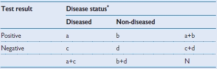
* According to gold standard
• Sensitivity: a/(a+c)
• Specificity: d/(b+d)
• Positive predictive value: a/(a+b)
• Negative predictive value: d/(c+d)
Table 1.5 Alternative representation
| Test result | Disease status* | ||
|---|---|---|---|
| Diseased | Non-diseased | ||
| Positive | True positive | False positive | |
| Negative | False negative | True negative | |
* According to gold standard
• Sensitivity: true positive/(true positive + false negative)
• Specificity: true negative/(true negative + false positive)
• Positive predictive value: true positive/(true positive + false positive)
• Negative predictive value: true negative/(true negative + false negative)
Table 1.6 Worked example of test performance for a rapid test for genital Chlamydia infection
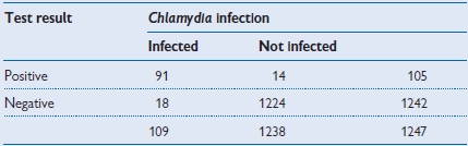
| • Sensitivity: | 91/109 = 83.5% |
| • Specificity: | 1224/1238 = 98.9% |
| • Positive predictive value: | 91/105 = 86.7% |
| • Negative predictive value: | 1224/1242 = 98.6% |
Reference
1 Mahilum-Tapay L et al. New point of care Chlamydia Rapid Test—bridging the gap between diagnosis and treatment: performance evaluation study. BMJ 2007; 335:1190–4.
Clinical uses of predictive value
The predictive value of a symptom, sign, or test is a very useful parameter in clinical practice. It is a measure of how likely the patient is to have (or not have) a condition given that they have had a positive (or negative) result.
These values enable you to answer that common question from a patient: ‘You tell me the test is positive (or negative), so have I definitely got (or not got) the disease?’
Pathognomonic?
For some conditions, a positive sign or test is said to be a definitive answer or pathognomonic. This can only happen when the test is completely specific, i.e. there are never any false positives, and therefore the PPV is 100%. There are probably no truly pathognomonic signs, but they were traditionally said to include rice-water stools (cholera), risus sardonicus (tetanus), Koplic’s spots (measles). For a symptom, sign, or test to be fully diagnostic, then all people with the disease are positive and all those without are negative. The PPV and NPV would both be 100%, and the test would be the gold standard and a way of defining the condition. However, for the majority of conditions such simple certainty is not present, at least with preliminary tests, and we are left with interpreting differing levels of certainty.
Predictive value varies
Unlike sensitivity and specificity, predictive value is not based only on inherent test characteristics, but varies according to the prevalence of the disease in the population as well as the sensitivity and specificity of the test. This is best understood using a worked example (see Tables 1.7–1.9).
Practical use of predictive value
When a patient has had a test and the result is available, they will usually expect a definitive answer. In a number of situations you will need to discuss the uncertainty of test results in a meaningful way. Telling patients that the test has a good sensitivity or specificity is not particularly helpful as they have no way of relating that information to their own situation. Predictive value can be more useful on the proviso that it relates to a population with a similar prevalence to that of the patient in front of you.
Using the data in Tables 1.7,1.8, 1.9, if you carried out a such a HIV test in apatient attending a similar primary care setting and the result was positive, you could explain to the patient that a positive test is only truly positive half of the time, and therefore they need to wait for a confirmatory test. On the other hand, if their result is negative, you could confidently say that they were free from the disease (assuming there had been sufficient time since the presumed exposure).
In the next sections (see pp.20–25) we show how knowledge about prevalence and test validity can by systematically incorporated through use of pre-test probabilities and likelihood ratios.
Predictive value varies with prevalence: worked example
Imagine that there was a new rapid test for HIV infection, and it had a sensitivity of 100% and a specificity of 99%. That means that everyone with HIV will test positive, but for every 100 people without HIV, 1 would also test positive. Tables 1.7–1.9 show the results of using the test in 3 different populations.
In these 3 different populations a test with the same sensitivity and specificity produces widely different PPV. If it were used for screening a low-prevalence population there would be a lot of false positives that would need to be subject to a confirmatory test.
Table 1.7 Test used in a sexual health clinic with a high prevalence population (prevalence = 10%)
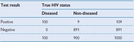
• Positive predictive value = 100/109 = 91.7%.
Table 1.8 Test used in a primary care setting (prevalence = 1%)
• Positive predictive value = 10/20 = 50%.
Table 1.9 Test used in a blood donor population (prevalence = 0.1%)
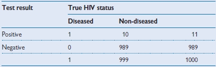
• Positive predictive value = 1/11 = 9.1%.
Pre-test probability
The process described up to now—moving towards a diagnosis based on knowledge of the distribution of disease in the population and risk factors, together with the basic history of the patient—provides a starting point for the ordering of specific investigations or tests. A test may be as simple as a physical examination or as complex as the latest imaging techniques but should be undertaken with the same purpose: to move closer to, or further from, a given diagnosis.
Definition of pre-test probability
The probability of the condition or disorder before a diagnostic test result is known.
The pre-test probability is the likelihood that the patient has the condition when you do not know the result of the test. At its broadest, this is the prevalence of the condition in the population, but in practice it should be related to the specific patient as far as possible and include the clinical setting, the age, sex, with or without known risk factors, and presenting with a particular set of symptoms or signs. In general this is unknown, and we work with a more qualitative approach based on past experience of similar patients and knowledge of risk factors, but with the growth of evidence-based clinical practice tools to quantify such information are likely to be made available.
There are a number of conditions where pre-test probabilities are well described (see Box 1.3) and these may be useful in clinical decision-making. In practice few clinicians have the time to carry out formal calculations of pre-test probabilities before deciding on investigations, but such quantitative analyses are increasingly used to inform clinical decision support tools such as algorithms and guidelines (see p.38).
Box 1.3 Pre-test probabilities1
Syncope
Setting: community hospitals in Italy.
Findings: of 195 patients with syncope, 35% (69) had neurovascular reflex disorders, 21% had cardiac disorders. Particular factors in the history shifted the probabilities; e.g. a lack of cardiac findings on examination and electrocardiogram (ECG) lowered the probability of cardiac disorders for this patient.
Use: such information can help in reaching diagnosis by providing a hierarchy of possibilities from the 50 or more reported causes of syncope. Investigations or, if appropriate, a trial of a treatment can then be directed to try and confirm or exclude the most likely diagnosis or diagnoses.
Chest pain2
A 65-year-old man comes in to see his general practitioner (GP) with chest pain
Objective of diagnostic process
Pain caused by myocardial ischaemia in impending infarction must be differentiated from non-ischaemic chest pain in order to inform management of the patient.
How do you tell if this is likely to be cardiac chest pain?
You could list all the causes of chest pain and systematically test for each one, but it is far more efficient to start by narrowing it down based on what you already know.
What do we know now?
From this information you can calculate a pre-test probability that he has CHD. This can be done qualitatively, based on ‘experience’ and prior knowledge, or can be done quantitatively using precise estimates based on epidemiological data. Using such a method, the authors of this example estimated a probability of 25% that this man had severe CHD (see website2 for details and tutorial).
Likelihood ratios and post-test probabilities
Likelihood ratios are a useful way of quantifying results in the diagnostic process by relating the probability (p) of a result in someone with the disease to someone without it. The likelihood ratio (LR) is the likelihood that a given test result would be expected in a patient with the disease compared to the likelihood that that same result would be expected in a patient without the disease.
Their usefulness over and above other measures of validity is that they can be applied to a pre-test probability to produce a numeric increase or decrease in that probability given a particular test result. A LR >1 is associated with the presence of the disease, and the higher the number the stronger the association. A LR <1 is associated with the absence of the disease, with the lower the number the stronger the evidence for absence (Table 1.10).
Positive likelihood ratio (LR+) is a measure of how much to increase the probability of disease if the test result is positive:
Negative likelihood ratio (LR−) is a measure of how much to decrease the probability of disease if the test result is negative:
Table 1.10 Estimated likelihood ratios for diagnosing urinary tract infection (UTI) from symptoms in previously healthy women
| Symptoms | +LR | −LR |
|---|---|---|
| Dysuria | 1.5 | 0.5 |
| Frequency | 1.8 | 0.6 |
| Haematuria | 2.0 | 0.9 |
| Back pain | 1.6 | 0.8 |
| Vaginal discharge (absence) | 3.1 | 0.3 |
| Vaginal irritation (absence) | 2.7 | 0.2 |
| Low abdominal pain | 1.1 | 0.9 |
| Flank pain | 1.1 | 0.9 |
| Self-diagnosis | 4.0 | 0.1 |
| Symptom combination of +dysuria, +frequency, −discharge, −irritation | 24.6 | (n/a) |
Estimating post-test probabilities using likelihood ratios
The calculation is done using odds rather than probabilities which can be a bit complicated and slow (see Box 1.4). In practice there are short-cuts using calculators (available online:  http://www.cebm.net/index.aspx?o=1161) or a nomogram (see p.24). To do the calculations by hand you need to be able to convert probabilities (p) to odds (o) and vice versa using the following general formula:
p = o/(1 + o)
Then pre-test odds are:
and the post-test odds, in a person with a positive test are:
which can be converted back into a probability to help communicate the risk to the patient:
where o1 is pre-test odds, o2 is post-test odds, p1 is pre-test probability and p2 is post-test probability.
These estimates of LR are made from a systematic review of evidence applied to women presenting with possible UTI with a pre-test probability of 50%. The author concludes, ‘Combinations of symptoms . . . may rule in the disease; however, no combination decreases the disease prevalence to less than 20% . . .’.1
Box 1.4 Example of calculating post-test probabilities
What is the role of a dipstick test in the diagnosis of UTI in symptomatic women attending GPs? The prevalence of UTI in symptomatic women (pre-test probability) was 55%, the dipstick sensitivity 90%, specificity 65%.
For a positive test:
LR+ = sensitivity/(1 − specificity) = 0.9/(1 − 0.65) = 2.57
p1 (from prevalence) = 0.55
o1 = 0.55/(1 − 0.55) = 1.22
o2 = o1 × LR+ = 1.22 × 2.57 = 3.14
p2 = 3.14/(1 + 3.14) = 0.76
For a negative test:
LR− = (1 − sensitivity)/specificity = (1 − 0.9)/0.65 = 0.15
o2 = o1 × LR− = 1.22 × 0.15 = 0.18
p2 = 0.18 /(1 + 0.18) = 0.15
Conclusion
In a woman presenting in general practice with symptoms suggesting a UTI, a positive dipstick test increases the probability of a bacterial UTI from 55% to 76%, while a negative dipstick test decreases the probability to 15%.
Fagan nomogram
The Fagan nomogram allows LR to convert pre- to post-test probabilities. To use, if the pre-test probability is marked on the left axis, then a line is drawn from this point on the left side of the graph through the LR value (positive or negative) for the test. The point where the line meets the right side of the graph is the estimated post-test probability of the disease (Fig. 1.1).
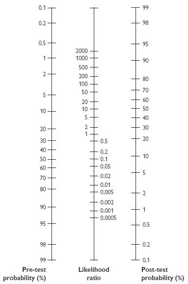
Fig. 1.1 Fagan nomogram. Reproduced with permission from Greenhalgh T. How to read a paper: Papers that report diagnostic or screening tests. BMJ 1997; 315:540–3.
Online resource
Links to a number of likelihood ratios can be found at Bandolier. http://www.medicine.ox.ac.uk/bandolier
So what has my patient got? The Bayesian clinician
The processes described in the previous sections of this chapter are all about narrowing the differential diagnosis through gathering together evidence. This is inherent in diagnostic decision-making, although we rarely think of it in these terms. The process is akin to Bayesian statistics, and if quantified through pre- and post-test probabilities and LRs it is an actual application of Bayes’ theorem. Bayes’ theorem states that the pre-test odds of a hypothesis being true multiplied by the weight of new evidence (LR) generates post-test odds of the hypothesis being true. Unlike ‘frequentist’ approaches to statistical inference, Bayesian inferences explicitly include prior knowledge, in these examples the pre-test probability. At each step in the diagnostic process you have a working idea of the probability of a diagnosis, and with the results of each question, examination and investigation you increase or decrease that probability.
In routine clinical practice this process is usually more qualitative than quantitative due to lack of relevant LR estimates, lack of time, and lack of expertise. However, quantitative estimations are important in developing clinical decision-making tools and algorithms to guide clinicians and increasingly to direct nursing and other healthcare staff in face-to-face, telephone, or online consultations. They can also be applied in clinical governance to reduce unnecessary investigations or introduce new ones.
Increasingly, new technologies are being used to improve clinical decision-making.
Clinical scoring systems
There are a large number of clinical scoring systems to assist diagnosis. Like any tool, some are better than others, and can be evaluated in terms of sensitivity and specificity.