Differential Calculus
Abstract
We could cite various forerunners of differential calculus, including Descartes, Fermat and Cavalieri, but Newton and Leibniz should be remembered as the true pioneers of the field. This dual paternity created terrible priority disputes where the only certainty is the complexity of the controversy. Newton’s “fluxions” and Leibniz’s “vanishing quantities” are analogous to our modern concepts of derivative and differential, respectively. The extension of these ideas to functions of several variables was due to Euler (who introduced partial derivatives) and Clairaut. After contributions by many other mathematicians, including Volterra and Hadamard, the concept of a derivative of arbitrary order (Lemma-Definition 1.4) was ultimately introduced by Fréchet between 1909 and 1925. The inverse mapping theorem was proved by Lagrange in 1770, and the simplest case of the implicit function theorem was proved by Cauchy around 1833, followed by the case of vector-valued functions of several variables by Dini in 1877. Gateaux then extended Fréchet’s earlier ideas to develop his concept of differential, which was presented in a posthumous publication in 1919. The “convenient” form of differentials, one of their most recent incarnations, was introduced by Frölicher, Kriegl and Michor in the early 1980s (p. 73). These differentials were intended for mappings taking values in locally convex non-normable spaces, in particular nuclear Fréchet spaces (see, in particular, section 5.3.2 on manifolds of mappings). Wherever possible, this chapter therefore chooses to present differential calculus for mappings which take values in locally convex spaces rather than the normed vector spaces considered by the standard approach (nothing essential changes). Nonetheless, for the inverse mapping theorem and the implicit function theorem (Theorems 1.29 and 1.30), we will restrict attention to the Banach case (for a more general context, which uses yet another concept of differentiability distinct from any of those mentioned above). Both theorems are proved in full detail, including the Banach analytic case, by explicitly filling in the hints from. Together with the Carathéodory theorems mentioned below, these two theorems are the most profound results of this chapter.
Keywords
Calculus of variations; “Convenient” differentials; Differential Calculus; Existence and uniqueness theorems; Fréchet differential calculus; Gateaux differentials; Lagrange variations; Mappings of class Cp; Parameter dependence; Taylor’s formulas
1.1 Introduction
We could cite various forerunners of differential calculus, including Descartes, Fermat and Cavalieri, but Newton and Leibniz should be remembered as the true pioneers of the field. This dual paternity created terrible priority disputes where the only certainty is the complexity of the controversy [HAL 80]. Newton’s “fluxions” and Leibniz’s “vanishing quantities” are analogous to our modern concepts of derivative and differential, respectively. The extension of these ideas to functions of several variables was due to Euler (who introduced partial derivatives) and Clairaut. After contributions by many other mathematicians, including Volterra and Hadamard, the concept of a derivative of arbitrary order (Lemma-Definition 1.4) was ultimately introduced by Fréchet between 1909 and 1925. The inverse mapping theorem was proved by Lagrange in 1770, and the simplest case of the implicit function theorem was proved by Cauchy around 1833, followed by the case of vector-valued functions of several variables by Dini in 1877. Gateaux then extended Fréchet’s earlier ideas to develop his concept of differential, which was presented in a posthumous publication in 1919. The “convenient” form of differentials, one of their most recent incarnations, was introduced by Frölicher, Kriegl and Michor in the early 1980s ([KRI 97], p. 73). These differentials were intended for mappings taking values in locally convex non-normable spaces, in particular nuclear Fréchet spaces (see, in particular, section 5.3.2 on manifolds of mappings). Wherever possible, this chapter therefore chooses to present differential calculus for mappings which take values in locally convex spaces rather than the normed vector spaces considered by the standard approach (nothing essential changes). Nonetheless, for the inverse mapping theorem and the implicit function theorem (Theorems 1.29 and 1.30), we will restrict attention to the Banach case (for a more general context, see [GLÖ 06], which uses yet another concept of differentiability distinct from any of those mentioned above). Both theorems are proved in full detail, including the Banach analytic case, by explicitly filling in the hints from [WHI 65]. Together with the Carathéodory theorems mentioned below, these two theorems are the most profound results of this chapter.
The classical Cauchy–Lipschitz conditions for the existence and uniqueness of solutions of ordinary differential equations were considerably weakened by Carathéodory ([CAR 27], section 576 and following) using measure and integration theory ([P2], section 4.1), which was an extremely recent development at the time. It was judged useful to give a full proof of Carathéodory’s theorems in section 1.5.1, since the available literature seems to expect the reader to reassemble this proof from a scattered collection of isolated results and special cases, at the expense of clarity. The parameter dependence of solutions is studied in section 1.5.3. Again, proofs are given in full, with the exception of one result: the differentiability of solutions with respect to the initial condition when the classical hypothesis (Corollary 1.82) is replaced by Lusin’s condition. This generalization is important (Remark 1.84) and the proof is not uninteresting ([ALE 87], Chapter 2, section 2.5.6); it is omitted from these pages not because it is too difficult but because it is too long.
1.2 Fréchet differential calculus
1.2.1 General conventions
The conventions presented below apply throughout the entire volume. The conventions listed under (II) are motivated by tensor calculus (Chapter 4).
(I)
 denotes the field of real or complex numbers. Two elements ∞ and ω are adjoined to the set of integers
 . The usual order relation on
 is extended by the convention n < ∞ < ω for every integer
 , with ∞ + n = n + ∞ = ∞, ω + n = n + ω = ω. We define
 if
if
 and
and
 if
if
 , and
, and
 . See also the convention (C) in section 2.2.1
(II)
.
. See also the convention (C) in section 2.2.1
(II)
.
For
 , recall that α! = α
1!…α
n
!. For
, recall that α! = α
1!…α
n
!. For
 , | α | = α
1 + … + α
n
.
, | α | = α
1 + … + α
n
.
The locally convex vector spaces considered below are defined over
and are always Hausdorff, with the exception of semi-normed spaces. We will use the Landau notation: let X be a topological space, a some point in X, F a locally convex space, and
 , g : X → F two mappings; suppose that f (x) > 0 in some neighborhood of a. We write g = O (f)(x → a) (respectively g = o (f)(x → a)) and say that g is dominated by f (respectively is negligible with respect to f)in the neighborhood of a if the function g/f is bounded in some neighborhood of a (respectively tends to 0 as the variable x tends to a). If there are several such mappings, we can write O
1 (f), O
2 (f) (respectively o
1 (f), o
2 (f)), etc.
, g : X → F two mappings; suppose that f (x) > 0 in some neighborhood of a. We write g = O (f)(x → a) (respectively g = o (f)(x → a)) and say that g is dominated by f (respectively is negligible with respect to f)in the neighborhood of a if the function g/f is bounded in some neighborhood of a (respectively tends to 0 as the variable x tends to a). If there are several such mappings, we can write O
1 (f), O
2 (f) (respectively o
1 (f), o
2 (f)), etc.
(II) Unless otherwise stated, the dual of a locally convex space E is denoted by E
∨
1
. Let (e
i
) be a basis of the finite-dimensional vector space E, (e
∨ î
) the dual basis, (e′
i
) some other basis of E and (e′∨ i
) its dual basis ([P1], section 3.1.3(VI)). In practice, we can unambiguously write e
i′ for e′
i′, e
∨ i′ for e′∨ i′. Similarly, given a change-of-basis matrix A = (A
i
i′) (where i ranges over the rows and i′ ranges over the columns), we can write
 , where α is the matrix of cofactors of A ([P1], section 2.3.11
(V)
); thus, Σ
i′, A
i
i′ A
i′
j
= δ
i
j
2
. Let x = Σ
i
x
i
e
i
∈ E; E is typically a left
-vector space and so the vector x can be represented by the row (x
i
) with respect to the basis (e
i
) ([P1], section 3.1.3(II)). By contrast, E
∨ is typically a right
-vector space; thus, if x
∨ = Σ
i
x
i
∨
e
∨ i
∈ E
∨, the covector x
∨ can be represented by the column (x
i
∨) with respect to the basis (e
∨ i
) ([P1], section 3.1.3(IV)).
, where α is the matrix of cofactors of A ([P1], section 2.3.11
(V)
); thus, Σ
i′, A
i
i′ A
i′
j
= δ
i
j
2
. Let x = Σ
i
x
i
e
i
∈ E; E is typically a left
-vector space and so the vector x can be represented by the row (x
i
) with respect to the basis (e
i
) ([P1], section 3.1.3(II)). By contrast, E
∨ is typically a right
-vector space; thus, if x
∨ = Σ
i
x
i
∨
e
∨ i
∈ E
∨, the covector x
∨ can be represented by the column (x
i
∨) with respect to the basis (e
∨ i
) ([P1], section 3.1.3(IV)).
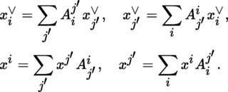
Memory aid:– Indices such as i, j, k refer to the old basis; primed indices such as i′, j′, k′ refer to the new basis and are written as superscripts for the change-of-basis matrix A or as subscripts for its inverse A − 1. The indices of the components of a vector are usually written as superscripts; the indices of the components of a covector are usually written as subscripts. The indices of a sequence of vectors are always subscripts; the indices of a sequence of covectors are always superscripts. This is motivated by “Einstein’s summation convention” (see Remark 4.2 in section 4.2.1).
If x ∈ E, x ∨ ∈ E ∨, the duality bracket of these two vectors is written as 〈x, x ∨〉. A change of basis in E and E ∨ may therefore be written as:

Let x = Σ i x i e i ∈ E and x∨ = Σ i e ∨ i x i ∨ ∈ E′. Then, x = Σ j′ x j′ e j′ and x ∨ = Σ j′ e ∨ j′ x j′ ∨, where:
Since
is commutative, we do not need to distinguish between left
-vector spaces and right
-vector spaces. Therefore, the duality bracket of x ∈ E, x
∨ ∈ E
∨ can also be written as 〈x
∨, x〉. For example, if
 is a differentiable function in some non-empty open subset Ω of E, then, at each point a of Ω, we have Df (a) ∈ E
∨ (see Lemma-Definition 1.4). If h
a
∈ E, it might seem more convenient to write (Df (a), h
a
) instead of (h
a
, Df (a)) for the quantity Df (a).h
a
, but the reverse notation is also perfectly justifiable (section 2.2.4
(IV)
).
is a differentiable function in some non-empty open subset Ω of E, then, at each point a of Ω, we have Df (a) ∈ E
∨ (see Lemma-Definition 1.4). If h
a
∈ E, it might seem more convenient to write (Df (a), h
a
) instead of (h
a
, Df (a)) for the quantity Df (a).h
a
, but the reverse notation is also perfectly justifiable (section 2.2.4
(IV)
).
(III) Recall the following fact ([P2], section 3.9.3(II)): let E
1, …, E
n
be normed vector spaces, each equipped with a norm |.|, and suppose that F is a semi-normed vector space equipped with a semi-norm |.|γ. The space
 of continuous n-linear mappings from E
1 × … × E
n
into F is a semi-normed vector space when equipped with the semi-norm ||.||γ defined for any mapping
of continuous n-linear mappings from E
1 × … × E
n
into F is a semi-normed vector space when equipped with the semi-norm ||.||γ defined for any mapping
 by:
by:
If F is a Hausdorff locally convex space whose topology is induced by the family of semi-norms (|.|γ)γ ∈ Γ ([P2], section 3.3.3), then
is a Hausdorff locally convex space when equipped with the family of semi-norms (|.|γ)γ ∈ Γ. This space is quasi-complete whenever F is quasi-complete ([P2], section 3.4.2
(II)).
Write
 for the space
whenever E
i
= E for all i ∈ {1, …, n}. An element u of
is said to be symmetric if, for all (h
1, …, h
n
) ∈ E
n
and every permutation
for the space
whenever E
i
= E for all i ∈ {1, …, n}. An element u of
is said to be symmetric if, for all (h
1, …, h
n
) ∈ E
n
and every permutation
 ,we have u(h
1, …, h
n
) = u(h
σ(1), …, h
σ(n)). The set of symmetric elements of
is written as
,we have u(h
1, …, h
n
) = u(h
σ(1), …, h
σ(n)). The set of symmetric elements of
is written as
 and is a vector subspace of
; this subspace is equipped with the family of semi-norms (||.||γ)γ ∈ Γ. If h ∈ E and
and is a vector subspace of
; this subspace is equipped with the family of semi-norms (||.||γ)γ ∈ Γ. If h ∈ E and
 , set:
If E is finite-dimensional, then we have the following canonical isomorphism:
(IV) See also the conventions (C1) (section 2.2.1 (III) , p. 55), (C2) (section 2.2.2 (III) , p. 58), (C3) (section 6.2.1 (II), p. 253).
1.2.2 Fréchet differential
(I) Let E, F be two locally convex spaces and ϕ a mapping from U into F, where U is some neighborhood of 0 in E.
Definition 1.2
We say that ϕ is tangent to 0 if, for every neighborhood W of 0 in F
, there exists a balanced neighborhood V ⊂ U of 0 in E such that, for every
 with sufficiently small | t |, we have ϕ (tV) ⊂ o (t) W (where
 ).
).
Proof
(i) With the notation of Definition 1.2, we have
 , so ϕ (V) ⊂ {0} and ϕ = 0. (ii): exercise.
From this lemma, we immediately deduce the following claim (ii):
Lemma-Definition 1.4
Let a be some point of E, U some neighborhood of 0 in E , and f : U + a → F some mapping where a + U := {a + x : x ∈ U}.
-
i)
We say that f is (Fréchet) differentiable at a if there exists a continuous linear mapping
 such that the mapping h ↦ f (a + h) − f (a) − L.h (defined in U) is tangent to 0.
- ii) This mapping L is uniquely determined.
- iii) This mapping is written as L = D f (a) (or L = d a f or L = f′ (a)) and is called the (Fréchet) differential of f at the point a.
The notion of the Fréchet differential is especially fruitful when E is a normed vector space. In this case, if A is an open subset of E, F is a locally convex space, a is a point of A, and f : A → F is a mapping, then f is differentiable at a with differential D f (a) at this point if and only if
The canonical isomorphism
 ([P2], section 3.3.8) reintroduces the usual notion of derivative, including the notion of a “complex derivative” when
([P2], section 4.2.1, Theorem-Definition 4.45). Indeed, keeping the same notation as before, we obtain:
([P2], section 3.3.8) reintroduces the usual notion of derivative, including the notion of a “complex derivative” when
([P2], section 4.2.1, Theorem-Definition 4.45). Indeed, keeping the same notation as before, we obtain:
Corollary-Definition 1.5
If
 , the function f : U + a → F is differentiable at the point
 (in the above sense) if and only if it is differentiable at a (in the usual sense of differentiability of functions of one real or complex variable), in which case the element
 of F is the derivative of f at a.
Theorem 1.6
(Rolle) Let [a, b] be a compact interval of
 with non-empty interior and suppose that
 is a continuous function in [a, b] that is differentiable in ]a, b[ and which satisfies φ (a) = φ (b). Then, there exists c ∈ ]a, b[ such that
 .
.
Proof
If φ is constant in [a, b], then it is differentiable and has zero derivative on ]a, b[. otherwise, it attains its lower and upper bounds ([P2], section 2.3.7, Theorem 2.42). one of these values is attained at some point c ∈ ]a, b[, which must therefore satisfy
(exercise).
If f is differentiable at the point a, then it is also continuous at this point (exercise). Let A be a non-empty open subset of E and write
 for the set of mappings from A into F that are differentiable at the point a ∈ A. The mapping
 is known as the differentiation operator at the point a and is
-linear.
is known as the differentiation operator at the point a and is
-linear.
Definition 1.7
Let
 . The rank rk (D
f (a)) ([P1],section 3.1.10,
Definition 3.38
(ii)) is said to be the rank of f at the point a and is written as rk
a
(f).
. The rank rk (D
f (a)) ([P1],section 3.1.10,
Definition 3.38
(ii)) is said to be the rank of f at the point a and is written as rk
a
(f).
(II) Let E be a real Hilbert space, A some non-empty open subset of E, and
 a function that is differentiable at the point a ∈ A. Then, Df (a) ∈ E
∨. By Riesz’s theorem ([P2], section 3.10.2(IV), Theorem 3.15(1)), there exists some uniquely determined element x
* ∈ E such that Df (a) coincides with the linear form h ↦ 〈x
∗| h〉.
a function that is differentiable at the point a ∈ A. Then, Df (a) ∈ E
∨. By Riesz’s theorem ([P2], section 3.10.2(IV), Theorem 3.15(1)), there exists some uniquely determined element x
* ∈ E such that Df (a) coincides with the linear form h ↦ 〈x
∗| h〉.
(III) Some of the classical results of differential calculus ([DIE 93], Volume 1, Chapter 8) are reproduced below. A few are stated in a slightly more general form than the cited reference; however, the reasoning is identical and entirely straightforward in each case.
Theorem 1.9
(chain rule) Let E, F be normed vector spaces, G a locally convex space, A some non-empty open subset of E
, a some point of A, B an open subset of F containing f (a),
, and
 . Then,
 and
and

Example 1.10
Let E be a Banach space. The set
 of continuous linear bijections is open in
 ([P2],
section 3.4.1
(II),
Lemma 3.50
). The mapping u ↦ u
− 1 from
([P2],
section 3.4.1
(II),
Lemma 3.50
). The mapping u ↦ u
− 1 from
 onto
is differentiable, and its differential at the point u
0 is the continuous linear mapping s ↦ − u
0
− 1 ∘ s ∘ u
0 (from
into
). The reader may wish to prove this result as an exercise or refer to
Lemma 1.24
of
section 1.2.5
(II).
onto
is differentiable, and its differential at the point u
0 is the continuous linear mapping s ↦ − u
0
− 1 ∘ s ∘ u
0 (from
into
). The reader may wish to prove this result as an exercise or refer to
Lemma 1.24
of
section 1.2.5
(II).
(IV) Let E 1, …, E n be normed vector spaces. Then, E = E 1 × … × E n can be canonically equipped with the structure of a normed vector space ([P2], section 3.4.1 (I)). Let A be a non-empty open subset of E and suppose that a = (a 1,…,a n ) ∈ A. Suppose further that F is a locally convex space. If f : A → F : (x 1, …, x n ) ↦ f (x 1, …, x n ) is differentiable at the point a, then the mapping

is defined in some open neighborhood of 0 in E
i
and differentiable at 0 for all i ∈ {1, …n} (exercise); its differential at this point is written as D
i
f (a) (or d
i
f (a) or
 ).
).
Given the conditions stated above, the differential D f (a) can be expressed in terms of the partial differentials D i f (a) as follows:
where h = (h
1, …, h
n
). If
 , the element ∂
i
f (a) = D
i
f (a).1 ∈ F is called the i-th partial derivative of f at the point a; writing (e
i
)1 ≤ i ≤ n
for the canonical basis of
, the element ∂
i
f (a) = D
i
f (a).1 ∈ F is called the i-th partial derivative of f at the point a; writing (e
i
)1 ≤ i ≤ n
for the canonical basis of
 , we have
If
, the existence of the partial differentials D
i
f (a)(i = 1, …, n) does not imply the existence of the differential D
f (a) (however, see Theorem 1.16(ii)).
If
 for all j ∈{1, …, n} and
 , then the linear mapping D
f (a) can be represented with respect to the canonical bases by the Jacobian matrix [∂
i
f
j
(a)]1 ≤ i ≤ m, 1 ≤ j ≤ n
, where f = (f
1, …, f
n
). If n = m, the determinant of this matrix is called the Jacobian of f at the point a and is written as
, then the linear mapping D
f (a) can be represented with respect to the canonical bases by the Jacobian matrix [∂
i
f
j
(a)]1 ≤ i ≤ m, 1 ≤ j ≤ n
, where f = (f
1, …, f
n
). If n = m, the determinant of this matrix is called the Jacobian of f at the point a and is written as
 .
.
(V) In the following,
. Let F be a locally convex space and |.|γ a continuous semi-norm on F.
Theorem 1.12
(mean value theorem, 1st version) Let I = [α, β] be a compact interval of
, f a continuous mapping from I into F and φ
γ a continuous mapping from I into
. Suppose that there exists a countable subset
 such that f and φ
γ both have a derivative at every point ξ ∈ D and
such that f and φ
γ both have a derivative at every point ξ ∈ D and
 . Then, | f(β) − f(α)|
γ
≤ φ
γ
(β) − φ
γ
(α).
. Then, | f(β) − f(α)|
γ
≤ φ
γ
(β) − φ
γ
(α).
Let E be a normed vector space with norm |.|. With the notation of [1.3] (with n = 1), we have the following result:
Theorem 1.13
(mean value theorem, 2nd version) Let f be a mapping taking values in F that is defined and continuous in some neighborhood of the closed segment S = [a, a + h] joining the points a, a + h of E ([P2], section 3.3.1 ). Suppose that f is differentiable at every point of S.
-
i)
Given any subset Θ of [0, 1] with countable complement in [0, 1],
-
ii)
Let
. Given any subset Ξ of [a, a + h] with countable complement in [a, a + h], we have | f (a + h) − f (a) − L.h |γ ≤ M
γ. | h | with M
γ = sup
x ∈ Ξ || D
f (x) − L ||γ
. In particular, if M
γ = sup
x ∈ Ξ || D
f (x) − D
f (a)||γ
, then
-
iii)
Let
 . There exists θ ∈ ]0, 1[ such that


Proof
Let g :[0, 1] ↦ F : t ↦ f (a + t.h). By Theorem 1.9,
 , so
, so
 , where N
γ = sup
t ∈ Θ || D
f (a + t.h)||γ. The upper bound of (i) is therefore obtained by applying Theorem 1.12 with f replaced by g and φ
γ (t) = N
γ.t. | h |.
, where N
γ = sup
t ∈ Θ || D
f (a + t.h)||γ. The upper bound of (i) is therefore obtained by applying Theorem 1.12 with f replaced by g and φ
γ (t) = N
γ.t. | h |.
- (ii) Can be deduced by applying (i) to the function ξ ↦ f (ξ) − L. (ξ − x).
-
(iii) Let
. Since g (0) = g (1) = 0, Rolle’s theorem (Theorem 1.6) implies the existence of a number θ ∈ ]0, 1[ such that
 .
.
Theorem 1.13 has the following two corollaries:
1.2.3 Mappings of class Cp
In this section,
.
(I) Let E be a normed vector space and suppose that F is a locally convex space. Write
for the space of continuous n-linear mappings from E
n
into F equipped with the family of semi-norms [1.3].
Let A be a non-empty open subset of E and suppose that f : A → F is a mapping. We say that f is of class C
0 if it is continuous in A. We say that it is of class C
1 if it is differentiable in A and its differential
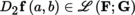
 is continuous. We say that f is twice differentiable (respectively is of class C
2 )in A if its differential
D
f is differentiable (respectively is of class C
1) in A. At any given point a ∈ A, the second differential D (D
f)(a), written as D
2
f (a), is an element of
is continuous. We say that f is twice differentiable (respectively is of class C
2 )in A if its differential
D
f is differentiable (respectively is of class C
1) in A. At any given point a ∈ A, the second differential D (D
f)(a), written as D
2
f (a), is an element of
 ; this space can be identified with
 by ([P2], section 3.9.3(II)). Similarly, we may recursively define a p-times differentiable mapping (respectively a mapping of class C
p
)in A for any integer p ≥ l, as well as the p-th order differential
by ([P2], section 3.9.3(II)). Similarly, we may recursively define a p-times differentiable mapping (respectively a mapping of class C
p
)in A for any integer p ≥ l, as well as the p-th order differential
 for any point a ∈ A. We say that f is of class C
∞ if f is of class C
p
for every p ≥ l. We write
for any point a ∈ A. We say that f is of class C
∞ if f is of class C
p
for every p ≥ l. We write
 for the
-vector space of mappings of class C
p
from A into F (0 ≤ p ≤ ∞).
for the
-vector space of mappings of class C
p
from A into F (0 ≤ p ≤ ∞).
From ([DIE 93], Volume 1, (8.12.1), (8.16.6)), mutatis mutandis, we have the following result:
Theorem 1.16
Let F be a locally convex space.
i) (Schwarz’s theorem) Let E be a normed vector space, A some non-empty open subset of E and f : A → F a p-times differentiable mapping (p ≥ 2) at some point a ∈ A. Then, the differential D
p
f (a) is symmetric and therefore belongs to
 .
.
ii) Let E 1, …, E n be normed vector spaces (n ≥ 2) and suppose that A is a non-empty subset of E 1 × … × E n . For any p such that 1 ≤ p ≤ ∞, f is of class C p in A if and only if the n p partial derivatives of order p of f exist and are continuous in A (where n ∞ := ∞).
By Theorem 1.16(ii), a mapping f from a non-empty open subset Ω of
 into
into
 is of class C
p
if and only if its n
p
partial derivatives exist and are continuous, i.e.
is of class C
p
if and only if its n
p
partial derivatives exist and are continuous, i.e.
 ([P2], section 4.3.1
(I)).
([P2], section 4.3.1
(I)).
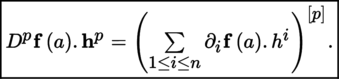
(II) In the context of Theorem 1.16(i), when
 , introducing “symbolic powers” gives us an easy way to express D
p
f (a).h
p
(with the notation of section 1.2.1
(III)) in terms of the partial derivatives of order p:
, introducing “symbolic powers” gives us an easy way to express D
p
f (a).h
p
(with the notation of section 1.2.1
(III)) in terms of the partial derivatives of order p:

where D i denotes the partial differential in the i-th variable. Writing h = (h 1, …, h n ), we have D 2 f (a).h 2 = Σ1 ≤ i,j ≤ n ∂ i ∂ j f (a).h i h j 4 . This can be expressed as (Σ1 ≤ i ≤ n ∂ i f (a).h i )[2] by developing the latter like any other squared parentheses and replacing (∂ i f (a).h i ) (∂ j f (a).h j ) by ∂ i ∂ j f (a).h i h j . With the same conventions, we can continue inductively to obtain the following result:
If
(i = 1, …, n),
 , and
, and
 is twice differentiable at some point a of A, then the matrix H f (a) = (∂
i
∂
j
f (a))1 ≤ i,j ≤ n
is called the Hessian matrix
5
of f at the point a. Identifying the vectors of
with the columns of this matrix gives D
2
f (a).h
2 = h
T
.H f (a).
h
.
is twice differentiable at some point a of A, then the matrix H f (a) = (∂
i
∂
j
f (a))1 ≤ i,j ≤ n
is called the Hessian matrix
5
of f at the point a. Identifying the vectors of
with the columns of this matrix gives D
2
f (a).h
2 = h
T
.H f (a).
h
.
(III) Suppose that l ≤ p ≤ ∞. The following results can be shown by induction (exercise). The composition of two mappings of class C p is also of class C p . If E is a normed vector space, A some non-empty open subset of E, F and G locally convex spaces, u a continuous linear mapping from F into G and f : A → F a mapping of class C p in A, then u ∘ f is of class C p in A and D p (u ∘ f) = u ∘ D p f. With the same hypotheses on E and A, if F 1, F 2, and G are locally convex spaces, [.,.] is a continuous bilinear mapping from F 1 × F 2 into G, and f i is a mapping of class C p from A into F i for i = 1, 2, then [f1, f2] is of class C p from A into G and the so-called Leibniz rule holds:

(IV) Nemytskii Operator
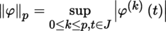
Let F be a Banach space, J a compact interval of
with non-empty interior, and
 the space of mappings of class C
p
(p ≥ 1) from J into F. Then,
is a Banach space when equipped with the norm
the space of mappings of class C
p
(p ≥ 1) from J into F. Then,
is a Banach space when equipped with the norm
(exercise). Let U be an open neighborhood of 0 in F, f : U × J → F a mapping of class C
p
and
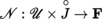 the so-called Nemytskii operator, defined by
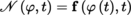 , where
 .
.
Theorem 1.17
The Nemytskii operator
 is of class C
p
and
is of class C
p
and

Proof
The operator
is the composition
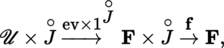
where
 is the evaluation operator defined by ev (φ, t) = φ(t). But ev is of class C
p
and
is the evaluation operator defined by ev (φ, t) = φ(t). But ev is of class C
p
and

(exercise
*
: see [ABR 83], Proposition 2.4.17). Since f is of class C
p
, so is
by (III), and [1.10] follows from [1.5].
Remark 1.18
The operator
defined above is stated slightly more generally than the classical Nemytskii operator, which does not allow t to vary (to recover the classical case, set the increase τ to 0 in
[1.10]
).
1.2.4 Taylor’s formulas
Throughout this section,
, and F denotes a quasi-complete locally convex space. Readers who are only interested in mappings taking values in a Banach space (see Remark 1.1) may skip (I) and (II) below.
(I) Mackey Convergence Let B be a balanced convex subset (also known as an “absolutely convex” subset ([KÖT 79], Volume 1, section 16.1(2))) that is closed and bounded in F, and write F 1 = ∪ n = 1 ∞ nB. The gauge of p B of B in F 1 ([P2], section 3.3.2 (I)) is a norm on F 1 (exercise) and F 1 is a Banach space, written as F B , when equipped with this norm.
Mackey convergence of a sequence of elements of F implies the usual notion of convergence and is equivalent to it whenever F is a Fréchet space or the strong dual of an infrabarreled Schwartz space ([HOG 71], p. 8, Example 3), such as the distribution spaces studied in ([P2], section 4.4.1).
(II) Generalized Riemann integral To state Taylor’s formulas in a general framework, it will be useful to introduce the generalized Riemann integral of a function of a real variable taking values in a quasi-complete locally convex space 6 .
Lemma-definition 1.20
Let F be a quasi-complete locally convex space, I a non-empty open interval of
, c some point of I and f : I → F a continuous mapping.
- i) There exists a unique differentiable mapping ∫ f : I → F such that (∫ f)(c) = 0 and (∫ f)′ = f .
- ii) Let a, b ∈ I. Write ∫ a b f(t)dt = (∫ f)(b) − (∫ f)(a); this quantity is called the (generalized) Riemann integral of f from a to b.
- iii) If f : [a, b] → F is Lipschitz, consider the points a = t 0 < t 1 < … < t n = b of the interval [a, b], and the Riemann sum S n = ∑ i = 0 n − 1(t i + 1 − t i )f(t i ). If n → ∞ and | t i + 1 − t i | → 0 for all i ∈ {1, …, n − 1}, then S n → ∫ a b f(t)dt in the sense of Mackey convergence.
If F is a Banach space, this recovers the classical notion of the integral of a continuous function. The integration operator ∫ a b defined above satisfies the usual properties ([KRI 97], Chapter 1, Corollary 2.6). In particular, we have the following result:
Theorem 1.21
(integral mean value theorem) Let I = [α, β] be a compact interval of
and let f : I → F be a continuous mapping. For every continuous semi-norm |.|γ of F,

Proof
Let g(t) = ∫
α
t
f(t). dt. By the definition of the integral, g is differentiable in I and
 , where
 . Applying the mean value theorem (Theorem 1.12) to g therefore gives the desired inequalities.
(III) Taylor’s formulas Let E be a normed vector space with norm |.|, A some non-empty open subset of E and F a quasi-complete locally convex space whose topology is defined by a family of semi-norms (|.|γ)γ ∈ Γ. With the conventions of section 1.2.1 and p ≥ l, we have the following result:
Theorem 1.22
-
i)
Let f : A → F be a mapping of class C
p
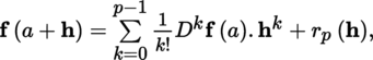
in A. If the segment [a, a + h] is contained in A, then f satisfies Taylor’s formula
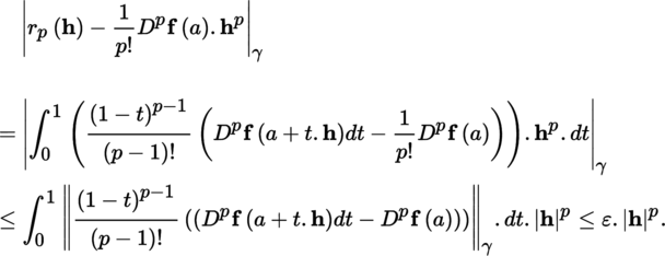
where the residual r p (h) is the (Laplace residual) integral -
ii) As | h | → 0, we can alternatively express the residual in the form of Young’s residual:
-
iii)
Let γ ∈ Γ and suppose that there exists some real number M > 0 such that sup
x ∈]a,a + h[ || D
p
f (x)||γ ≤ M. Then, | r
p
(h)|γ is upper bounded by the Lagrange residual:
-
iv)
If
 , suppose that f is of class C
p − 1 in A and admits a differential of order p, D
p
f (x), at every point of the open segment ]a, a + h[. The Lagrange residual can be expressed as follows: there exists θ ∈ ]0, 1[ such that
, suppose that f is of class C
p − 1 in A and admits a differential of order p, D
p
f (x), at every point of the open segment ]a, a + h[. The Lagrange residual can be expressed as follows: there exists θ ∈ ]0, 1[ such that
Proof
-
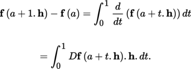
i) For p = 1,
For p = 2, we can simply evaluate the above integral by parts. This integral is of the form ∫0 1 u. dv with u = D f (a + t h).h and v = 1 − t; hence, [u. v]0 1 − ∫0 1 v. d u = D f(a) + ∫0 1(1 − t)D 2 f(a + t h). h 2. dt. Continuing inductively gives (i). -
ii)
Since D
p
f is continuous, for all ε > 0, there exists a real number r
γ > 0 such that || D
p
f (a + t.h) − D
p
f (a)||γ ≤ p!ε whenever | h | ≤ r and 0 ≤ t ≤ 1. The first inequality of the integral mean value theorem (Theorem 1.21) then implies:
-
iii) This again follows from (i) and the integral mean value theorem, since
-
iv) First, consider the case of a function g that is defined and of class C
p − 1 in some open neighborhood of a compact interval [a, b] of
and assumed to have a p-th derivative g
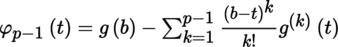
(p) (t) in ]a, b[. Set
and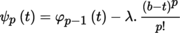 , where λ is chosen so that ψ
p
(a) = 0. Since ψ
p
(b) = 0, Rolle’s theorem (Theorem 1.6) implies that there exists a point c ∈ ]a, b[ such that ψ
p
(p) (c) = 0, and hence
, where λ is chosen so that ψ
p
(a) = 0. Since ψ
p
(b) = 0, Rolle’s theorem (Theorem 1.6) implies that there exists a point c ∈ ]a, b[ such that ψ
p
(p) (c) = 0, and hence
We now simply need to apply this result to the mapping g (t) = f (a + t.h), t ∈ [0, 1].

Corollary 1.23
Let E be a real normed vector space, A some non-empty subset of E,
a mapping of class C
p
(2 ≤ p ≤ ∞) and a some point of A.
- i) For f to have a relative minimum (or local minimum) at the point a, the smallest integer n ≤ p such that D n f (a) is non-zero (if any such integer n exists) must necessarily be even; furthermore, D n f (a).h ≥ 0 for every non-zero vector h ∈ E.
- ii) Conversely, if A is convex, n ≤ p is even, D i f (a) = 0 for all i ∈ {1, …, n − 1}, and D n f (x) .h n > 0 for all x ∈ A and every h ≠ 0, then f has a strict relative minimum at the point a.
- iii) If D i f (a) = 0 for all i ∈ {1, …, n − 1}, n ≤ p is even, and there exists ε > 0 such that D n f (x).h n > ε | h | n for every x ∈ A and every h ≠ 0, then f has a strict relative minimum at the point a (if E is finite-dimensional, this sufficient condition is still valid with ε = 0).
Proof
i) follows from Taylor’s formula with Young’s residual; ii) and iii) follow from Taylor’s formula with the Lagrange residual. If E is finite-dimensional, the unit sphere
 is compact by Riesz’s theorem ([P2], section 3.2.3, Theorem 3.11); thus,
 is compact by Tychonov’s theorem ([P2], section 2.3.7, Theorem 2.43) and D
n
f (x).h
n
has a minimum ε > 0 in
(ibid., Theorem 2.39).
is compact by Tychonov’s theorem ([P2], section 2.3.7, Theorem 2.43) and D
n
f (x).h
n
has a minimum ε > 0 in
(ibid., Theorem 2.39).
(IV) If E = E
1 × … × E
n
, where each E
i
is a normed vector space, let α be the multi-index (α
1, …, α
n
),
 (i ∈ {1, …, n}). Define

the operator D
α
is called the partial differential of order α. If each E
i
is equal to
, write ∂
α
for D
α
([P2], section 4.3.1
(I)). Let U be an open neighborhood of a in E and suppose that the function f : U → F is of class C
p
in U. Then, Taylor’s formula can be rewritten as follows:
1.2.5 Analytic functions
(I) Power series
Let E be a normed vector space with norm |.| and suppose that F is a Hausdorff quasi-complete locally convex space (see Remark 1.1 for the case where F is normable). With the notation of section 1.2.1, let
 be the
-vector space of formal power series S = ∑
p
S
p
, where S
p
= c
p
.X
p
and
be the
-vector space of formal power series S = ∑
p
S
p
, where S
p
= c
p
.X
p
and
 . Let (|.|γ)γ ∈ Γ be a family of semi-norms which induces the topology of F and let r > 0; we write that ‖S‖
γ, r
= ∑
p
r
p
‖c
p
‖
γ
and
. Let (|.|γ)γ ∈ Γ be a family of semi-norms which induces the topology of F and let r > 0; we write that ‖S‖
γ, r
= ∑
p
r
p
‖c
p
‖
γ
and
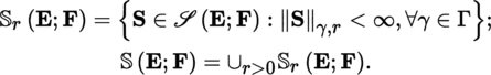
The set
 is a
-vector space called the space of convergent power series. If
is a
-vector space called the space of convergent power series. If
 , we say that
 is the radius of convergence of S. Suppose that ρ (S) > 0; if we replace the indeterminate X with an element h ∈ E such that | h | < ρ (S), then the family c
p
.h
p
is summable ([P2], section 3.2.1
(III)), as can be seen by adapting the proof of ([P2], section 3.4.1
(I), Theorem 3.41), and the mapping S : S ↦ S (h) is continuous in the open set | h | < ρ (S).If F is a Banach space and ρ (S) > 0, then the power series S is absolutely convergent in | h | < ρ (S) and normally convergent in | h | ≤ r′ for every r′ such that 0 < r′ < ρ (S) ([P2], section 4.3.2
(I)).
is the radius of convergence of S. Suppose that ρ (S) > 0; if we replace the indeterminate X with an element h ∈ E such that | h | < ρ (S), then the family c
p
.h
p
is summable ([P2], section 3.2.1
(III)), as can be seen by adapting the proof of ([P2], section 3.4.1
(I), Theorem 3.41), and the mapping S : S ↦ S (h) is continuous in the open set | h | < ρ (S).If F is a Banach space and ρ (S) > 0, then the power series S is absolutely convergent in | h | < ρ (S) and normally convergent in | h | ≤ r′ for every r′ such that 0 < r′ < ρ (S) ([P2], section 4.3.2
(I)).
(II) Analytic functions
Let A be a non-empty open subset of E. We say that a function f from A into F is analytic (or is a mapping of class C
ω
) if, for each point a ∈ A, there exists a convergent series
, denoted by f
a
, such that f (a + h) = f
a
(h) for every h ∈ E with sufficiently small norm. This definition generalizes ([P2], section 4.3.2
(I), Definition 4.74). Write
 for the
-vector space of analytic functions from A into F. If
and
for the
-vector space of analytic functions from A into F. If
and
 , then f is of class C
∞ in A, and so is each of its differentials D
p
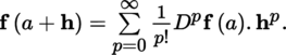
f (p ≥ 1). Every mapping
admits the following Taylor series expansion at the point a, which converges in | h | < ρ(f
a
):
, then f is of class C
∞ in A, and so is each of its differentials D
p
f (p ≥ 1). Every mapping
admits the following Taylor series expansion at the point a, which converges in | h | < ρ(f
a
):
If | a | < ρ(f a ), then the radius of convergence of the Taylor expansion of f at the point a is greater than or equal to ρ (f a ) − | a |. If A = E and ρ (f a ) = +∞, then the function f is said to be entire.
Let E, F be Banach spaces, G a quasi-complete locally convex space, A an open subset of E, f : A → F an analytic function, B an open subset of F containing f (A) and g : B → G an analytic function. Then, g ∘ f is analytic (exercise); see ([BOU 82a], 3.2.7), ([WHI 65], p. 1079).
The principle of analytic continuation ([P2], section 4.3.2, Theorem 4.76) can be generalized as follows (exercise: see [WHI 65], p. 1080): let E and F be two Banach spaces, Ω a connected open subset of E and f, g two analytic functions from Ω into F. If f and g coincide in any non-empty open subset of Ω, then they must be equal.
Lemma 1.24
Let E be a Banach space and write
for the subset of invertible operators in
. Let
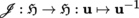 . The mapping
 is analytic and satisfies
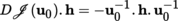 for every
 .
.
Proof
We know that
is open in
([P2], section 3.4.1
(II), Corollary 3.49). Let
and
 . We have u
0 + s = u
0 (1
E
− v), where v = − u
− 1
s. If || v || < 1, then 1
E
− v is invertible with inverse Σ
n ≥ 0 v
n
(ibid.). Hence, if
. We have u
0 + s = u
0 (1
E
− v), where v = − u
− 1
s. If || v || < 1, then 1
E
− v is invertible with inverse Σ
n ≥ 0 v
n
(ibid.). Hence, if
 , u
0 + s has inverse ∑
n ≥ 0(− u
0
− 1. s)
n
u
0
− 1, which shows that
is analytic. Furthermore, ∑
n ≥ 0(− u
0
− 1. s)
n
u
0
− 1 = u
0
− 1 − u
0
− 1. s. u
0
− 1 + o(‖s‖).
, u
0 + s has inverse ∑
n ≥ 0(− u
0
− 1. s)
n
u
0
− 1, which shows that
is analytic. Furthermore, ∑
n ≥ 0(− u
0
− 1. s)
n
u
0
− 1 = u
0
− 1 − u
0
− 1. s. u
0
− 1 + o(‖s‖).
(III) Holomorphic functions
Let E be a normed complex vector space with norm |.|, A some non-empty open subset of E, and F a complex quasi-complete locally convex space. Goursat’s theorem ([P2], section 4.2.4, Proposition 4.56) can be generalized as follows ([BOU 82a], 3.1.1): the function f : A → F is analytic if and only if it is holomorphic (i.e. complex-differentiable). If this condition is satisfied for E = E
1 × … × E
n
, let a =(a
1,…, a
n
) ∈ A, r = (r
1, …, r
n
), where r
i
> 0, and
 , where α is the multi-index (α
1,…, α
n
). The Cauchy inequalities ([P2], section 4.3.2
(II), Lemma-Definition 4.78(2)) can be generalized as follows (exercise): for r
α
≔ r
1
α
1
…r
n
α
n
,
, where α is the multi-index (α
1,…, α
n
). The Cauchy inequalities ([P2], section 4.3.2
(II), Lemma-Definition 4.78(2)) can be generalized as follows (exercise): for r
α
≔ r
1
α
1
…r
n
α
n
,
Hence ([P2], section 4.3.2 (II), Theorem-Definition 4.81(3)), if f is entire in E and bounded in F, then it must be constant (Liouville’s theorem). The statement of Hartogs’ theorem ([P2], section 4.3.2 (II), Corollary 4.80) also holds, mutatis mutandis, for a function f : A → F, where A is an open subset of E 1 × … × E n , and each E i is a complex normed vector space: any such function is analytic if and only if it is analytic in each of its variables when the others are held fixed.
Proof
-
1) Let us begin by showing the result by contradiction when
 . Suppose that f has a maximum in A. By translation, we may assume that 0 ∈ A and that this maximum is attained at 0. Let c
0 = f (0). If f is not constant, then there exists b
m
≠ 0 such that f (z) = c
0 (1 + b
m
z
m
+ z
m
.h (z)), where h is holomorphic in A and satisfies h (0) = 0. Choose r > 0 such that | z | ≤ r implies z ∈ A and
. Suppose that f has a maximum in A. By translation, we may assume that 0 ∈ A and that this maximum is attained at 0. Let c
0 = f (0). If f is not constant, then there exists b
m
≠ 0 such that f (z) = c
0 (1 + b
m
z
m
+ z
m
.h (z)), where h is holomorphic in A and satisfies h (0) = 0. Choose r > 0 such that | z | ≤ r implies z ∈ A and
 . Let
. Let
 be such that
 . For z = re
it
, we have
. For z = re
it
, we have
which is a contradiction. -
2) In the case where
 , we can similarly argue by contradiction by assuming that there exist z
0, z
1 ∈ A such that | f (z) |γ ≤ | f (z
0)|γ for all z ∈ A and | f (z
1)|γ < | f (z
0)|γ. Let
, we can similarly argue by contradiction by assuming that there exist z
0, z
1 ∈ A such that | f (z) |γ ≤ | f (z
0)|γ for all z ∈ A and | f (z
1)|γ < | f (z
0)|γ. Let
 and
and
 . Then, | η |γ = 1, where
 . By the Hahn–Banach theorem ([P2], section 3.3.4(II), Theorem 3.25), there exists a continuous linear form ξ ∈ F∨ extending η such that | ξ |
γ
= 1. Therefore, for all x ∈ A, | ξ ∘ f (z)| ≤ | f (z)|
γ
≤ | f (z
0)|γ = | ξ ∘ f (z
0)|, so ξ ∘ f is constant by (1). Hence, | ξ ∘ f (z
1) = | ξ ∘ f (z
0)| = | f (z
0)|γ and | ξ ∘ f (z
1)| ≤ | f (z
1)|γ < | f (z
0)|γ, contradiction.
. By the Hahn–Banach theorem ([P2], section 3.3.4(II), Theorem 3.25), there exists a continuous linear form ξ ∈ F∨ extending η such that | ξ |
γ
= 1. Therefore, for all x ∈ A, | ξ ∘ f (z)| ≤ | f (z)|
γ
≤ | f (z
0)|γ = | ξ ∘ f (z
0)|, so ξ ∘ f is constant by (1). Hence, | ξ ∘ f (z
1) = | ξ ∘ f (z
0)| = | f (z
0)|γ and | ξ ∘ f (z
1)| ≤ | f (z
1)|γ < | f (z
0)|γ, contradiction.
-
3) In the general case, let g (ξ) = f (z
0 + ξ (z − z
0)) and suppose that | f (z)|
γ
≤ | f (z
0)|
γ
for all z ∈ A. Then, g is holomorphic in
 for sufficiently small r > 0 and z sufficiently close to z
0. Therefore, | g (ξ)|
γ
≤ | f (z
0)|
γ
= | g (0)|γ, and g is constant in Ω by (2). Thus, g (0) = g (1), so f (z) = f (z
0). The set of z ∈ A satisfying this condition is non-empty, open and closed in A, and so must be equal to A ([P2], section 2.3.8).
for sufficiently small r > 0 and z sufficiently close to z
0. Therefore, | g (ξ)|
γ
≤ | f (z
0)|
γ
= | g (0)|γ, and g is constant in Ω by (2). Thus, g (0) = g (1), so f (z) = f (z
0). The set of z ∈ A satisfying this condition is non-empty, open and closed in A, and so must be equal to A ([P2], section 2.3.8).
1.2.6 The implicit function theorem and its consequences
(I) Banach–Caccioppoli fixed point theorem
Proof
- a) Uniqueness: If f (ξ) = ξ and f (ξ′) = ξ′, then d (f (ξ), f (ξ′)) = d (ξ, ξ′) and d (f (ξ), f (ξ′)) ≤ k.d (ξ, ξ′), so d (ξ, ξ′) ≤ k.d (ξ, ξ′), and thus (1 − k).d (ξ, ξ′) ≤ 0. Since 1 – k > 0, this implies that d (ξ, ξ′) = 0 and ξ = ξ′.
- b)
Existence: We will use the method of successive approximation: let (x
n
) be the sequence of elements of X defined from some arbitrary starting point x
0 ∈ X by the recurrence relation x
n + 1 = f (x
n
). For all n ≥ 0,
and so for all p ≥ 1, by the triangle inequality,
Hence, (x n ) is a Cauchy sequence. Since X is complete, (x n ) must have some limit ξ in X; but f is continuous, so ξ = f (ξ).

(II) Inverse mapping and implicit function theorems Below, we assume that 0 < p ≤ ω.
This definition can be localized in the obvious way as we did for homeomorphisms ([P2], section 2.3.4 (III)). Every diffeomorphism (respectively local diffeomorphism) is clearly a homeomorphism (respectively local homeomorphism). A local diffeomorphism of class C p is also known as an étale mapping of class C p (see [P2], section 5.3.2 (II)).
Proof
-
1)
Preliminary: Since
 is bijective, it is a linear homeomorphism by the Banach inverse operator theorem ([P2], section 3.2.3, Theorem 3.12(2)(i)). Hence, E and F are isomorphic and can be identified. We can also assume that D
f (a) = 1
E
(left-multiplying f by D
f (a)− 1 if necessary) and reduce to the case where a = 0 by translation. Let ϕ (x) = x − f (x). We have Dϕ (0) = 0, and, since Dϕ is continuous, there exists r > 0 such that
is bijective, it is a linear homeomorphism by the Banach inverse operator theorem ([P2], section 3.2.3, Theorem 3.12(2)(i)). Hence, E and F are isomorphic and can be identified. We can also assume that D
f (a) = 1
E
(left-multiplying f by D
f (a)− 1 if necessary) and reduce to the case where a = 0 by translation. Let ϕ (x) = x − f (x). We have Dϕ (0) = 0, and, since Dϕ is continuous, there exists r > 0 such that
 . The mean value theorem (Theorem 1.13) then implies that
 whenever | x | ≤ r, i.e. ϕ (B
r
c
(0)) ⊂ B
r/2
c
(0), where B
r
c
(0) ≔ {x ∈ E : | x | ≤ r}.
whenever | x | ≤ r, i.e. ϕ (B
r
c
(0)) ⊂ B
r/2
c
(0), where B
r
c
(0) ≔ {x ∈ E : | x | ≤ r}.
-
2)
Existence of an inverse mapping g: B
r/2
c
(0)) → B
r
c
(0):
Let y ∈ B r/2 c (0). We will show that there exists a unique element x ∈ B r c (0) such that f (x) = y. Let ψ y (x) = y + x − f (x). If and | x | ≤ r, then | ψ
у
(x)| ≤ r, so ψ
у
is a mapping from B
r
c
(0) into B
r
c
(0). For all x
1, x
2 ∈ B
r
c
(0),
and | x | ≤ r, then | ψ
у
(x)| ≤ r, so ψ
у
is a mapping from B
r
c
(0) into B
r
c
(0). For all x
1, x
2 ∈ B
r
c
(0),
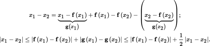
Since B r c (0) is a complete metric space ([P2], section 2.4.4(II), Lemma 2.77), Theorem 1.27 implies that ψ у has a unique fixed point in this set. This fixed point x satisfies y + x − f (x) = x, so f (x) = y, and x = g (y). -
3)
Continuity of g : For x
1, x
2 ∈ B
r
c
(0), we have:
Therefore, | x 1 − x 2 | ≤ 2 | f (x 1) − f (x 2)|. -
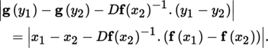
4)
Differentiability of g : Let y
i
= f (x
i
), y
i
∈ B
r/2
c
(0), x
i
∈ B
r
c
(0) (i = 1, 2). Then:
By taking sufficiently small r > 0, we can guarantee that || D f (x 2)− 1 || ≤ 1. Therefore,
which shows that g is differentiable and D g (y) = D f (x) − 1 in B r/2 (0). -
5)
Class of g : If
, the generalized Goursat theorem (section 1.2.5
(III)) implies that p = ω. Consider the case where
. Since D
f and g are continuous and
is analytic (Lemma 1.24),
 is continuous, and g is therefore of class C
1. By induction, it follows that if f is of class C
p
(1 ≤ p ≤ ∞), then g is of class C
p
.
is continuous, and g is therefore of class C
1. By induction, it follows that if f is of class C
p
(1 ≤ p ≤ ∞), then g is of class C
p
.
Suppose that f is analytic and therefore can be expressed as an absolutely convergent series f(x) = ∑ p c p . x p (| x | < ρ). By (1), c 0 = 0, c 1 = 1 E , so y = x + c 2.x 2 + c 3.x 3 + … According to a classical procedure dating back to Newton, x can be expressed in terms of y as a formal series x = y + ∑ i ≥ 2 d i . y i . The terms d i (i ≥ 2) are determined recursively: y 2 = x 2 + 2c 2.x 3 + …, y 3 = x 3 + …, which gives y = x + c 2. (y 2 − 2c 2.x 3) + …, and x = y − c 2 .y 2 + (2c2 2 − c3).y 3 + …, where c 2 2.y 3 := c 2 (y, c 2 (y, y)). We now need to study the convergence of this series. There exists K > 0 such that || c i || ≤ γ i , where . Thus, the majorant series
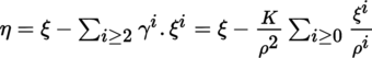
converges for | ξ | < ρ, with sum . As before, we can construct an inverse formal series ξ = η + ∑
i ≥ 2
δ
i
. η. Cauchy showed that this series has a non-zero radius of convergence as follows. By elementary arithmetic, the relation η = φ (ξ) is invertible and we may write ξ = ψ (η), for ξ ∈ ]−∞, ξ
1[, where
. As before, we can construct an inverse formal series ξ = η + ∑
i ≥ 2
δ
i
. η. Cauchy showed that this series has a non-zero radius of convergence as follows. By elementary arithmetic, the relation η = φ (ξ) is invertible and we may write ξ = ψ (η), for ξ ∈ ]−∞, ξ
1[, where
 , and η ∈ ]−∞, η
1[, where
, and η ∈ ]−∞, η
1[, where
 . It is easy to check that ψ can be expanded into an entire series in a neighborhood of 0 ([KNO 51], section 107). By section 1.2.5
(I), the formal series y + ∑
i ≥ 2
d
i
. y
i
therefore has a non-zero radius of convergence.
. It is easy to check that ψ can be expanded into an entire series in a neighborhood of 0 ([KNO 51], section 107). By section 1.2.5
(I), the formal series y + ∑
i ≥ 2
d
i
. y
i
therefore has a non-zero radius of convergence.


Theorem 1.30
(implicit function theorem) Let E, F and G be Banach spaces, A some non-zero open subset of E × F and f : A → G a mapping of class C
p
in A. Let (a, b) ∈ A be such that f (a, b) = 0 and suppose that
 is bijective. There exists some neighborhood U
0 of a in E such that, for every connected open set U ⊂ U
0 containing a, there is a unique continuous mapping u from U into F satisfying u(a) = b, (x, u (x)) ∈ A, and f (x, u(x)) = 0 for all x ∈ U. Furthermore, u is of class C
p
in U and, for all x ∈ U,
is bijective. There exists some neighborhood U
0 of a in E such that, for every connected open set U ⊂ U
0 containing a, there is a unique continuous mapping u from U into F satisfying u(a) = b, (x, u (x)) ∈ A, and f (x, u(x)) = 0 for all x ∈ U. Furthermore, u is of class C
p
in U and, for all x ∈ U,

Proof
-
1)
Existence of an implicit function: Since D
2
f (a, b) is bijective, it is an isomorphism from F onto G, and we may consider that F = G; furthermore, replacing f by D
2
f (a, b)− 1.f if necessary, we may assume that D
2
f (a, b) = 1
F
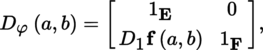
. Let φ : A → E × F :(x, y) ↦ (x, f (x, y)). We have
so D φ (a, b) is invertible in . By Theorem 1.29, φ is a local diffeomorphism of class C
p
and admits an inverse local diffeomorphism ψ of class C
p
.
. By Theorem 1.29, φ is a local diffeomorphism of class C
p
and admits an inverse local diffeomorphism ψ of class C
p
.
Write ψ (x, z) = (x, h (x, z)), where h is defined and of class C p in some neighborhood of (a, b) and takes values in F. Finally, set u (x) = h (x, 0). Then, u is of class C p in some neighborhood of a and takes values in F. Thus, there exists some neighborhood U 0 of a in E such that, for all x ∈ U 0,
and u (a) = h (a, 0),so (a, u (a)) = ψ (a, 0) = φ − 1 ((a, 0)) = (a, b), and therefore u (a) = b. Hence, u is an “implicit function” of class C p . -
2)
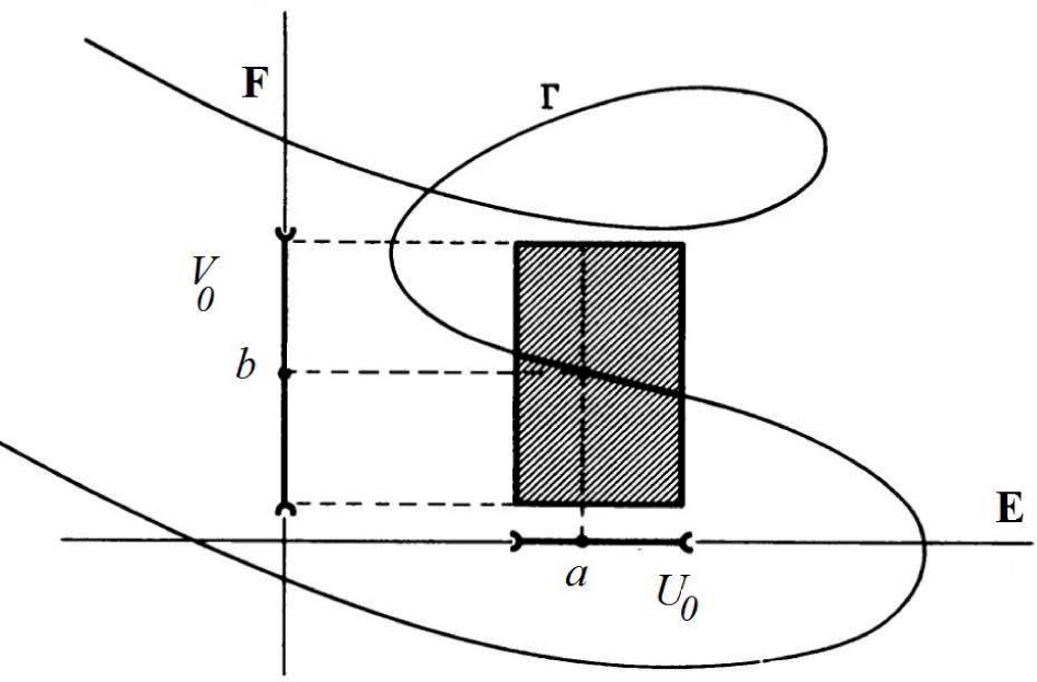
Uniqueness of the implicit function: Since φ is a local homeomorphism, there exist a neighborhood U′0 of a and a neighborhood V
0 of b such that there is a unique (x, y) in U′0 × V
0 satisfying φ (x, y) = (x, 0) (see Figure 1.1, where Γ is the graph of f). We may assume that U′0 is the same U
0 as above (replacing U
0 by U
0 ∩ U′0 if necessary).
If a continuous mapping v : U 0 → F satisfies v (a) = b and f (x, v(x)) = 0 for all x ∈ U 0, then we may assume that v(x) ∈ V 0 for all x ∈ U 0, further reducing the neighborhood U 0 of a if necessary. We may similarly assume that u, like v, is defined in U 0. Let U ⊂ U 0 be a connected neighborhood of a and suppose that M = {x ∈ U : u (x) = v (x)}. Then, a ∈ M and M is closed in U ([P2], section 2.3.3 (II), Lemma 2.30). We will show that M is also open in U. By the hypotheses, the mapping x ↦ D 2 f(x, u (x)) is continuous and D 2 f (a, b) = 1 F , so (again reducing the neighborhood U 0 if necessary) we may assume that D 2 f (x, u(x)) is invertible for all x ∈ U 0. Let a′ ∈ M. There exist a neighborhood U a′ ⊂ U of a′ and a neighborhood V a′ ⊂ V 0 of b′ = u (a′) such that, for all x ∈ U a′, u (x) is the only solution y of f (x, y) = 0 satisfying y ∈ V a′ . Given that v is continuous at a′ and v (a′)= u (a′), there exists a neighborhood W ⊂ U a′ of a′ such that v (x) ∈ V a′ whenever x ∈ W. Therefore, v (x) = u (x) for all x ∈ W, which proves that M is open. The set M is non-empty, open, and closed in the connected space U, which implies that M = U ([P2], section 2.3.8). -
3)
Calculation of D
u(x): Since f(x, u(x)) = 0 in U, the chain rule (Theorem 1.9) implies that
which gives us [1.16].


Remark 1.31
-
i)
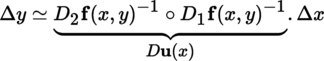
The implicit function theorem answers the following question: what condition makes it possible to express y = b + Δy uniquely as a function of x = a + Δx (so that y = u (x)) whenever f (x, y) = 0 in an open neighborhood A of (a, b)? First of all, with suitable continuity hypotheses, neglecting second-order terms, and assuming that Δx, Δy are sufficiently small, we have
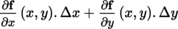 . Hence:
if D 2 f (x, y) is invertible, or equivalently if D 2 f (a, b) is invertible by continuity of D 2 f. Figure 1.1 shows that the functional relation y = u (x) might only be valid in a sufficiently small neighborhood of (a, b). If x belongs to a connected neighborhood U 0 of a, the variable y such that f (x, y) = 0 can be made arbitrarily close to b, provided that U 0 is chosen small enough. - ii) The reader may wish to find an expression for [1.16] in the finite-dimensional case using Jacobian matrices ( [DIE 93] , Volume 1, (10.2.2)); the composition of two linear mappings translates to the product of their matrices.
- iii) The statement of Theorem 1.30 no longer holds when F and G are arbitrary Fréchet spaces [SER 72] ; however, it remains valid when E is a non-complete normed vector space (see [SCH 93] , Volume 2,Theorem 3.8.5).
(III) Immersions, submersions, subimmersions, the rank theorem In the following, we assume that 0 < p ≤ ω.