Tensor Calculus on Manifolds
Abstract
Tensor calculus was the culmination of pioneering work by B. Christoffel and G. Ricci, in 1869 and 1887–1896, respectively. It reached maturity in a joint publication by Ricci-Curbastro and Levi-Cività in 1900. It is difficult to overstate its importance as a field – general relativity could not exist without it. Tensor calculus plays an essential role in every area of physics; it is also crucial for continuum mechanics and many other engineering sciences, and it, of course, lies at the heart of differential geometry. Section 4.2 of this chapter is purely algebraic (with some algebraic topology in section 4.2.6). The mathematical objects that physicists call tensors are more precisely tensor fields; they are only introduced in section 4.3. Historically, “tensors” were presented to students as exotic mathematical millipedes of the form t j 1, …, j p i 1, …, i p (or more briefly) that behave in a certain way under change of coordinates (see [4.3, 4.4]). This stemmed from the decision to only define the components of the tensor (see [4.2]). As a result, students could complete an entire course of tensor calculus without finding a satisfactory answer to the question: “But what actually is a tensor?” We will, of course, choose a different approach by defining tensor fields before attempting to study them.
Keywords
Banach spaces; Covector field; Differential form over a chain; Exterior algebra; Interior products; Metrics; Pseudo-Riemannian manifolds; Symmetric tensors; Tensor Calculus on Manifolds; Vector fields
4.1 Introduction
Tensor calculus was the culmination of pioneering work by B. Christoffel and G. Ricci, in 1869 and 1887–1896, respectively. It reached maturity in a joint publication by Ricci-Curbastro and Levi-Cività in 1900 [RIC 00]. It is difficult to overstate its importance as a field – general relativity could not exist without it. Tensor calculus plays an essential role in every area of physics; it is also crucial for continuum mechanics and many other engineering sciences, and it, of course, lies at the heart of differential geometry. Section 4.2 of this chapter is purely algebraic (with some algebraic topology in section 4.2.6). The mathematical objects that physicists call tensors are more precisely tensor fields; they are only introduced in section 4.3. Historically, “tensors” were presented to students as exotic mathematical millipedes of the form t j 1, …, j p i 1, …, i p (or more briefly) that behave in a certain way under change of coordinates (see [4.3, 4.4]). This stemmed from the decision to only define the components of the tensor (see [4.2]). As a result, students could complete an entire course of tensor calculus without finding a satisfactory answer to the question: “But what actually is a tensor?” We will, of course, choose a different approach by defining tensor fields before attempting to study them.
The fields of contravariant tensors of order 1 are just the vector fields. The fields of antisymmetric contravariant tensors of order p are called p-vector fields. The fields of covariant tensors of order 1 are the covector fields, or fields of differential forms of degree 1; the fields of antisymmetric covariant tensors of order p are the fields of differential forms of degree p, also called p-forms or p-covectors ([P1], section 3.3.8(VII)). The integral of an m-form over an m-dimensional manifold (line integral if m = 1, surface integral if m = 2, volume integral if m = 3) is a key idea that has various applications in physics (see, for example, section 5.6.4). These forms also allow us to define the orientation of a manifold (section 4.4.4). The differential forms of degree 1 go back to Euler [SAM 01]; higher-order differential forms were introduced by É. Cartan [CAR 99], who made abundant use of them [CAR 22a], whereas the differential forms “of odd type” were developed by G. de Rham [DER 84]. Differential forms are easy to define on
 or
or
 manifolds (Remark 4.33), and their exterior and interior products have properties analogous to those stated in section 4.4.3 ([KRI 97], Chapter VII, section 33).
The fields of non-degenerate symmetric covariant tensors of order 2, on the other hand, allow us to define pseudo-Riemannian manifolds, which lead to the Riemannian and Lorentz manifolds of general relativity as special cases. The notion of a Riemann space (or Riemannian manifold) is, of course, due to Riemann; they were introduced in his inaugural lecture, mentioned in section 2.1. Pseudo-Riemannian manifolds (and in particular Lorentz manifolds) are the result of a work by Minkowski, Einstein, and Grossmann ([PAU 58], Chapter II, section 7 and Chapter IV, section 50).
4.2 Tensor calculus
As a reminder, we are using the conventions outlined in section 1.2.1, especially those which relate to the representations of vectors and covectors.
4.2.1 Tensors
(I) Notion of a tensor
Let K be a field. Recall that, if E and F are K-vector spaces, the tensor product E ⊗ F is defined as the K-vector space generated by the products x
i
⊗ y
i
(x
i
∈ E, y
i
∈ E), where ⊗ E × F → E ⊗ F is a canonical bilinear mapping that is the solution of a universal problem ([P1], section 3.1.5). In particular, if (e
i
)
i ∈ I
and (f
j
)
j ∈ J
are bases of E and F, respectively, then E ⊗ F consists of the elements of the form ∑
i, j
a
ij
e
i
⊗ f
i
(a
ij
∈ K). If G is a third K-vector space, then
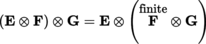 ; thus, this space can be written as E ⊗ F ⊗ G.
Let E be a finite-dimensional vector space over K, and let E
∨ be its dual.
1
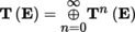
Write T
0
n
(E) = E
⊗ n
for the n-th tensor product of E, namely ⊗
i = 1
n
E
i
, where E
i
= E (i = 1, …, n), with the convention that E
⊗ 0 = K; furthermore, write T
m
0(E) = (E
∨)⊗ m
and T
q
p
(E) = T
q
0(E) ⊗ T
0
p
(E). The elements of the vector space T
q
p
(E) are called p-times contravariant and q-times covariant tensors (or tensors of type
 or (p, q))
2
; the order of any such tensor is the integer p + q. Thus, a vector of E is an element of T
0
1(E) and hence a tensor of type (1, 0), i.e. a once contravariant tensor. A linear form on E (also called a covector) is an element of T
1
0(E) and hence a tensor of type (0, 1), i.e. a once covariant tensor. The vector space T
0
n
(E) is also written as T
n
(E).
or (p, q))
2
; the order of any such tensor is the integer p + q. Thus, a vector of E is an element of T
0
1(E) and hence a tensor of type (1, 0), i.e. a once contravariant tensor. A linear form on E (also called a covector) is an element of T
1
0(E) and hence a tensor of type (0, 1), i.e. a once covariant tensor. The vector space T
0
n
(E) is also written as T
n
(E).
If E and F are finite-dimensional K-vector spaces, we know that the space E
∨ ⊗ F can be identified with
 by identifying x
∨ ⊗ y with the K-linear mapping f : x ↦ 〈x, x
∨〉 y ([P1], section 3.1.5(I)). If (e
i
∨)1 ≤ i ≤ n
is a basis of E
∨ and (f
i
)1 ≤ i ≤ m
is a basis of F, the elements of E
∨ can be represented by columns of n elements, the elements of F can be represented by rows of m elements, and so the elements of E
∨ ⊗ F can be represented by n × m matrices, like the elements of
. An element of E
∨ ⊗ F of the form x
∨ ⊗ y can be identified with an n × m matrix of rank 1. Recall that any arbitrary element of E
∨ ⊗ F is a finite sum of terms of this form.
by identifying x
∨ ⊗ y with the K-linear mapping f : x ↦ 〈x, x
∨〉 y ([P1], section 3.1.5(I)). If (e
i
∨)1 ≤ i ≤ n
is a basis of E
∨ and (f
i
)1 ≤ i ≤ m
is a basis of F, the elements of E
∨ can be represented by columns of n elements, the elements of F can be represented by rows of m elements, and so the elements of E
∨ ⊗ F can be represented by n × m matrices, like the elements of
. An element of E
∨ ⊗ F of the form x
∨ ⊗ y can be identified with an n × m matrix of rank 1. Recall that any arbitrary element of E
∨ ⊗ F is a finite sum of terms of this form.
Lemma-Definition 4.1
-
i)
The K
-vector space
 is a graduated K
-algebra ([P1], section 2.3.12) called the tensor algebra of E.
is a graduated K
-algebra ([P1], section 2.3.12) called the tensor algebra of E.
-
ii)
Let E and F be two finite-dimensional K
-vector spaces, f : E → F a linear mapping, and T (f): T (E) → T (F) the mapping uniquely determined by the condition
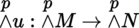
for every integer n ≥ 0 and all x 1, …, x n ∈ E. Then, T (f) is a morphism of algebras and T is a covariant functor ([P1], section 1.2.1 ) from the category of K -vector spaces into the category of graduated K -algebras (exercise).

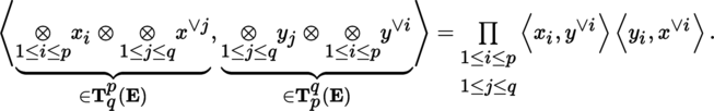
(II) Duality and index contractions The space T q p (E)∨ can be identified with T q p (E) using the relation
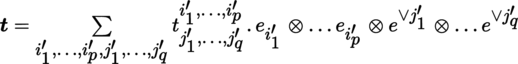
An arbitrary element t of T q p (E) can be expressed in the following form with respect to the basis (e i )1 ≤ i ≤ m of E and its dual basis (e ∨ i )1 ≤ i ≤ m :

The t j 1, …, j q i 1, …, i p are the components of the tensor t .
Write c j i for the K-linear index contraction mapping T q p (E) → T q − 1 p − 1(E), i ∈ {i 1, …, i q } and j ∈ {j 1, …, j p }, defined by 3
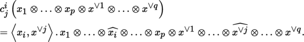
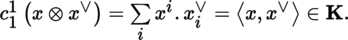
In particular, if x = ∑ i x i e i and x ∨ = ∑ i x i ∨ e i ∨, then
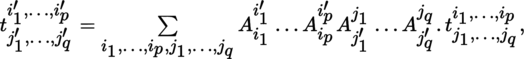
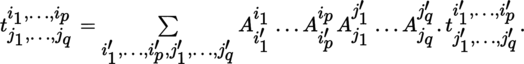
(III) Change of basis Let A = (A i j ′ ) be a change-of-basis matrix in E. Consider the tensor [4.2]. By [1.1] and [1.2], with the conventions of section 1.2.1 ( II ) and noting that K is commutative,
with
4.2.2 Symmetrie tensors and antisymmetric tensors
(I) Case of contravariant tensors
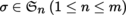
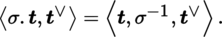
Let E be an m-dimensional K-vector space. Consider the action of the permutation group
 on space of contravariant tensors T
0
n
(E) defined by
on space of contravariant tensors T
0
n
(E) defined by

for
 .
.
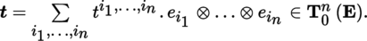
Given a basis (e i )1 ≤ i ≤ m of E, the e i 1 ⊗ … ⊗ e i n form a basis of the vector space T 0 n (E). Thus, let:
Now, define:
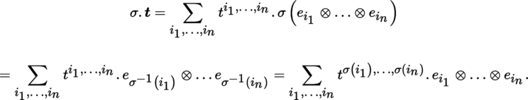
This tensor
t
is said to be symmetric, respectively antisymmetric if σ (
t
) =
t
, respectively σ
t
= ε
σ
t for every
 , where ε
σ
is the signature of the permutation σ.
, where ε
σ
is the signature of the permutation σ.
This is equivalent to saying that its coordinates satisfy:

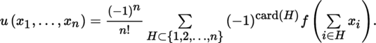
Let t ∈ T 0 n (E) The symmetrization, respectively antisymmetrization ([P1], section 3.3.8(VII)), of this tensor is defined by
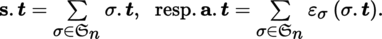
We sometimes write ([SPI 99], Volume 1, Chapter 7):

If t is already symmetric (respectively antisymmetric), then s. t = n! t (respectively a. t = n! t , so alt t = t ). Write TS n (E) ⊂ T 0 n (E) (respectively A n (E) ⊂ T 0 n (E)) for the space of symmetric (respectively antisymmetric) contravariant tensors of order n on E.
Consider the sets H = {i
1, …, i
n
} ⊂ {1, …, m}, i
1 < i
2 < … < i
n
. Then, the elements e
H
= a. (e
i
1
⊗ … ⊗ e
i
n
) form a basis of A
n
(E), and this basis has
 elements.
The space TS
n (E) can also be defined as a quotient of T
0
n
(E): consider the vector subspace
 of T
0
n
(E) generated by all the elements of the form
of T
0
n
(E) generated by all the elements of the form

for every x
i
∈ E and
. Then, TS
n
(E) can be identified with
 .
.
Lemma-Definition 4.4
-
1)
The direct sum
is called the symmetric algebra of E. -
2)
The direct sum
is a graduated ideal ([P1], section 2.3.12) of the graduated algebra T (E) ,so is a graduated K
-algebra, called the symmetric algebra of E
.
is a graduated K
-algebra, called the symmetric algebra of E
.
- 3) Proceeding in the same way as in Lemma-Definition 4.1 , we can define a covariant functor TS from the category of K -vector spaces into the category of commutative graduated K -algebras. The canonical image of (x 1, …, x n ) ∈ E n in T n (E) is written as x 1…x n .
- 4) TS (E) is isomorphic to the algebra K [X 1, …, X m ] of polynomials in m variables over K (where m := dim K (E)).

Lemma 4.6
- i) If f : E → F is a homogeneous polynomial, then the n-linear mapping u : E n → F defined by f (x) = u (x,…,x) can be chosen to be symmetric, and this choice is unique.
-
ii)
Let f : E → F be a homogeneous polynomial mapping of degree n and consider γ
n
: E
n
→ T
n
(E) : x ↦ x ⊗ … ⊗ x. There exists a unique K
-linear mapping f : T
n
(E) → F such that
 .
.
Proof
-
(i) It can be checked that
-
ii) By the universality of the tensor product ([P1], section 3.1.5(I)), there exists a unique K-linear mapping f′ from TS
n
(E) into F such that u(x
1, …, x
n
) = f
′(x
1 ⊗ … ⊗ x
n
) for all x
i
∈ E. Thus:
which gives that .
.

(II) Case of covariant tensors We saw above that T 0 n (E) can be identified with the dual of T 0 n (E) (section 4.2.1 (II)). By [4.1], it follows that:
Furthermore, T 0 n (E) can be identified with the space of n-multilinear forms on E; thus, the symmetric (respectively antisymmetric) covariant tensors can be identified with the symmetric (respectively alternating) multilinear forms on E.
4.2.3 Exterior algebra
(I) Exterior n -th power Let E be an m-dimensional K-vector space and let z p ∈ A p (E), z q ∈ A q (E) (section 4.2.2(I)). The exterior or wedge product ([P1], section 3.3.8(VII)) z p ∧ z q ∈ A p + q (E) is defined by:
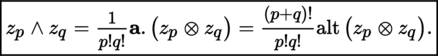
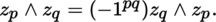
This product is associative and anticommutative, i.e.
In particular, if x, y ∈ E, then x ∧ y = a. (x ⊗ y) = x ⊗ y − y ⊗ x. If T is a twice covariant antisymmetric tensor, then

More generally, if z p i ∈ A p i (E)(i = 1, …, k), then

Applying the above to vectors z p i = x i ∈ E gives

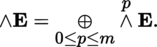
As a result of [4.9], the vector space A
n
(E) is also called the exterior n-th power of E and can be written as
 . The basis of this space associated with the basis (e
i
)1 ≤ i ≤ m
consists of the
elements:
. The basis of this space associated with the basis (e
i
)1 ≤ i ≤ m
consists of the
elements:

where the index sets H are defined as above, so that H = {i 1, …, i n } ⊂ {1, …, m}, i 1 < i 2 < … < i n . Hence,
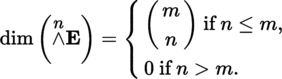
In particular,
 if n = m and
 if n > m.
Definition 4.7
The elements of
 are said to be p-vectors.
We write that
 (and so det (E) ≅ K).
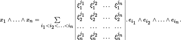
(II) Calculating an
n
-vector in a given basis
Let
 ; explicitly writing out the expression from [P1], section 3.3.8(VII) gives:
(III) Exterior algebra
Let
 and consider the direct sum
This sum has an associative K-algebra structure (for the exterior product) and is called the exterior algebra of E. The exterior algebra ∧ E is therefore clearly an anticommutative graduated K-algebra ([P1], sections 2.3.10(I) and 2.3.12), and the elements of
 are the homogeneous elements of degree p.
4.2.4 Duality in the exterior algebra
We can repeat the above for covariant tensors and covectors. This gives

with the duality bracket ([P1], section 3.3.8(VII))

and the following result:
Lemma 4.8
Let E and F be finite-dimensional K -vector spaces.
-
1)
The elements of
 can be identified with the alternating n-linear forms on E, i.e. (with the same notation as above) the n-linear forms u : E
n
→ K such that, for every permutation
and every (x
1, …, x
n
) ∈ E
n
,
can be identified with the alternating n-linear forms on E, i.e. (with the same notation as above) the n-linear forms u : E
n
→ K such that, for every permutation
and every (x
1, …, x
n
) ∈ E
n
,
where σ(u)(x 1, …, x n ) ≔ u(x σ(1), …, x σ(n)). -
2)
satisfies the following universal property (
[BOU 12]
,
Chapter III
,
section 7.4
, Proposition 7): For every alternating n-linear form u : E
n
→ F, there exists a unique K
-linear mapping
 such that
-
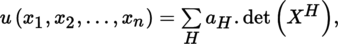
3)
In particular, suppose that dim (E) = m. Then, u : E
n
→ F is an alternating n-linear form if and only if it can be expressed in the form
where H = {j 1, …, j n } ⊂ {1, …, m}, 1 ≤ j 1 < … < j n , X H is the square matrix (η h k ) of order n satisfying η h k = ξ h jk for 1 ≤ h, k ≤ n (see section 4.2.3 (II)), and a H ∈ F.


Definition 4.9
Let E and F be finite-dimensional K
-vector spaces. Write
 for the vector space of alternating n-linear mappings (i.e. which satisfy
[4.13]
) from E
n
into F.
for the vector space of alternating n-linear mappings (i.e. which satisfy
[4.13]
) from E
n
into F.
In particular,
 is the space of p-covectors or p-forms ([P1], section 3.3.8(VII)).
Lemma-Definition 4.10
-
i)
Let u (respectively v) be an alternating p-linear (respectively q-linear) form on E
p
(respectively E
q
). The exterior product u ∧ v is defined as the antisymmetrization of the (p + q)-linear form
and v ∧ u = (–1) pq u ∧ v. Equivalently,
where Sh (p, q) is the set of permutations such that σ (1) < … < σ (p) and σ (p + 1) < … < σ (p + q).
4
such that σ (1) < … < σ (p) and σ (p + 1) < … < σ (p + q).
4
- ii) The exterior product of alternating multilinear forms is an associative operation.
-
iii)
If u
1, …, u
n
are linear forms, then u
1 ∧ … ∧ u
n
= a. ∏
i = 1
n
u
i
, or more explicitly:


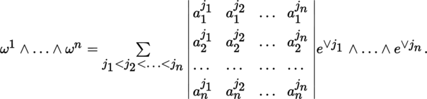
By Lemma 4.8 (2),

If ω i = ∑ j = 1 m a i j e ∨ i (i = 1, …, n), then we have the following relation, similar to [4.11]:
Remark 4.11
Some authors ( [KOB 69] , Volume I, Chapter I , p. 35) define the exterior product of an alternating linear p-form u and an alternating linear q-form v as the alternating linear (p + q) -form

We will instead write
 for this exterior product, which is equal to
 in our notation. In particular, if u
1, …, u
n
are linear forms, then
in our notation. In particular, if u
1, …, u
n
are linear forms, then
 (
[KOB 69]
, Volume I,
Chapter I
, p. 7).
(
[KOB 69]
, Volume I,
Chapter I
, p. 7).
4.2.5 Interior products
Let p, q be integers ≥ 0 and z q a contravariant tensor in T 0 q (E), where E is an m-dimensional K-vector space. The mapping v p ↦ z p ⊗ v p from T 0 q (E) into T 0 p + q (E) is K-linear. Its transpose may therefore be identified with a K-linear mapping from T 0 p + q (E ∨) into T 0 p (E), written as (with u p + q ∈ T 0 p + q (E ∨))

which is said to be the interior product of z q and u p + q . Thus, by definition:

For example, if ω is a p-covector and v 1, …,v p are vectors, then

If ψ is also a n-covector and v is a vector, this gives the “distributivity relation”:

If ω 1,…, ω p are covectors,

Remark 4.12
If we write i v (u p ):= v┘u p , then [4.15] becomes:

The interior product is an antiderivation of degree – 1 of the exterior algebra
 ([P1], section 2.3.12).
Example 4.13
- i) Suppose that q = 1, p = 0. Now, let z ∈ E = T 0 1 (E), u ∈ E ∨ = T 0 1 (E). Then, z┘u ∈ K and, for all λ ∈ K, λ. z ┘ u = 〈λ ⊗ z, u〉 = λ. 〈z, u〉, so z┘u = 〈z, u〉. The interior product is therefore a generalization of the duality bracket.
- ii)
In general, let
It can immediately be checked that - iii)
In the case of antisymmetric tensors, let
 . Define
 by the equality
for all .
.
- iv)
In particular, suppose that dim (E) = m ≥ 3, q = m – 1, p = 1, u
m
= e
∨ i
1
⊗ … ⊗ e
∨ i
m
, z
m–1 = x
1 ∧ … ∧ x
m–1, v
p
= x
0, where x
i
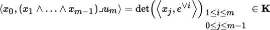
∈ E (0 ≤ i ≤ m – 1). Then:
and x 1 ∧ … ∧ x m − 1 ∈ E ∨. If E is a Euclidean space over the field of real numbers, the scalar product associates this linear form with a vector of E (this is a trivial special case of Riesz’s theorem ([P2], section 3.10.2)). This vector is again written as x 1 ∧ … ∧ x m − 1 and called the vector product of the vectors x 1 ∧ … ∧ x m − 1. The vector product does not just depend on the Euclidean structure of E , but also on its orientation (see below, section 4.4.4 ).
In the case where m = 3, the vector product of two vectors can be identified with a vector. By [4.15] , the equality [4.14] therefore implies the classical relation:


4.2.6 Tensors on Banach spaces
(I) Tensors
Let
 ,
,
 and
and
 be subcategories of the category of Banach
 -spaces ([P2], section 3.4.1
(I)) and let
-spaces ([P2], section 3.4.1
(I)) and let
 be a functor that is covariant in
 and contravariant in
 ([P1], sections 1.1.1(I) and 1.2.1).
Example 4.14
-
1)
If E is a finite-dimensional
-vector space, then μ : E
p
↦ T
0
p
(E) is a covariant functor, ν : E
q
↦ T
q
0 (E) is a contravariant functor and λ : E
p
× E
q
↦ T
q
p
(E) is a functor that is covariant in E
p
and contravariant in E
q
.
-
2)
If p = 1,
 ,
,
 , and
, and
 ,
5
we can define a functor covariant in E and contravariant in E′
q
by:
,
5
we can define a functor covariant in E and contravariant in E′
q
by:
where denotes the Banach space of continuous q-linear mappings from E′
q
into E ([P2], section 3.8.9). This functor acts as follows on morphisms: let (f, f′): (E
1, E′1) → (E
2, E′2) (where
denotes the Banach space of continuous q-linear mappings from E′
q
into E ([P2], section 3.8.9). This functor acts as follows on morphisms: let (f, f′): (E
1, E′1) → (E
2, E′2) (where
 and
and
 ); then
where f ′q = (f ′, …, f ′) (q terms). -
3)
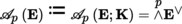
With the same conditions as (2), let Alt
q
(E′; E) be the closed subspace of
formed by the antisymmetric q-linear mappings, i.e. those which satisfy
[4.13]
for all
 and every (x′1,…, x′
q
) ∈ E′
q
, generalizing
Definition 4.9
. Write
and every (x′1,…, x′
q
) ∈ E′
q
, generalizing
Definition 4.9
. Write
 . Now, define the following functor, covariant in E and contravariant in E′:
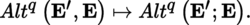
This functor acts as follows on morphisms: let (f, f ′) : (E 1, E 1 ′) → (E 2, E 2 ′) (where
and
); then
Alt q (f, f ′) : Alt q (E 2 ′; E 1) → Alt q (E 1 ′; E 2) : u ↦ f ∘ u ∘ f ′q .

For every E,
 , E′,
, E′,
 , with E = E
1 × … × E
p
, E′ = E′1 × … × E′
q
, and similarly for F and F′, set
, with E = E
1 × … × E
p
, E′ = E′1 × … × E′
q
, and similarly for F and F′, set

Definition 4.15
The functor λ is said to be a vector functor of class C
s
,
 (
section 1.2.1
(
I
)) if the following conditions are satisfied:
(
section 1.2.1
(
I
)) if the following conditions are satisfied:
-
i)
For every pair
 .
.
-
ii)
For every f ∈ Hom (E × E′; F × F′),
 .
.
-
iii)
The mapping
 is of class C
s
.
is of class C
s
.
Definition 4.16
Let B be a manifold (i.e. a Banach manifold of class C r , r ≥∞, by the conventions (C1), (C2)),
,
 , and
a vector functor of class C
r
that is covariant in the first variable and contravariant in the second. A tensor of type (p, q) is an element
, and
a vector functor of class C
r
that is covariant in the first variable and contravariant in the second. A tensor of type (p, q) is an element
 .
.
(II) Antisymmetric Continuous Multilinear Mappings
Let E, F be two Banach spaces. The space Alt
q
(E; F) of antisymmetric continuous q-linear mappings from E
q
into F is defined as in Example 4.14(3). Alt
q
(E; F) is a closed subspace of
 and hence a Banach space.
Let G, H be two other Banach spaces and Φ: F × G → H a continuous bilinear mapping; for every (y, z) ∈ F × G, write Ф(y, z) = y.z. Let u ∈ Alt p (E; F) and v ∈ Alt q (E; G). Then, the mapping

is continuous and (p + q)-linear. The statement of Lemma-Definition 4.10 remains valid in this more general context (note that the linear and multilinear mappings must be continuous), and u ∧ v ∈ Alt p + q (E; H).
The interior product v 1┘ω of v 1 ∈ E and ω ∈ Alt p (E; F) is defined by [4.14] and belongs to Alt p–1 (E; F). The relations [4.15] and [4.16] still hold, as well as Remark 4.12.
4.3 Tensor fields
Let B be a manifold and U an open subset of B. Write
 for the
-algebra of mappings of class C
r
from U into
.
for the
-algebra of mappings of class C
r
from U into
.
4.3.1 Vector fields
Definition 4.19
A vector field of class C
r
on an open subset U of B is a morphic section of T (B) over U (see
Remark 3.24
), i.e. an element of Γ(U, T (B)) (
Corollary-Definition 3.21
). The latter space is also written as
 and is a
-module.
and is a
-module.
Let (U, ξ, E) be a chart of B centered on some point a ∈ B, where E is a Banach space. The restriction to U of a vector field
 is a mapping X |
U
: U → T (B) such that π ° v = 1
U
, so
is a mapping X |
U
: U → T (B) such that π ° v = 1
U
, so

is a vector field on U. We already know that there exists an isomorphism [3.2]

4.3.2 Covector field
Definition 4.20
A covector field of class C
r
on U is a morphic section of T
∨ (B) over U, i.e. an element of Γ(U, T
∨ (B)). The latter space can alternatively be written as
 or Ω1 (U). The elements of Ω1 (U) are also known as Pfaff forms on U.
Let (U, ξ, E) be a chart of B centered on a point b ∈ B. The restriction to U of any such covector field ω isa mapping ω | U : U → T ∨ (M) satisfying π ° ω = 1 U , so
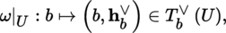
is a covector field on U. (For the finite-dimensional case, see Theorem 2.71.)
4.3.3 Tensor fields and scalar fields
(I) Tensor bundle
Let π : M → B be a vector bundle. Write T
q
p
(M) for the vector bundle of class C
r
whose fiber over an arbitrary point b ∈ B is T
q
p
(M
b
) (sections 4.2.1 and 4.2.6). This is called the bundle of p-times contravariant and q-times covariant tensors (or tensors of type (p, q)) on M. If M is of finite rank, then T
q
p
(M) = (M
∨)⊗ q
⊗ (M)⊗ p
. By convention, T
0
1(M) = M, T
1
0(M) = M
∨ (Definition 3.36) and
 . The following result is clear:
Lemma 4.21
Suppose that M is of rank n. Let (s i )1 ≤ i ≤ n be a frame of M over the open subset U of B (Lemma-Definition 3.23) and (s ∨ i )1 ≤ i ≤ n its dual frame (Lemma-Definition 3.38). Then, the n p + q tensor fields
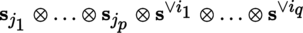
form a frame of T q p (M).
(II) Tensor product, Whitney sum and exterior product The constructions of section 3.4.4 can be extended to the tensor product and Whitney sum of an arbitrary finite number of vector bundles with the same base; in particular, we can define the tensor power M n ⊗ of a vector bundle M with base B and finite rank (section 3.4.1). We can also define the tensor field T 0 n (M) whose fibers are T 0 n (M) b (b ∈ B).
Furthermore, the same construction enables us to define the exterior power

of a vector bundle M of finite rank (with p > 0). For every sequence (s j )1 ≤ j ≤ p of sections of M on an open subset U of B, write s 1 ∧ s 2 ∧ … ∧ s p for the mapping

Remark 4.22
By convention,
 is the trivial bundle
 .
.
Consider a morphism of vector bundles u : M → N, where M and N are vector bundles with base B and finite rank. There exists a unique morphism
such that, if s 1,…, s p are arbitrary sections of M over the open set U ⊂ B, then

(III) Tensor fields Let B be a manifold, T (B) its tangent bundle and T ∨ (B) its cotangent bundle. Write T q p (B) for T q p (T(B)) if this is not ambiguous. Thus, T 0 1(B) = T(B) and T 1 0(B) = T ∨(B).
Definition 4.23
A tensor field of type (p, q) and class C
r
on an open subset U of B is a morphic section of T
q
p
(B) over U, i.e. an element of Γ(U, T
q
p
(B)). This is a mapping T : b ↦ T (b), where b ∈ U, T(b) ∈ T
q
p
(B)
b
. The space Γ(U, T
q
p
(B)) can also be written as
 (according to the notation of
Definitions 4.19
and
4.20
).
(according to the notation of
Definitions 4.19
and
4.20
).
Let (U, ξ, n) be a chart of B. Every tensor field
 can be uniquely written in the form
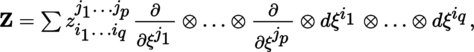
where the components z
i
1…i
q
j
1…j
p
are of class C
r
. Hence,
is a free
-module with basis

More generally, if U is an arbitrary non-empty open subset of B, then the set
is a
-module that is free whenever T (U) is trivializable, and the mapping
 is a sheaf of
 -Modules, where
is the sheaf of rings
-Modules, where
is the sheaf of rings
 (see Remark 3.34).
If B is m-dimensional, a section of class C
r
of the bundle
 of tangent p-vectors over U (section 4.2.3) is said to be a p-vector field..
(IV) Scalar fields
By Remark 4.22,
 is the set of mappings of class C
r
is the set of mappings of class C
r
 and can be identified with
.
and can be identified with
.
4.4 Differential forms
4.4.1 Differential forms of degree p
(I) Let B be a manifold. Write
 for the vector bundle of class C
r
of alternating continuous p-linear mappings from T (B) into
. The fiber of
over an arbitrary point b ∈ U is given by
for the vector bundle of class C
r
of alternating continuous p-linear mappings from T (B) into
. The fiber of
over an arbitrary point b ∈ U is given by
 (sections 4.2.1 and 4.2.6).
Definition 4.24
A differential p-form (or a differential form of degree p) on an open subset U of B is a section of class C
r
of
 on U, i.e. an element of
 (
Corollary-Definition 3.21
).
(
Corollary-Definition 3.21
).
The set Ω
p
(U) is a
-module. The mapping U → Ω
p
(U), where U is an open subset of B, is a sheaf of
-Modules. The set Ω
p
(U) is in fact just the
-module of antisymmetric p-times covariant tensor fields of class C
r
on U.
(II) Finite-dimensional case Suppose that the manifold B is locally finite-dimensional and let (U, ξ, m) be a chart of B. By Theorem 2.71, every differential form on U can be written in the form
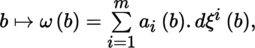
where the a
i
are m functions
 . For ω to be of class C
r
, it is necessary and sufficient for the a
i
to be of class C
r
. Every p-form α ∈ Ω
p
(U) can be uniquely written as
. For ω to be of class C
r
, it is necessary and sufficient for the a
i
to be of class C
r
. Every p-form α ∈ Ω
p
(U) can be uniquely written as

where the a
i
1, …, i
p
are of class C
r
. Hence, the differential p-forms dξ
i
1
∧ … ∧ dξ
i
p
stated above form a basis of the free
-module Ω
p
(U). The
-module Ω
p
(B) is free whenever T (B) is trivializable.
Identifying
 with the dual bundle of
, if Y1,…, Y
p
are p vector fields, then
with the dual bundle of
, if Y1,…, Y
p
are p vector fields, then

The indices h and k range from 1 to p in each determinant by [4.12].
Let
 , α (x) = f (x) dx
1 ∧ … ∧ dx
n
, and Y (x) = Σ1 ≤ i ≤ n
y
i
(x) ∂/∂ x
i
. Then, [4.14] implies that:
, α (x) = f (x) dx
1 ∧ … ∧ dx
n
, and Y (x) = Σ1 ≤ i ≤ n
y
i
(x) ∂/∂ x
i
. Then, [4.14] implies that:

(III) De Rham algebra Set
with
 (section 4.3.3
(IV)) and Ω
p
= Ω
p
(B). The notion of exterior algebra introduced in section 4.2.3 allows us to state the following result (see footnote 1(b), p. 132):
(section 4.3.3
(IV)) and Ω
p
= Ω
p
(B). The notion of exterior algebra introduced in section 4.2.3 allows us to state the following result (see footnote 1(b), p. 132):
Lemma-Definition 4.25
- 1) Let (U, ξ, m) be a chart of B. The restriction Ω | U is the exterior algebra of the free Ω0 | U -module Ω1 | U.
-
2)
The
-algebra Ω equipped with the exterior product ∧ of differential forms ([P1], section 3.3.8(VII)) is associative, graduated and anticommutative ([P1],
section 2.3.5
(IV)). The exterior product satisfies:
where # denotes the degree. We say that Ω is the de Rham algebra of differential forms on B.
4.4.2 Preimage of a differential p-form
(I) Let B, B′ be two manifolds, ω ∈ Ω p (B), and f : B′ → B a morphism of manifolds.
Lemma 4.26
There exists a uniquely determined differential p-form f ⁎ (ω) ∈ Ω p (B′) such that

for every b′ ∈ B′ and every family {v 1 ′, …, v p ′} of elements of the tangent space T b ′ (B ′).
In particular, if p = 1, then 〈f ∗(ω) b ′ , v 1 ′〉 = 〈ω (f(b ′)), T b ′ (f). v 1 ′〉 = 〈 t T b ′ (f). ω (f(b ′)), v 1〉, so
If B″ is a manifold and g : B″ → B′ is a morphism, then (exercise)

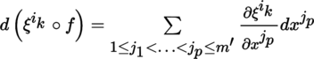
(II) If B, B′ have dimensions m, m′, respectively, (U, ξ, m) is a chart of B with ξ = (ξ i )1 ≤ i ≤ m , and ω is defined on U by [4.19], then the expression of f ⁎ (ω) on f –1 (U) is given by:
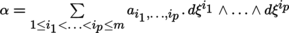
If the p-form α ∈ Ω
p
(B) can be written in the form [4.20] on U, i.e.
 , then f
⁎ (α) ∈ Ω
p
(B′) has the following expression on f
–1 (U), setting f
⁎ (α)= α ° f:
, then f
⁎ (α) ∈ Ω
p
(B′) has the following expression on f
–1 (U), setting f
⁎ (α)= α ° f:

Write ξ = f(x), x = (x 1, …, x m ′ ) Then:
and (exercise)
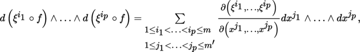
where
 is the Jacobian of (ξ
i
1
, …, ξ
i
p
) relative to (x
j
1
, …, x
j
p
) (section 1.2.2(
IV
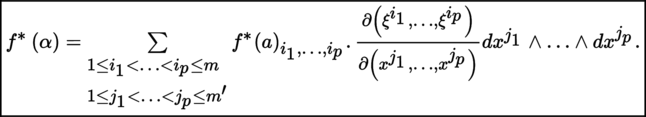
)). Hence:
is the Jacobian of (ξ
i
1
, …, ξ
i
p
) relative to (x
j
1
, …, x
j
p
) (section 1.2.2(
IV
)). Hence:
If m = m′ = p, the sum [4.20] has a single term a. dξ 1 ∧ … ∧ dξ p , and [4.23] can be restated as follows:
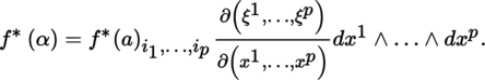
(III) Let α ∈ Ω p (B), ω ∈ Ω p (B). Then (exercise: see [DIE 93], Volume 3, (16.20.9.5)):

Remark 4.28
Definition 4.27 (which is in fact just a change of variables formula) can be extended to the case of an arbitrary covariant tensor without requiring any modifications.
6
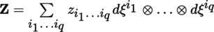
If
 is a field of p-times covariant tensors whose expression on U is given by
(see
[4.18]
) and f : B′ → B is a morphism of manifolds, then
 has the following expression on f
–1 (U):
has the following expression on f
–1 (U):
