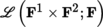
4.4.3 Differential forms taking values in a fiber bundle. List of formulas

The next section reproduces the presentation of [BOU 82a], sections 7.3 and 7.8, with slight changes to the order and a few simplifications.

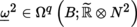
(I) Let π : N → B be a vector bundle and consider the vector bundle Alt ^p (M; N) (M = T (B)) whose fiber over an arbitrary point b ∈ B is Alt ^p (M; N) _b := Alt ^p (M _b ; N _b ) (section 4.2.6, Example 4.14(3)). If N is the trivial bundle B × F, where F is a Banach space, write Alt ^p (M; F) for Alt ^p (M; N).

Definition 4.29

A differential p-form on an open subset U of B taking values in N is a morphic section of Alt ^p (M; N), i.e. an element of Ω ^p (U; N):=Γ (U, Alt ^p (M; N)).

Clearly, for any open subset U of B, Ω ^p (U ; N) is a C r U -module and the mapping U → Ω ^p (U ; N) is a sheaf of C r -Modules.

Remark 4.30

1. i)  In the above, we can replace M by an arbitrary vector bundle of class C ^r and base B. We can alternatively write Ω ^p (U ; N):=Γ (U, Alt ^p (M; N)), where the fiber bundle M is implicit on the left-hand side.
2. ii)  With p = 0, Ω⁰ (U; N) is the set of sections of class C ^r of the form G : U → N : b ↦ (b, n _b ) that are liftings of 1 _U (thus, n _b ∈ N _b and π ° G = 1 _U ).
3. iii)  If N is the trivial bundle B × F, where F is a Banach space, then Ω ^p (U ; N) is written as Ω ^p (U ; F).

(II) Exterior product Let π ⁱ : N ⁱ → B (i = 1,2) and π : N → B be three vector bundles of class C ^r and Φ a mapping from N ¹ × _Β N ² into N. Suppose that, for every b ₀ ∈ B, there exist an open neighborhood U of b ₀ in B and vector charts t ⁱ = (U ⁱ , φ ⁱ , F ⁱ ) of π ⁱ (i = 1, 2) and t = (U, φ, F) of π, together with a mapping λ of class C ^r in ℒ F 1 × F 2 F , satisfying the following condition: for every b ∈ U and all (x ¹, x ²) ∈ F ¹ × F ² (with the notation of Definition 3.22(i), Condition (V)),

t b ∘ λ b x 1 x 2 = Φ t b 1 x 1 t b 2 x 2 .

Definition 4.31

The mapping Φ defined above is said to be a coupling of the fiber product N ¹ × _Β N ² ( section 2.3.9 ) in N.

Suppose that one such coupling is given and let M be a fiber bundle with base B and of class C ^r . For every b ∈ B, there is a continuous bilinear mapping

Φ b : Alt p M N 1 b × Alt q M N 2 b → Alt p + q M N b .

The collection of these continuous bilinear mappings determines a coupling

u : Alt p M N 1 × Alt q M N 2 → Alt p + q M N .

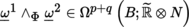
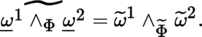
Given sections ω ¹, ω ² of Alt ^p (M; N ¹) and Alt ^q (M; N ²) on U, the section u (ω ¹, ω ²) of Alt ^p + q (M; N) on U is written as ω ¹ ∧_Φ ω ² (see Remark 4.18).

Definition 4.32

We say that ω ¹ ∧_Φ ω ² is the exterior product of ω ¹ and ω ². This exterior product is written as ω ¹ ∧ ω ² whenever the coupling Φ is implicitly clear.

If the s _i (i = 1, …, p + q) are morphic sections of M on U, then:

ω 1 ∧ Φ ω 2 s 1 … s p + q = ∑ σ ε σ Φ ω 1 s σ 1 … s σ p ω 2 ( s σ p + 1 … s σ p + q ) ,

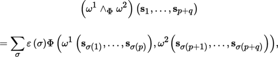
where the sum ranges over permutations of {1, …, p + q} such that σ (1) < … < σ (p) and σ (p + 1) < … < σ (p + q) (see Lemma-Definition 4.10(i)).

(III) De Rham algebra: generalization An algebra bundle of base B is a vector bundle A of base B equipped with a coupling from A × _Β A into A. In the following, the fibers A _b (b ∈ B) are assumed to be associative and commutative algebras with neutral element e _b ([P1], section 2.3.10(I)). Let π : M → B be a vector bundle with base B (e.g. T (B)). Write Ω ^p (U; A) (where U is an open subset of B) for the C r U -module formed by the morphic sections of Alt ^p (M; A) on U.

The exterior product allows the direct sum Ω(U; A) = ⊕ _p ≥ 0Ω ^p (U; A) to be equipped with the structure of an associative, anticommutative and graduated algebra, again called the de Rham algebra (section 4.4.1(III)).

If ω = ω ₁ ∧ … ∧ ω _p , where ω _i ∈ Ω¹ (U; A), and s _i is a morphic section of M on U (i = 1,…, p), then (see [4.21]):

ω s 1 … s p = det ω i s j .

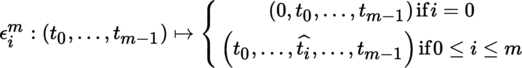
(IV) Interior product Let p ≥ 1. There exists a coupling i from M × _Β Alt ^p (M; A) into Alt ^p–1 (M; A) whose restriction to each fiber is the interior product (Remark 4.12). If s is a section of M on the open subset U of B and ω ∈ Ω ^p (U; A), write i (s) ω for the section i (s, ω) of Alt ^p–1 (M; A) on U. Then, for every b ∈ U,

i s ω b = s b ┘ ω b .

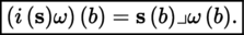
We say that i (s) ω is the interior product of s and ω. From this definition and the formulas listed in section 4.2.5, we can deduce the following relations (where the s _j are sections of M):

i s ω ⏟ degree p s 1 … s p − 1 = ω s s 1 … s p − 1 , i s ∘ i s = 0 , i s ω ⏟ degree 1 = ω s , i s . ω ⏟ degree p ∧ ω ′ = i s ω ∧ ω ′ + − 1 p ω ∧ i s ω ′ , i s ω 1 ∧ … ∧ ω p ⏟ forms of degree 1 = ∑ i = 1 p − 1 i + 1 ω i s ω 1 ∧ … ∧ ω i ^ ∧ … ∧ ω p .

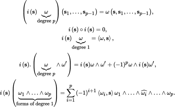
The interior product is an antiderivation of degree – 1 of the de Rham algebra ([P1], section 2.3.12).

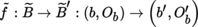
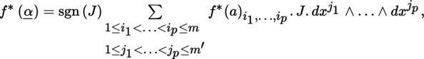
(V) Preimage Let f : B′ → B be a morphism of manifolds and ω ∈ Ω ^p (B; N). Let f ^⁎ (N) be the preimage of N under f (section 3.4.6). There exists a uniquely determined differential p-form f ^⁎ (ω) such that [4.22] holds (mutatis mutandis). For every family of vector fields X′₁, …, X′ _p of class C ^r on B′, the mapping

f ∗ ω X 1 ′ … X p ′ : b ′ ↦ f ∗ ω b ′ X 1 ′ b ′ … X p ′ b ′

is a lifting of f into N (Definition 3.6, section 3.3.1).

In particular, a differential 0-form G on B′ taking values in N is in fact just a lifting of class C ^r of f into N, i.e. a mapping (of class C ^r ) G : B′ → N such that G (b′) ∈ N _{f (b′)} for all b′ ∈ B′.

(VI) Vector-valued differential forms The fiber bundle Ω ^p (B; N) is trivial if and only if N is trivial (section 3.4.1, Example 3.26(a)), or in other words N = B × F, where F is a Banach space (exercise). If so, the fibers N _b can be identified with F. We write Alt ^p (M; F) for Alt ^p (M; N), Ω ^p (B; F) for Ω ^p (B; N), and we say that ω is a vector-valued differential p-form taking values in F. In particular, if K = ℝ , N = T (B), and F = ℂ , then ω is a complex differential p-form on the real manifold B.

The usual fiber bundle Alt p T B K can also be written as Alt p T B K B = Alt p T B B × K , and

Ω p B = Γ Alt p T B B × K .

   [4.25]

Remark 4.33

The space of differential p-forms on an ℱ N or SN manifold can be defined using [4.25] ( [KRI 97] , Chapter VII , section 33).

4.4.4 Orientation

For the rest of this chapter, excluding section 4.5.1, every manifold is a locally finite-dimensional differential manifold and F always denotes a Banach space.

(I) Orientation of a vector space Let E be a real m-dimensional vector space. We know that dim ∧ m E = 1 (section 4.2.3(I)), so det E ≔ ∧ m E is the union of two closed half-lines on the real axis with opposite directions and origin 0. These half-lines are written as O and –O. The set {O, –O} formed by these half-lines is written as Or (E).

(II) Orientation of a real manifold Let Β be a manifold and M = T (B). Write

Or M = ∪ • b ∈ B Or M b .

Lemma 4.34

Let π ˜ : Or M → B be the mapping defined by π ˜ b O = b for every b ∈ Β. There exists a unique topological space structure on Or _M for which the following two conditions are satisfied:

1. i)  π ˜ is continuous.
2. ii)  If s is a continuous, everywhere non-zero section of the vector bundle det (M) (whose fibers are the det (M _b ), b ∈ Β, with the notation of (I), implying that s(b) ∈  det (M _b ) = O(b) ∪ (− O((b))) on an open subset U of Β and s (b) ∈ O (s (b)) for every b ∈ U, then the mapping B → Or _M : b ↦ O (s (b)) is continuous (exercise).

Suppose that the topological space Or _M is equipped with the manifold structure determined by taking the preimage under π ˜ of the manifold structure of Β (Remark 2.44), and consider the fibration π ˜ : Or M → B . The multiplicative group {± 1} acts simply transitively (and hence freely) ([P1], section 2.2.8(II)) on Or _M by O ↦ –O. The manifold of orbits of this action is Or _M \{± 1} ≅ B.

Corollary-Definition 4.35

1. 1)  The fibration π : Or _M → Β is a principal bundle with structural group {± 1}. This principal bundle B ˜ is a covering of Β with fiber type {± 1} ( section 3.3.3 ), namely a covering of two leaves.
2. 2)  The principal bundle B ˜ is said to be the orientation covering. An orientation of Β is a continuous section O : b ↦ (b, O _b ) of B ˜ O b ∈ ± 1 . If any such section exists, the pair (B, O) is said to be an oriented manifold. The orientations O and –O are said to be opposite.
3. 3)  A manifold B is said to be orientable if there exists an orientation on B.
4. 4)  A pure m-dimensional manifold B is orientable if and only if one of the following equivalent conditions is satisfied:
   1. i)  The orientation covering B ˜ is the trivial bundle B × {± 1}.
   2. ii)  There exists a continuous differential m-form v ₀ such that v ₀ (b) ≠ 0 for every b ∈ B; if so, v ₀ is of class C ^∞, i.e. v ₀ ∈ Ω ^m (B). Since dim (Ω ^m (B)) _b = 1, the sign of v ₀ (b) must be constant on B, and v ₀ determines an orientation O : b ↦ (b, sgn (v ₀ (b))) of B (where sgn denotes the sign).
   3. iii)  There exists an atlas of B whose charts (U _i , φ _i , n _i ) satisfy the property that, if U _i  ∩ U _j  ≠ ∅ (which implies n _i = n _j ), then

      ∂ φ i 1 … φ i n i ∂ φ j 1 … φ j n j > 0

      

      
      on U _i  ∩ U _j .
5. 5)  Hence, if B is a pure orientable m-dimensional manifold, then the relation ∼ on Ω ^m (B) defined by v ∼ v′ if sgn (v (b)) = sgn (v′ (b)) (where b is an arbitrary point of B) is an equivalence relation. The orientation O : b ↦ (b, sgn (v (b))) is the equivalence class of v, written as v ¯ .

Proof

(4): See [DIE 93], Volume 3, (16.21.1), (16.21.16). (5): exercise.

Corollary 4.36

1. 1)  Let B be a manifold and b some point of B. By Corollary-Definition 4.35 (4), there exists an open neighborhood U of b in B that is orientable.
2. 2)  A manifold B is orientable if and only if each of its connected components is orientable.
3. 3)  Let (B, O) be a pure m-dimensional oriented manifold and v ₀ ∈ O. Every differential m-form ω ∈ Ω ^m (B) can be uniquely written in the form ω = f.v ₀, where f : B → ℝ is of class C ^∞. Given b ∈ B, write ω b > < ¯ 0 if f b > < ¯ 0 .
4. 4)  Let (B, O) be a pure m-dimensional oriented manifold. If ω ∈ Ω ^m (B; F), there exists a unique mapping f : B → F of class C ^∞ satisfying ω = f.v ₀ (exercise).

Definition 4.37

Let (B, O) be an oriented manifold and v ₀ ∈ O. A sequence (Z ₁,…, Z _m ) of vector fields is said to be positive or direct (respectively negative or retrograde) if, for every b ∈ B,

v 0 b Z 1 b ∧ … ∧ Z m b > 0 resp . < 0 .

Example 4.38

1. i)  The space ℝ m is orientable and the canonical m-form dx ¹ ∧ … ∧ dx ^m (where x ⁱ is the i-th coordinate function in the canonical basis) defines its canonical orientation.
2. ii)  More generally, the underlying manifold of a finite-dimensional real Lie group G is always orientable. Indeed, suppose that G is m-dimensional, and let z ^∨ be an m-covector such that z _e ^∨ ≠ 0 (where e is the neutral element); then the differential m-form g ↦ γ (g) z ^∨ (of class C ^ω ), where γ is left translation ( section 2.4.1 ( I )), is non-zero at every point.
3. iii)  Every simply connected manifold and every parallelizable manifold ( Definition 3.28 ) is orientable ( [NAR 73] , Corollary 2.7.6; [LEE 02] , Proposition 10.5).
4. iv)  In particular, the sphere S n (see footnote 2, p. 98) is orientable.
5. v)  Every finite product of orientable manifolds is orientable. If B ₁, B ₂ are two manifolds with orientations O ₁, O ₂ respectively, the mapping (b ₁, b ₂) ↦ O _b1 O _b2 is an orientation of B ₁ × B ₂ written as O ₁ ⊗ O ₂.
6. vi)  Let B bean oriented manifold with orientation O. Let U be a submanifold of B. The mapping O | _U is an orientation of U. Hence, every submanifold of an orientable manifold is orientable.
7. vii)  It can be shown that any finite-dimensional pure differential manifold B ₀ underlying a holomorphic manifold B is orientable ( [DIE 93] , Volume 3, (16.21.13)).
8. viii)  The Möbius strip (see Figure 3.2 in section 3.3.1 and footnote 3, p. 98) and the Klein bottle (see footnote 6, p. 70) are not orientable. The Möbius strip is a striking example of a non-orientable manifold: any reader who wishes to experiment with the concept of orientation can make a Möbius strip by gluing together the two ends of a strip of paper with a half-twist. Now, draw a pencil line along the middle of the strip – the line will almost magically reach “the other side” of the strip from the starting point.

Let (B, O) be an oriented manifold. If we write this oriented manifold as B ↷ , we can write B ↶ or − B ↷ for the manifold equipped with the opposite orientation.

4.4.5 Integral of a differential form of maximal degree

(I) Volume integrals in ℝ m

Lemma 4.39

Let U, U′ be open subsets of ℝ m and u : U → U′ a diffeomorphism. For every x ∈ U, let J = det ∂ u ∂ x be the Jacobian of u ( section 1.2.2 ( IV )). Let λ U ⊗ m  ≔ λ ⊗ m  | U and λ U ′ ⊗ m be the Radon measures induced on U and U′, respectively, by the Lebesgue measure on ℝ m ([P2], section 4.1.5(I)). Then, the image of | J |. λ U ⊗ m under u is λ U ′ ⊗ m ([P2], section 4.1.5(II)); in other words, for every function f ∈ K U ′ , where K U ′ denotes the space (of type ℒ s ℱ ) of compactly supported continuous functions from U′ into ℝ ([P2], section 4.1.4(IV)), we have the following change of variable formula, by [4.24] :

∫ U ′ f x ′ . d λ ⊗ m x ′ = ∫ U f u x . J x . d λ ⊗ m x .

This relation still holds if we replace f ∈ K U ′ by a λ ^⊗ m -integrable mapping f : U′ ↦ F ([P2], section 4.1.2).

Example 4.40

Let U and U′ be two open intervals on the real line and u a diffeomorphism from U onto U′. Let f be a continuous function on U taking values in the Banach space F . The function t ↦ u (t) is monotone, so u . t has constant sign ε on U, and:

∫ U f t . dt = ∫ U ′ f u t . ε . u . t . dt = ∫ U ′ f u t . u . t . dt .

Example 4.41

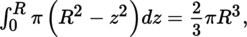
Let us calculate the volume V of a sphere of radius R.

1. 1)  Cartesian coordinates. Pick the center of the sphere as the origin, and begin by calculating the volume of the hemisphere z ≥ 0. We can use the Fubini-Tonelli theorem ([P2], section 4.1.3(III)) to do this by cutting the hemisphere into “slices” of infinitely small thickness dz. Each slice is a cylinder with a circular cross-section of radius R 2 − z 2 and thickness dz. The volume of the hemisphere is therefore given by

   ∫ 0 R π R 2 − z 2 dz = 2 3 π R 3 ,

   

   
   which gives us the classical formula V = 4 3 π R 3 .
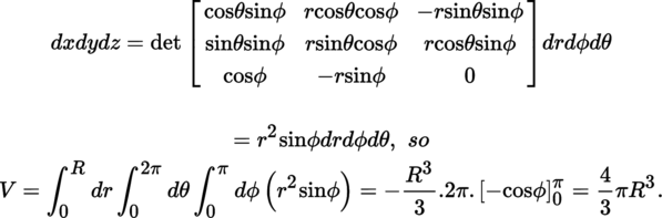
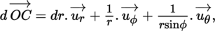
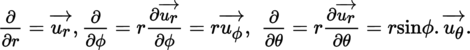
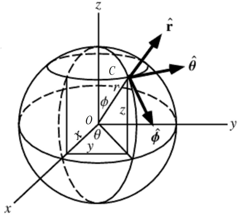
2. 2)  Spherical coordinates. In mathematics, the radial, azimuthal, and zenithal coordinates {r, ϕ, θ} are defined as shown in Figure 4.1 , with r ≥ 0, 0 ≤ θ ≤ 2π, and 0 ≤ ϕ ≤ π (in physics, the symbols θ and ϕ are often swapped). These coordinates satisfy the relations:

   x = r cos θ sin ϕ , y = r sin θ sin ϕ , z = r cos ϕ .

      [4.26]

   
   Hence, by Lemma 4.39 ,

   dxdydz = det cos θ sin ϕ r cos θ cos ϕ − r sin θ sin ϕ sin θ sin ϕ r sin θ cos ϕ r cos θ sin ϕ cos ϕ − r sin ϕ 0 drdϕdθ = r 2 sin ϕdrdϕdθ , so V = ∫ 0 R dr ∫ 0 2 π dθ ∫ 0 π dϕ r 2 sin ϕ = − R 3 3 .2 π . − cos ϕ 0 π = 4 3 π R 3 .

      [4.27]

   
   Let C be the point with Cartesian coordinates (x, y, z). Then, dC → = e 1 → dx + e 2 → dy + e 3 → dz , where e 1 → , e 2 → , e 3 → are the vectors of the canonical basis. In spherical coordinates, write u r → , u ϕ → , u θ → for the unit vector along the direction of OC → , the unit vector tangent to the meridian in the direction of increasing ϕ, and the unit vector parallel to C in the direction of increasing θ, respectively. Then , OC → = r u r → , OC → = u r → . dr + r ∂ u r → ∂ ϕ . dϕ + r ∂ u r → ∂ θ . dθ = ∂ ∂ r dr + ∂ ∂ φ dφ + ∂ ∂ θ dθ with u r → = cos θ sin ϕ . e 1 → + sin θ sin ϕ . e 2 → + cos ϕ . e 3 → , so

   d OC → = dr . u r → + 1 r . u ϕ → + 1 r sin ϕ . u θ → ,

      [4.28]

   
   

   ∂ ∂ r = u r → , ∂ ∂ ϕ = r ∂ u r → ∂ ϕ = r u ϕ → , ∂ ∂ θ = r ∂ u r → ∂ θ = r sin ϕ . u θ → .

      [4.29]

   
   The orthonormal frame u r → u ϕ → u θ → is positively oriented, since the determinant [4.27] is positive.
3. 3)  Calculation based on the radial coordinate, the longitude, and the latitude. The coordinates are now (r, φ, λ) (see Example 2.12 , section 2.2.1 ( II )). In radians, the latitude φ and the longitude λ may now be expressed as a function of the zenith φ and the azimuth θ by φ = π 2 − ϕ and λ = θ – π. Starting from the expressions [2.1] , an analogous calculation gives dxdydz = r ² cos φdrdφdλ, and

   V = ∫ 0 R dr ∫ − π π dλ ∫ − π / 2 π / 2 dφ r 2 cos φ = R 3 3 .2 π . sin φ − π / 2 π / 2 = 4 3 π R 3 .

   

Figure 4.1 Spherical coordinates

(II) Lebesgue measures

Corollary-Definition 4.42

Let B be a pure m-dimensional manifold. There exists a positive Radon measure μ on B ([P2], section 4.1.5(V)) with the following properties:

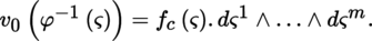
1. i)  For every chart c = (U, φ, m) of Β, the image under φ ([P2], section 4.1.5(II)) of the induced measure μ _U is of the form f _c . λ _φ(U) ^⊗ m , where f _c is a function of class C ^∞ that does not vanish on φ (U).
2. ii)  In other words, for every function g ∈ K U ,

   ∫ U g b dμ b = ∫ φ U g ς f c ς d λ ⊗ m ς .

   

3. iii)  Any Radon measure μ with the property (i) is said to be Lebesgue on B. Any two Lebesgue measures μ, μ′ on B are equivalent in the sense that each is absolutely continuous with respect to the other ([P2], section 4.1.6(III)) and each has a density function ofclass C ^∞ with respect to the other.

(III) Integral of a form of maximal degree over an m -dimensional oriented manifold Let B ↷ be a pure oriented manifold of dimension m ≥ 0 and let ω be a differential m-form taking values in a Banach space F. our next task is to give meaning to the quantity

∫ B ↷ ω .

By Corollary-Definition 4.35(5), there exists a differential m-form v ₀ ∈ Ω ^m (B) that belongs to the orientation of B ↷ . Let c = (U, φ, m) be a chart of B such that the open set U is connected. For every point ζ = (ζ¹,…, ζ ^m ) ∈ φ (U), we can write (with the same notation as above):

v 0 φ − 1 ς = f c ς . d ς 1 ∧ … ∧ d ς m .

Since U is connected, f _c is of class C ^∞ and has constant sign in φ (U). Let μ _{v 0, U} , U be the positive Radon measure on U defined by

μ v 0 , U = φ − 1 f c . λ φ U ⊗ m .

If we proceed in the same way for another arbitrary chart c′ = (U′, φ′, m) of B, where U′ is also connected, we obtain a measure μ v 0, U ′ that is positive on U′. It is easy to show ([DIE 93], Volume 3, (16.24.1)) that, if U ∩ U ′ ≠ ∅, the restrictions of μ v 0, U and μ v 0, U ′ ′ to U ∩ U ′ are equal. The positive measures μ v 0, U (as U ranges over the set of connected open subsets of B, which form a covering of B) are, therefore, the restrictions to U of a unique positive Radon measure μ v 0 (which is Lebesgue) defined on B. With the same hypotheses and notation as Corollary 4.36(4):

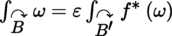
Corollary-Definition 4.43

The differential m-form ω is said to be integrable (over B ↷ )if f is μ _{v 0} -integrable. If so, define:

∫ B ↷ ω ≔ ∫ B ↷ f . d μ v 0 .

This quantity only depends on the orientation of B ↷ and not on the particular choice of v ₀ made to specify this orientation.

Let ω ∈ Ω ^m (B; F) be an integrable differential m-form on B ↷ taking values in F. With the notation introduced at the end of section 4.4.4 (II):

∫ − B ↷ ω = ∫ B ↷ ω .

If g ∈ K B and ω ∈ Ω ^m (B; F), then g.ω is a continuous m-form and g ↦ ∫ B ↷ g . ω is a Radon measure [ω] taking values in F ([P2], section 4.1.5(VIII)). 7

Definition 4.44

The Radon measure [ω] defined on B is called the volume form on B ↷ determined by the differential m-form ω.

The above leads to the following result ([DIE 93], Volume 3, (16.24.2)):

Corollary 4.45

If ω ∈ Ω ^m (B) belongs to the orientation of B ↷ , then the volume form

ω : K B → ℝ : g ↦ ∫ B ↷ g . ω

is a positive Lebesgue measure on B ↷ . Conversely, every positive Lebesgue measure on B ↷ is of the form [ω], ω ∈ Ω ^m (B).

(IV) Orientation of a morphism

Definition 4.46

Let B, B′ be locally finite-dimensional manifolds and f : B → B′ a morphism. An orientation of f is a morphism f ˜ : B ˜ → B ˜ ′ : b O b → b ′ O b ′ that makes the diagram

B ˜ → f ˜ B ′ ˜ ↓ π ↓ π ′ B → f B ′

commute and which is compatible with the group action {± 1}. In other words, 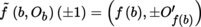f ˜ b O b ± 1 = f b ± O f b ′ . We write that f ˜ = f ε , ε ∈ {–1, 1}.

Corollary-Definition 4.47

1. 1)  Let B, B′ be orientable manifolds, f : B′ → B a diffeomorphism, and f ˜ = f ε an orientation of f. Let O be an orientation of B and write B ↷ = B O . There exists a unique orientation O′ on B′ such that, setting B ↷ = B ′ O ′ , every differential form ω ∈ Ω ^m (B; F) satisfies

   ∫ B ↷ ω = ε ∫ B ′ ↷ f ∗ ω

      [4.30]

   
   (exercise). The orientation O′ is said to be associated with O by f ˜ .
2. 2)  Conversely, let B ↷ , B ′ ↷ be two oriented manifolds and f : B′ → B a diffeomorphism. If the relation [4.30] is satisfied for every differential form ω ∈ Ω ^m (B; F) and ε = + 1, we say that f preserves orientations, or that f reverses orientations if ε = –1. The pair f ˜ = f ε is an orientation of f, where f is viewed as a diffeomorphism from B′ onto B (and B and B′ are the orientable manifolds underlying B ↷ and B ′ ↷ , respectively).

(V) Canonical orientation of the orientation covering Let B be a manifold and . π ˜ : B ˜ → B the orientation covering (Corollary-Definition 4.35(1)). Let b ˜ = b O b ∈ B ˜ . The projection . π ˜ : B ˜ ↠ B is the linear mapping b ˜ ↦ b . Its tangent linear mapping T b ˜ π ˜ : T b ˜ B ˜ → T b B is an isomorphism, so π ˜ is a local diffeomorphism (Theorem 2.61(2)), i.e. a diffeomorphism from an open subset U of b ˜ onto an open subset V of b. We can choose U and V to be orientable (Corollary 4.36(1)); thus, there exists an orientation O : b ˜ ↦ O b ′ of V taking the value O _b at the point b. We have π ˜ − 1 b = b O b b − O b . Let ω ∈ O, ω ˜ = π ˜ ∗ ω , and O ˜ = ω ˜ ¯ (see Corollary-Definition 4.35(5)); then b ˜ ↦ O ˜ b ˜ is an orientation of B ([DIE 93], Volume 3, (16.21.6)), which gives us the following result:

Theorem 4.48

The manifold B ˜ is orientable.

Remark 4.49

1. (1)  The space . π ˜ : B ˜ ↠ B is a covering of two leaves. It therefore has a canonical involution 8 ι : B ˜ → B ˜ that permutes these leaves over each point b ∈ B. If O ˜ is an orientation of B ˜ , then the orientation of B ˜ associated with ι ( Corollary-Definition 4.47 ) is − O ˜ . Therefore, both O ˜ and − O ˜ are orientations of B ˜ ; nevertheless, we say that O ˜ is the canonical orientation. This ambiguity is irrelevant in practice because O ˜ is unique up to permutation of the two leaves of B ˜ .
2. 2)  Conversely, if π ¯ : M → B is an oriented covering of class C ^∞ with two leaves and its canonical involution associates a given orientation of M with the opposite orientation, then π ¯ : M → B is isomorphic to π ˜ : B ˜ → B ( [LEB 82] , Chapter I , section 5.C, Theorem 2).

4.4.6 Differential forms of odd type

(I) Definition The fiber bundle ℝ ˜ ≔ B ˜ × ± 1 associated with B ˜ of fiber type ℝ (section 3.5.5) is called the bundle of scalars of odd type. Let N be a vector bundle of base B. A differential p-form ω ¯ ∈ Ω p B ℝ ˜ ⊗ N is said to be a differential p-form of odd type on B taking values in N. Let . π ˜ : B ˜ ↠ B be the projection. There exists a bijection

• ˜ : ω ¯ ↦ ∼ ω ˜

   [4.31]

between the differential p-forms of odd type on B taking values in N and the differential p-forms on B ˜ taking values in π ˜ ∗ N such that ω ˜ − O = − ω ˜ O for every orientation O ∈ B ˜ .

Remark 4.50

1. a)  When B is equipped with an orientation O, the bijection

   Ω p B N → Ω p B ℝ ˜ ⊗ N : ω ↦ ω ¯ ≔ O ⊗ ω

      [4.32]

   
   allows us to identify the usual differential p-forms ω on B ↷ with the differential p-forms of odd type ω ¯ on B ↷ . Thus, in most cases, we do not need to talk about differential forms of odd type on an oriented manifold. However, the concept of differential p-form of odd type becomes crucial on manifolds without an orientation (especially when these manifolds are non-orientable). Whenever we talk about p-forms on these manifolds, we will always be referring to differential p-forms of odd type.
2. b)  We also say that an ordinary differential form (belonging to Ω ^p (B; N))is even and that a differential form of odd type (belonging to Ω p B ℝ ˜ ⊗ N )is odd ( [DER 84] , Chapter II ). This more simple terminology is adopted below.

If N is the trivial bundle B × F, we write Ω p B ℝ ˜ ⊗ F for the space Ω p B ℝ ˜ ⊗ N , and we say that the odd p-form ω ¯ ∈ Ω p B ℝ ˜ ⊗ F takes values in F.

(II) Preimage Let f : B → B′ be a morphism, f ˜ : B ˜ → B ˜ ′ an orientation of f (Definition 4.46), and ω ¯ ∈ Ω p B ℝ ˜ ⊗ N .

Definition 4.51

The preimage f ∗ ω ¯ is the odd differential form in Ω p B ℝ ˜ ⊗ f ∗ N uniquely determined by the following property ( [BOU 82a] , 10.4.2): let ω ˜ (respectively f ∗ ω ¯ ˜ ) be the differential p-form on B ˜ ′ (respectively B ˜ ) associated with ω ¯ (respectively f ∗ ω ¯ ) by the bijection • ˜ from [4.31] ; then the following relation holds:

f ˜ ∗ ω ˜ = f ∗ ω ¯ ˜ .

(III) Exterior and interior products Given three fiber bundles N ¹, N ², N with the same base B, a coupling Φ from N ¹ × _B N ² into N (Definition 4.31), and two odd differential forms ω ¯ 1 ∈ Ω p B ℝ ˜ ⊗ N 1 , ω ¯ 2 ∈ Ω q B ℝ ˜ ⊗ N 2 , we can define the exterior product ω ¯ 1 ∧ Φ ω ¯ 2 ∈ Ω p + q B ℝ ˜ ⊗ N in the same way as in Definition 4.32. The coupling Φ uniquely determines a coupling Φ ˜ from N ˜ 1 × B N ˜ 2 into N ˜ , and (exercise)

ω ¯ 1 ∧ Φ ω ¯ 2 ˜ = ω ˜ 1 ∧ Φ ˜ ω ˜ 2 .

If ω ¹ and ω ² are differential forms of same parity (respectively of opposite parity) (Remark 4.50(b)), then ω ¹ ∧_Φ ω ² is an even (respectively odd) differential form.

The formulas satisfied by the exterior product and the interior product (section 4.4.3 (II),(IV)) also hold for odd differential forms.

(IV) Change of variable In practical settings, an odd differential p-form α ¯ can be expressed locally in the form [4.20]. Even differential p-forms satisfy the change-of-variable formula [4.23], whereas the corresponding formula satisfied by odd differential p-forms is as follows:

f ∗ α ¯ = sgn J ∑ 1 ≤ i 1 < … < i p ≤ m 1 ≤ j 1 < … < j p ≤ m ′ f ∗ a i 1 , … , i p . J . dx j 1 ∧ … ∧ dx j p ,

   [4.33]

where J = ∂ ξ 1 … ξ n ∂ x 1 … x n ([DER 84], Chapter II, section 5).

(V) Measure defined by an odd m -form Let B be an m-dimensional Hausdorff pure manifold, ω ¯ ∈ Ω m B ℝ ˜ ⊗ F , and O ^m the canonical orientation of ℝ m (Example 4.38(i)). Let c =(U, φ, m) be a chart of B.

Lemma 4.52

There exists a unique mapping f _c : φ (U) → F so that

ω ¯ U = φ ∗ O m ⊗ f c . dx 1 ∧ … ∧ dx m .

We say that ω ¯ is locally integrable if f _c is locally λ _U ^⊗ m -integrable. If so, there exists a unique Radon measure α ω ¯ taking values in F that satisfies the following property: for every chart c = (U, φ, m) of B, φ α ω ¯ = f c . λ U ⊗ m .

Definition 4.53

The Radon measure α ω ¯ is said to be defined by the odd differential m-form ω ¯ and is also written as ω ¯ .

Remark 4.54

Suppose that F = ℝ ; let B ↷ be an oriented m-dimensional manifold with orientation O. Let ω ∈ Ω ^m (B), ω ¯ = O ⊗ ω (see [4.32] ). Unlike the Radon measure [ω] from Definition 4.44 , the Radon measure ω ¯ from Definition 4.53 is not necessarily positive. We have the relation ω = ω ¯ ([P2], section 4.1.5(VI)). In a certain sense, the notion of an odd differential form transfers the orientation of the manifold over to the form (see Example 4.55 ).

Example 4.55

Let Β be the cube 0 < ξ ⁱ < 1 in ℝ 3 ; this is an open subset of ℝ 3 and hence a submanifold ( section 2.3.3 ). Write B ↷ for the manifold B equipped with the orientation induced by the canonical orientation of ℝ 3 ( Example 4.38 (vi)).

1. a)  The “algebraic volume” of B ( [SCH 93] , Volume IV, Chapter VI , Remark 12) is (see Corollary 4.45 )

   V = ∫ B ↷ ω = ∫ B ω ,

      [4.34]

   
   with ω := dξ¹ ∧ dξ² ∧ dξ³ ∈ Ω³ (B) (ordinary differential 3-form) and [ω] = λ _B ^⊗ 3.
   Let φ : (x ¹, x ², x ³) ↦ (ξ¹, ξ², ξ³), where ξ² = x ¹, ξ¹ = x ², x ³ = ξ³. By [4.24] ,

   φ ∗ ω = dx 1 ∧ dx 2 ∧ dx 3 ⇒ φ ∗ ω = ω = λ B ⊗ 3 .

   

   
   However, φ reverses the orientation of B ( Corollary-Definition 4.47 (2)), so φ ∗ B ↷ = − B ↷ , and performing the change of variable φ transforms V into

   φ ∗ V ≔ ∫ − B ↷ ω = − ∫ B ↷ ω = − ∫ B ω = − V .

   

2. b)  Now consider the odd differential 3-form ω ¯ ≔ d ξ 1 ∧ d ξ 2 ∧ d ξ 3 ∈ Ω 3 B ℝ ˜ . This time, we have:

   V = ∫ B ω ¯ .

   

   
   By [4.33] , φ ∗ ω ¯ = − ω ¯ , so ⁹

   φ ∗ V = ∫ B φ ∗ ω ¯ = ∫ B − ω ¯ = − V .

      [4.35]

Remark 4.56

Since the differential forms ω and ω ¯ from Example 4.55 have the same expression (dξ¹ ∧ dξ² ∧ dξ³), they are often written in the same way (even though the first belongs to Ω³ (B) and the second belongs to Ω 3 B ℝ ˜ ; strictly speaking, they are distinct objects).

4.4.7 Integration of a differential form over a chain

(I) Integration over an odd simplex Recall that the standard m-simplex Δ ^m in ℝ m is defined by

Δ m = ∑ i = 0 m t i v i : t i ≥ 0 ∑ 0 ≤ i ≤ m t i = 1 ,

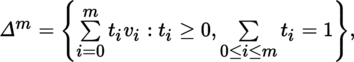
where v ₀ = 0and { v ₁, …, v _m } is the canonical basis of ℝ m ([P1], section 3.3.8(V)). Let U be an open neighborhood of Δ in ℝ m , F a Banach space, and ω ∈ Ω ^m (U; F) an even m-form (Remark 4.32(b)). Since the space ℝ m is equipped with an orientation O, we can calculate ∫ U ↷ χ Δ m . ω , where χΔ ^m is the characteristic function of Δ ^m and U ↷ is equipped with the orientation induced by O.

Definition 4.57

Let B be a pure, metrizable, m-dimensional manifold. An odd m-simplex in B is a triple τ ¯ = Δ m σ O , where Δ ^m is the standard m-simplex in ℝ m , U is an open neighborhood of Δ ^m , σ is a mapping of class C ^∞ from U into B and O is an orientation of ℝ m .

In algebraic topology, B is a topological space, σ is only assumed to be continuous, O is the canonical orientation of ℝ m and τ ¯ can be identified with σ. In differential geometry, where σ is of class C ^∞, we sometimes specify that τ ¯ is a smooth simplex.

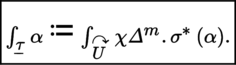
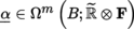
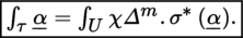
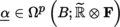
Let α ∈ Ω ^m (B; F) be an even m-form. The preimage σ ^⁎ (α) is an even m-form in Ω ^m (U; F). Set:

∫ τ ¯ α ≔ ∫ U ↷ χ Δ m . σ ∗ α .

(II) Integration over an even simplex Let Δ ^m , U, F, σ, B be as defined above.

Definition 4.58

An even m-simplex in B is a pair τ = Δ m σ ˜ , where σ ˜ ≔ σ ε is an orientation of a mapping σ of class C ^∞ from U into B ( Definition 4.46 ).

Consider an odd differential m-form α ¯ ∈ Ω m B ℝ ˜ ⊗ F . Its preimage σ ∗ α ¯ is another odd differential m-form (Definition 4.51). Set:

∫ τ α ¯ = ∫ U χ Δ m . σ ∗ α ¯ .

   [4.36]

Remark 4.59

If α ∈ Ω p B F (respectively α ¯ ∈ Ω p B ℝ ˜ ⊗ F ), where p < m, then ∫ τ ↷ α = 0 (respectively ∫ τ α ¯ = 0 ), since we are integrating over a set of measure zero. If α ∈ Ω B F is an even non-homogeneous differential form Σ_{0 ≤ p ≤ m} α _p , then ∫ _τ α = ∫ _τ α _m , and an analogous result holds when integrating an odd non-homogeneous differential form over an even simplex.

(III) Integration over a chain There are two cases to consider:

1. i) integration of an odd form over an even chain;
2. ii) integration of an even form over an odd chain.

The remarks up to and including part (IV) discuss the first case (i). The second case (ii) is similar and is left to the reader.

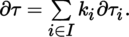
Let {τ _i : i ∈ I} be a set of even m-simplexes in the metrizable, pure, m-dimensional manifold B. The free group with this set as a basis is the set S _m (B) of linear combinations with integer coefficients

τ = ∑ i ∈ I k i . τ i ,

   [4.37]

where all but finitely many of the k _i are zero ([P1], section 3.3.8(VI)). It is useful to consider the real vector space S m B ⊗ ℤ ℝ formed by allowing these sums to have real coefficients; any such sum is called a chain of simplexes (ibid.).

Example 4.60

A closed, convex polyhedron 10 in ℝ m is a finite intersection of closed half-spaces. Any closed polyhedron is a finite union of convex closed polyhedra ( [BOU 82a] , 11.3.1). A closed polyhedron is a chain of simplexes (see [P1], section 3.3.8(VI) for a demonstration of how to express a square as the sum of two simplexes), so a chain of closed polyhedra is a chain of simplexes.

In the following, every chain is a chain of simplexes. If α ¯ ∈ Ω m B ℝ ˜ ⊗ F , set

∫ τ α ¯ ≔ ∑ i ∈ I k i . ∫ τ i α ¯ .

   [4.38]

This definition still makes sense in the obvious way if the chain τ = ∑ _i ∈ I k _i τ _i . is allowed to be infinite (i.e. the sum is allowed to include infinitely many non-zero terms) and the set supp α ¯ ∩ τ is compact.

(IV) Change of variable Let B′ be another metrizable pure m-dimensional manifold, suppose that f : B → B′ is a morphism, and let f ˜ = f ε ′ be an orientation of f .If τ = Δ m π ˜ is an even simplex in B, then f τ ≔ Δ m f ˜ ∘ π ˜ is an even simplex in B′. From [4.38], we can deduce the definition of f (τ) when τ is an even chain in B. By [4.36],

∫ τ α ¯ = ∫ f τ f ∗ α ¯ .

(V) Boundary of a chain The i-th face of the standard m-simplex Δ ^m in ℝ m is ϵ _i ^m  : Δ ^m − 1 ↦ Δ ^m , where ([P1], section 3.3.8(VI))

ϵ i m : t 0 … t m − 1 ↦ 0 t 0 … t m − 1 if i = 0 t 0 … t i ^ … t m − 1 if 0 ≤ i ≤ m

Given an m-simplex τ = Δ m σ ˜ , its boundary ∂ τ is defined as follows for m ≥ 1 :

∂ τ ≔ ∑ i = 0 m − 1 i σ ∘ ϵ i m .

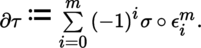
If τ ∈ S m B ⊗ ℤ ℝ is the chain defined by [4.37], where the τ _i are m-simplexes, write:

∂ τ = ∑ i ∈ I k i ∂ τ i .

   [4.39]

The boundary ∂(τ) is a chain with the same parity as the chain τ. If these chains are odd (which will be assumed henceforth), the orientation of ∂ (τ) above is said to be induced by the orientation of τ. Consider, for example, the triangle Δ² in the plane, equipped with its canonical orientation, and write v ₀, v ₁, v ₂ for its vertices; then ([P1], section 3.3.8(V)) ∂ Δ 2 = v 0 v 1 v 2 ^ + v 0 ^ v 1 v 2 + − v 0 v 1 ^ v 2 : see Figure 4.2

Figure 4.2 Δ² and its boundary ∂ Δ²

.

Remark 4.61

Consider one of the segments [v _i , v _j ]. The interior ]v _i , v _j [ of this segment is a submanifold of the plane (Oxy). Suppose that this submanifold is oriented as shown in Figure 4.2 , writing ξ for this orientation and η for some point of ]v _i , v _j [. The canonical orientation O of the plane (Oxy) is positive in the direction (Oz) and contains each of the elements v ∧ u, where v is a vector pointing strictly outward at η for Δ² (with the obvious meaning in this context) and u belongs to ξ. The orientation ξ is induced by O.

Lemma 4.62

Let ∂ _m : Δ ^m → Δ ^m–1. Then, ∂ _m–1 ° ∂ _m = 0.

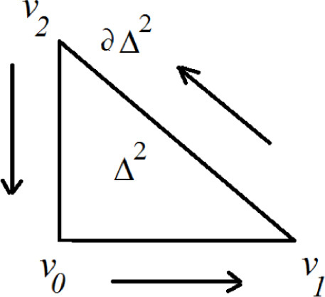
Proof

We have:

∂ m v 0 … v m = ∑ i = 0 m − 1 i v 0 … v i ^ … v m , ∂ m − 1 v 0 … v i ^ … v m = ∑ j = 0 i − 1 − 1 j v 0 … v j ^ … v i ^ … v m + ∑ k = i + 1 m − 1 k − 1 v 0 … v j ^ … v i ^ … v m ,

and ∂ _m − 1 ∘ ∂ _m [v ₀, …, v _m ] = 0.

(VI) Orientation of a boundary Our next task is to specify the notion of the boundary of an odd chain, as well as the orientation of this boundary. This is straightforward if we proceed as described in Remark 4.61. Let τ be an odd chain in an m-dimensional manifold B (m ≥ 2) and write Fr (τ) for its frontier. The latter is the union of a submanifold ∂ τ of dimension m – 1, called the regular boundary (or simply the boundary) of τ (in the example from Remark 4.61, this is the union of the open segments ]v _i , v _j [), and a set of points contained in a submanifold of dimension m – 2 (the endpoints of the segments, in the example).

Let b ∈ ∂ τ and suppose that ξ is an orientation of T _b (∂ τ). Write ι ˜ b ξ for the orientation of T _b (B) containing each of the vectors v ∧ u, where v is a vector pointing strictly outward from τ at b and u is a non-zero element of ∧ m − 1 T b ∂ τ that belongs to the orientation ξ. The mapping ι ˜ b is a bijection from Or (T _x (∂ τ) onto Or (B) and the ι ˜ b b ∈ ∂ τ determine a morphism ι ˜ : ∂ τ ˜ → B ˜ that is an orientation of the canonical injection i : ∂ τ ↪ B (section 4.4.5(IV)).

Definition 4.63

If O is an orientation of B, the orientation of ∂ τ associated with O by ι ˜ ( Corollary-Definition 4.47 ) is said to be induced by O.

4.5 Pseudo-Riemannian manifolds

4.5.1 Metric

Let B be a Banach manifold of class C ^r (r ≥ ∞) and g :(X, Y) ↦ g (X, Y) = 〈X | Y〉 a twice covariant Hermitian tensor field of class C ^r . For every b ∈ B,

g b ∈ T 2 0 T b B = ℒ 2 ( T b B , T b B K .

Consider the condition (M) and the weaker condition (WM) stated below:

( M ) For every b ∈ B and all X b ∈ T b ( B ) , the mapping g ( Y b , . ) b : T b ( B ) → K : X b ↦ Y b X b b

is an anti-linear bijection from T _b (B) onto T _b ^∨ (B) ([P2], section 3.10.1(I)).

( WM ) For every b ∈ B and all X b ∈ T b ( B ) , the mapping g ( Y b , . ) b : T b ( B ) → K : X b ↦ Y b X b b

is non-degenerate (i.e. if g (Y _b , X _b ) _b = 0 for all X _b ∈ T _b (B), then Y _b = 0).

If B is locally finite-dimensional (which is typically the case in practice), the conditions (M) and (WM) are equivalent.

Definition 4.64

Let B be a manifold equipped with a twice covariant Hermitian tensor field g of class C ^r . If g satisfies (M) (respectively (WM)), the manifold B is said to be strongly (respectively weakly) pseudo-Riemannian. 11 The field g is called the metric or the fundamental tensor field of the manifold. This manifold is said to be strongly (respectively weakly) Riemannian if the Hermitian form g (b) is also positive definite for every b ∈ B.

Suppose now that K = ℝ and let B be a pure m-dimensional manifold.

Definition 4.65

A frame (h _α)_{1 ≤ α ≤ m} of T (B) (Definition 3.23) is said to be orthonormal for the metric g if

h α b h β b b = η b α β . δ α β

   [4.40]

for every b ∈ B, where η _b , (α, β) ∈ {1, –1}. We say that g (b) has signature (p _b , m – p _b ) if, for every β ∈ {1,…, m}, Card {α ∈ {1, …, m} : sgn (η _b (α, β)) = 1} = p _b .

If B is connected, the signature of g is constant. Let (U, ξ, m) be a chart; we can express g locally (over U) by

g = ∑ i , j = 1 m g ij . d ξ i ⊗ d ξ j ,

   [4.41]

where the square matrix G (b) = (g _ij (b)) is real, symmetric, and nowhere singular. Any such chart is said to be a system of normal pseudo-Riemannian coordinates at the point b ∈ B if the system of tangent vectors ∂ ∂ ξ 1 b … ∂ ∂ ξ m b is orthonormal for the real symmetric form 〈.|.〉 _b .

The real manifold B is Riemannian if the symmetric form g (b) has signature (m, 0) at every point; if m ≥ 2 and the signature is (1, m – 1) or (m – 1, 1) at every point, then the manifold B is said to be Lorentzian (the Lorentzian manifold of dimension 4 is encountered in general relativity; we will call it the Einstein manifold).

4.5.2 Pseudo-Riemannian volume element

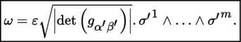
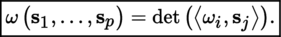
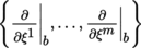
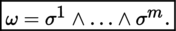
Let {σ ^α :1 ≤ α ≤ m} be the dual coframe of the orthonormal frame (h _α )_{1 ≤ α ≤ m} (Lemma-Definition 3.38). The pseudo-Riemannian volume element for which the frame (h _α )_{1 ≤ α ≤ m} is positively oriented is (Definition 4.37 and section 4.4.5(III)):

ω = σ 1 ∧ … ∧ σ m .

Let (h β′) be another, arbitrary frame. Let (σ β′) be its dual, and suppose that A = (A α ′ α ) is the inverse change-of-basis matrix satisfying h α ′  = ∑ α h α ′ A α ′ α (see [1.2], section 1.2.1( II )). Then, by [4.40], using the fact that g is bilinear,

g α ′ β ′ = ∑ α , β A α ′ α A β ′ β g h α h β ′ = ∑ α A α ′ α A β ′ α η ,

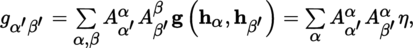
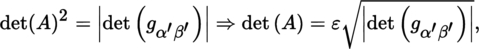
where g _{α ^′ β ^′}  = g(h _α , h _{β ^′} ). Writing (g _{α ^′ β ^′} ) for the matrix with entries g _{α ^′ β ^′} ,we therefore have det(g _{α ^′ β ^′} ) =  det (A)² η, which implies that

det A 2 = det g α ′ β ′ ⇒ det A = ε det g α ′ β ′ ,

where ε =+1if the frame (h β′) is positively oriented and ε = – 1 otherwise. Moreover, σ α  = ∑ α ′ A α ′ α σ α ′ , so

ω = ∑ σ ∈ S m ε σ A σ 1 1 … A σ m m σ ′ 1 ∧ … ∧ σ ′ m = det A . σ ′ 1 ∧ … ∧ σ ′ m

(see [P1], section 2.3.11(V)) and hence

ω = ε det g α ′ β ′ . σ ′ 1 ∧ … ∧ σ ′ m .

   [4.42]

---

1 (a) Since E is finite-dimensional, its dual ([P2], section 3.6.1) coincides with its algebraic dual ([P1], section 3.1.2). (b) Up to and including section 4.2.5, we can replace K by a commutative ring A and the finite-dimensional K-vector spaces by finitely generated A-modules ([P1], section 2.3.1 (II)).

² This convention has been adopted by various authors, including [DIE 93, BoU 12, BIS 68], but is not universal. For example, the opposite convention is found in ([SPI 99], Vol. 1, p. 123), where p-times contravariant and q-times covariant tensors are said to be of type q p

³ The notation . ^ indicates that the symbol (.) should be omitted.

⁴ The notation Sh is short for shuffle.

⁵ Recall that the dual of E is written as E ^∨ rather than E′, which for us denotes an arbitrary Banach space in B 1 .

⁶ There is no equivalent definition for contravariant and mixed tensors, except for vector fields (see below, Definition 5.14).

⁷ The cited reference only considers measures taking values the dual E ^∨ of a finite-dimensional space E. However, extending this concept to measures taking values in an arbitrary Banach space F is entirely straightforward (see, for example, [SCH 93], Volume III, Definition 5.4.6).

⁸ An involution is a bijection that coincides with its inverse bijection.

⁹ In [4.34] and [4.35], we have avoided writing ∫ _U d[ω] and ∫ U d ω ˇ for the integrals relative to the measures [ω] and ω ˇ respectively, differing from the convention adopted in ([P2], section 4.1.5(II)), as this would inevitably result in confusion with the exterior differential.

¹⁰ See the Wikipedia article Polyhedron.

¹¹ In the case where B is locally finite-dimensional (the only case considered below), the adverbs strongly and weakly can be omitted.