Proof
The Banach space F can be identified with F 1 × F 2, and since D i (a) is an isomorphism from E onto F 1, E can be identified with F 1. By translation, we may assume that a = 0. Let

We have φ (x, 0) = i (x) and Dφ(0, 0) = D i(0) + (0, 1 F 2 ). Since D i (0) is an isomorphism from F 1 onto F 1 × 0, Dφ (0, 0) is an isomorphism from F 1 × F 2 onto F 1 × F 2. By Theorem 1.29, φ is a local diffeomorphism of class C p that admits an inverse diffeomorphism r of class C p . Hence, there exists an open neighborhood U of a in F 1 such that, for all x ∈ U, r (i (x)) = x.
Recall that every closed subspace of a Hilbert space E splits in E ([P2], section 3.10.2(II), Theorem 3.147(2)). Corollary 1.33 shows that any immersion of class C p admits a local retraction r of class C p . Immersions are therefore local sections (see [P1], section 1.1.1 (III)).
Corollary-Definition 1.33
-
1)
Let E, F be Banach spaces, A a non-empty open subset of E, a ∈ A and s : A → F a mapping of class C
p
such that D
s (a) is surjective with a kernel E
2 that splits in E (i.e.
 ). Then, there exist an open neighborhood U ⊂ A of a and a diffeomorphism ψ of class C
p
). Then, there exist an open neighborhood U ⊂ A of a and a diffeomorphism ψ of class C
p
where V 1 × V 2 ⊂ A (V i ⊂ E i ) is an open neighborhood of a in E, such that s ∘ ψ is the first projection V 1 × V 2 ↠ V 1 . - 2) The mapping s defined above is called a submersion of class C p .
Proof
By translation, we may assume that a = (a 1, a 2) = (0, 0). Thus, D 1 s (0, 0) is an isomorphism from E 1 onto F that allows these two Banach spaces to be identified. Let

Then, Dφ (0) is represented by the matrix
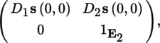
which is an automorphism of E 1 × E 2. By Theorem 1.29, there exist a neighborhood U ⊂ A of 0 in E 1 × E 2 and a diffeomorphism φ : U → V 1 × V 2 of class C p with inverse diffeomorphism ψ : V 1 × V 2 → U of class C p . For all y 1 ∈ V 1, we have f (ψ (y 1, x 2)) = y 1.
([P2], section 3.2.2 (IV), Theorem 3.5(3)) implies the following result:
Corollary-Definition 1.34
-
1)
Let E, F be Banach spaces, A a non-empty open subset of E, a ∈ A, and f : A → F a mapping of class C
p
. The following conditions are equivalent:
- i) There exist an open neighborhood U of a, U ⊂ A, a Banach space G , a submersion s of U into G of class C p and an immersion i of G into F of class C p such that f | U = i ∘ s.
-
ii)
There exist an open neighborhood U ⊂ A of a, a diffeomorphism
 of class C
p
, where U′ is an open subset of E, a mapping
of class C
p
, where U′ is an open subset of E, a mapping
 and a diffeomorphism
 of class C
p
, where V is an open neighborhood of f (a) in F and V′ = Φ (U′) is an open subset of F, such that
of class C
p
, where V is an open neighborhood of f (a) in F and V′ = Φ (U′) is an open subset of F, such that
and the kernel and image of Φ split.
- 2) The mapping f defined above is called a subimmersion of class C p .

The composition of two immersions is an immersion, the composition of two submersions is a submersion and, given a subimmersion f, an immersion i, and a submersion s, the mapping i ∘ f ∘ s is a subimmersion (exercise). However, the composition of two subimmersions is not always a subimmersion ([DIE 93], Volume 3, section 16.8, Problem 1(b)).
Theorem 1.35
(rank) Let E, F be Banach spaces, A some non-empty open subset of E and f : A → F a mapping ofclass C 1.
- i) If f is a subimmersion, there exists an open neighborhood U ⊂ A of a in E such that rk x (f) = rk a (f) for all x ∈ U.
- ii) Conversely, if there exists an open neighborhood U ⊂ A of a in E such that rk x (f) = rk a (f) for all x ∈ U and if the spaces E, F are finite-dimensional, then f is a subimmersion at the point a.
-
iii)
Write rk
x
(f) = +∞ if rk
x
(f) is not finite. The mapping x ↦ rk
x
(f) from A into the discrete subspace
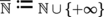 of the extended real line
 is lower semi-continuous ([P2],
section 2.3.3
(III)) in A.
is lower semi-continuous ([P2],
section 2.3.3
(III)) in A.
Proof
(i): By [1.18], rk
x
(f)= rk (Φ) for all x ∈ U. (ii): See [DIE 93], Volume 1, (10.3). (iii): If r = rk
a
(f) < +∞, we may assume that
 and extract a square submatrix M
x
that has rank r at x = a from the Jacobian matrix of f at the point x. The determinant Δx of this submatrix is therefore non-zero for x = a. But the mapping x ↦ Δ
x
is continuous, so there exists a neighborhood U of a in which Δ
x
≠ 0, and so rk
x
(f) ≥ r. If rk
a
(f) = +∞, then, for all
and extract a square submatrix M
x
that has rank r at x = a from the Jacobian matrix of f at the point x. The determinant Δx of this submatrix is therefore non-zero for x = a. But the mapping x ↦ Δ
x
is continuous, so there exists a neighborhood U of a in which Δ
x
≠ 0, and so rk
x
(f) ≥ r. If rk
a
(f) = +∞, then, for all
 , there exist vectors e
1, …, e
r
∈ E such that the vectors D
f (a).e
1, …, D
f (a).e
r
generate a subspace of F of dimension r. Arguing by contradiction, we deduce that there exists a neighborhood U of a in which rk
x
(f) = +∞.
, there exist vectors e
1, …, e
r
∈ E such that the vectors D
f (a).e
1, …, D
f (a).e
r
generate a subspace of F of dimension r. Arguing by contradiction, we deduce that there exists a neighborhood U of a in which rk
x
(f) = +∞.
1.3 Other approaches to differential calculus
1.3.1 Lagrange variations and Gateaux differentials
In this section,
 .
.
(I) Affine spaces
Given a vector space E, an affine space
 attached to the space E is a homogeneous space of the additive group E ([P1], section 2.2.8(II)) such that the (transitive) action of E on
is faithful, i.e. such that the neutral element 0 is the only element of E that fixes every element of
. The action of x ∈ E on
attached to the space E is a homogeneous space of the additive group E ([P1], section 2.2.8(II)) such that the (transitive) action of E on
is faithful, i.e. such that the neutral element 0 is the only element of E that fixes every element of
. The action of x ∈ E on
 is written as P + x. We say that E is the space of translations of
, its elements are the translations of
and, if dim (E) < ∞, this quantity is called the dimension of
. Given some origin O chosen from
, the elements of
are all of the form O + x (x ∈ E).
is written as P + x. We say that E is the space of translations of
, its elements are the translations of
and, if dim (E) < ∞, this quantity is called the dimension of
. Given some origin O chosen from
, the elements of
are all of the form O + x (x ∈ E).
Remark 1.36
The mapping O + x ↦ x is a bijection from
onto E that allows these two sets to be identified.
If Q = P + x, we write
 (the bipoint of origin P and endpoint Q)
7
. If E is a locally convex space, the sets O + U = {O + x : x ∈ U}, where the U are the open sets of E, define a topology on
. When equipped with this topology,
is called a locally convex affine space. Every point of such a space admits a fundamental system of convex neighborhoods. We can similarly define the concepts of affine topological space, affine normed space, affine pre-Hilbert space, etc.
(the bipoint of origin P and endpoint Q)
7
. If E is a locally convex space, the sets O + U = {O + x : x ∈ U}, where the U are the open sets of E, define a topology on
. When equipped with this topology,
is called a locally convex affine space. Every point of such a space admits a fundamental system of convex neighborhoods. We can similarly define the concepts of affine topological space, affine normed space, affine pre-Hilbert space, etc.
(II) Lagrange variations
Let
 be a locally convex affine space, F a locally convex space, A some non-empty subset of
, a some point of A and f : A → F a mapping.
be a locally convex affine space, F a locally convex space, A some non-empty subset of
, a some point of A and f : A → F a mapping.
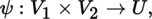
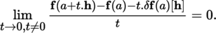
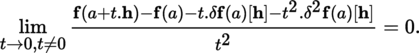
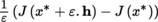
We say that f admits a Lagrange first variation δ f (a): E → F : h ↦ δ f (a) [h] at the point a if, for all h ∈ E,
If this condition is satisfied, we say that f admits a Lagrange second variation δ 2 f (a): E → F if
The Lagrange variation of order n, δ n f (a) : E n → F : h ↦ δ n f (a) [h], is defined inductively in the same way.
(III) Gateaux differentiability It is easy to show using the generalized Goursat theorem (section 1.2.5 (III)) that, if E and F are complex locally convex spaces and f admits a Lagrange first variation at the point a, then δ f (a) is linear ([HIL 57], Theorem 26.3.2). In general, we have the following result:
Lemma 1.37
If f admits a Lagrange first variation δ
f (a), then the mapping δ
f (a): E → F is homogeneous, i.e. δ
f (a) [λ.h] = λ.δ
f (a) [h] for all
 and all h ∈ E (exercise).
The set
 of G-differentiable mappings at the point a is an affine space. A G-differentiable mapping is not necessarily continuous. If E is a normed vector space and f is differentiable at the point a, then it is also G-differentiable at this point and D
f (a) = D
G
f (a) (exercise). On product spaces, we may define the Gateaux partial differential D
1
G
f (a
1, a
2) in the first variable and, similarly, in the second variable, etc. In the conditions of Theorem 1.9, where
of G-differentiable mappings at the point a is an affine space. A G-differentiable mapping is not necessarily continuous. If E is a normed vector space and f is differentiable at the point a, then it is also G-differentiable at this point and D
f (a) = D
G
f (a) (exercise). On product spaces, we may define the Gateaux partial differential D
1
G
f (a
1, a
2) in the first variable and, similarly, in the second variable, etc. In the conditions of Theorem 1.9, where
 and
and
 (and B denotes an open subset of F containing f (A)), we have
 and (instead of [1.5])

(exercise *: see [ALE 87] section 2.2.2).
Let
be a normed affine space, F a locally convex space, A a non-empty open subset of
, [a, a + h] a segment contained in A and f : A → F a G-differentiable mapping. Then, the mean value theorem (Theorem 1.13(i)) remains valid (exercise
*: see [ALE 87], section 2.2.3) in the form

where |.|γ is a continuous semi-norm on F. The claims (ii) and (iii) of this theorem also hold after making analogous adjustments. From this, we deduce the following result:
Corollary 1.39
Let E be a normed vector space, A some non-empty open subset of E, F a locally convex space and f : E → F a mapping that is G-differentiable in A. If
 is continuous, then f is differentiable in A.
Proof
Let ε > 0 and γ ∈ Γ, where (|.|)γ ∈ Γis the family of semi-norms which defines the topology of F. There exists δ = δ (ε, γ) > 0 such that, ∀ x ∈ A,

Let h ∈ E be such that | h | < δ. The relation [1.8] with the modifications stated above implies that | f (a + h) − f (a) − D G f (a).h |γ ≤ ε | h |.
Thus, we do not need to distinguish between Fréchet and Gateaux differentiation when talking about mappings of class C p (p > 0).
1.3.2 Calculus of variations: elementary concepts
In this section,
.
(I) Euler condition
Let
be a locally convex affine space, A some non-empty open subset of
, a some point of A and
 a mapping that admits a Lagrange first variation δJ (a) at the point a.
Proof
By translating the origin, we may assume that a = 0. Similarly, we can assume that J has a minimum at 0 for clarity. We will argue by contradiction. Assume that δJ (0) ≠ 0. There exists h ∈ A such that β := δJ (0) [h] ≠ 0. By Lemma 1.37, we may assume without loss of generality that β < 0 (replacing h by − h if necessary). There exists a function φ defined in some open neighborhood of 0 in
 satisfying lim
t → 0 φ (t) = 0 and J (t.h) = J (0) + t.β + t.φ(t). Pick t > 0 sufficiently small that β + φ (t) < 0. Then, J (t.h) < J (0), contradiction.
satisfying lim
t → 0 φ (t) = 0 and J (t.h) = J (0) + t.β + t.φ(t). Pick t > 0 sufficiently small that β + φ (t) < 0. Then, J (t.h) < J (0), contradiction.
(II) Euler-Lagrange equation
The Euler–Lagrange equation is essentially the Euler condition applied to calculus of variations. A full treatment would require another volume
8
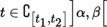
; we will content ourselves with briefly mentioning the simplest part, which is sufficient for our purposes. Let E be a Banach space and suppose that
 , t
1 < t
2.
, t
1 < t
2.
Proof
We will argue by contradiction from the assumption that f (t
0) ≠ 0. There must therefore exist z ∈ E such that 〈f (t
0), z〉 > 0. Since f is continuous, there exists an interval [α, β] ⊂ [t
1, t
2] containing t
0 such that α < β and 〈f (t), z〉 > 0 for all t ∈ [α, β]. There exists a function
 of class C
1 that is zero in
of class C
1 that is zero in
 and which satisfies φ (t) > 0 for t ∈ ]α, β[; for example, φ (t) = (t − α)2 (β − t)2 if t ∈ ]α, β[ and φ (t) = 0 if
 . Therefore, setting h (t) = φ (t).z, we have ∫
t
1
t
2
〈f(t), h(t)〉dt > 0, contradiction.
. Therefore, setting h (t) = φ (t).z, we have ∫
t
1
t
2
〈f(t), h(t)〉dt > 0, contradiction.
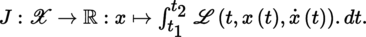
Let Ω1, Ω2 be non-empty open subsets of E and let

be a mapping (known as the Lagrangian in mechanics) of class C
1 with partial differential
 . Let x
1, x
2 ∈ Ω1 and write
. Let x
1, x
2 ∈ Ω1 and write
 for the set of mappings x : [t
1, t
2] → Ω1 of class C
1 satisfying x (t
1) = x
1, x (t
2) = x
2 whose derivatives
for the set of mappings x : [t
1, t
2] → Ω1 of class C
1 satisfying x (t
1) = x
1, x (t
2) = x
2 whose derivatives
 take values in Ω2. The set
is an open subset of the normed affine space O + X, where X is equipped with the norm
take values in Ω2. The set
is an open subset of the normed affine space O + X, where X is equipped with the norm
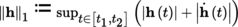 ; X is a Banach space whose elements satisfy the condition h (t
1) = h (t
2) = 0 (exercise). Let
; X is a Banach space whose elements satisfy the condition h (t
1) = h (t
2) = 0 (exercise). Let
Theorem 1.44
Let
 be a mapping of class C
2
9
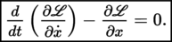
. The relation δJ (x
*) = 0 holds, i.e. x
* is an extreme point of J, if and only if x
* is a solution of the Euler–Lagrange equation:
be a mapping of class C
2
9
. The relation δJ (x
*) = 0 holds, i.e. x
* is an extreme point of J, if and only if x
* is a solution of the Euler–Lagrange equation:
Proof
Let h ∈ X. If ε > 0 is sufficiently small, then
 . Thus,

Let
 . The mapping (ε, t) ↦ f (ε, t) has a partial derivative
 whose absolute value is upper bounded by a function g : t ↦ g (t) that is integrable in [t
1, t
2]. Therefore, as ε ↦ 0,
whose absolute value is upper bounded by a function g : t ↦ g (t) that is integrable in [t
1, t
2]. Therefore, as ε ↦ 0,
 converges ([P2], section 4.1.2(II), Theorem 4.11) to
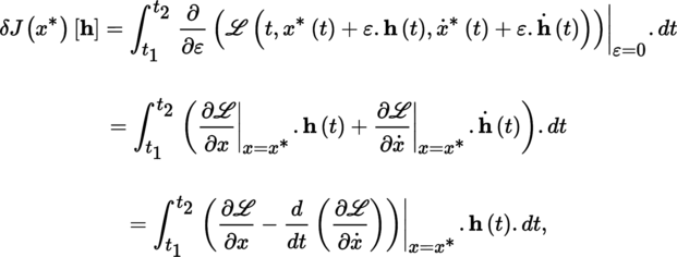
which gives the desired result by Lemma 1.43.
The Lagrangian
 is said to be regular at x = x
* if
is said to be regular at x = x
* if
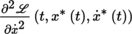 is invertible in
 for every t ∈ [t
1, t
2].
for every t ∈ [t
1, t
2].
Corollary 1.45
(Hilbert) If
is a solution of the Euler–Lagrange equation
[1.21]
and the Lagrangian is regular at x = x
*, then x
* is of class C
2.
Proof
The Euler–Lagrange equation can be written as φ (t, x, u, q) = 0,
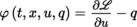 ,
,
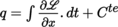 ; φ is of class C
1 and such that
; φ is of class C
1 and such that
 . If the Lagrangian is regular at the point x
*, then, for any t ∈ [t
0, t
1], the implicit function theorem (Theorem 1.30) implies that there exists an open neighborhood of
. If the Lagrangian is regular at the point x
*, then, for any t ∈ [t
0, t
1], the implicit function theorem (Theorem 1.30) implies that there exists an open neighborhood of
 in [t
1, t
2] × Ω1 × Ω2, in which the relation φ (t, x, u, q) = 0 is equivalent to u = ψ (t, x, q), where ψ is of class C
1; thus,
in [t
1, t
2] × Ω1 × Ω2, in which the relation φ (t, x, u, q) = 0 is equivalent to u = ψ (t, x, q), where ψ is of class C
1; thus,
 is of class C
1, and x
* is of class C
2.
is of class C
1, and x
* is of class C
2.
(III) Legendre condition
Suppose that
is of class C
2 and x
* satisfies the Euler–Lagrange equation. Expanding to second order, we have
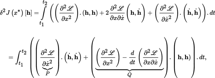
where P and Q are evaluated at the point (t, x * (t)) and h is evaluated at the point t.
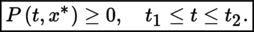
Theorem 1.46
(Legendre) A necessary condition for x
* to minimize J over
is given by the weak Legendre condition:
Proof
Suppose that there exists t
0 ∈ ]t
1, t
2[ such that P(t
0, x
∗(t
0)) ≱ 0. This means that there is v ∈ E
× such that P(t
0, x
* (t
0)). (v, v) = − 2β with β > 0. Since t ↦ P (t, x
* (t)). (v, v) is continuous, there exists a real number α > 0 such that t
1 ≤ t
0 – α < t
0 + α ≤ t
2 and P (t, x
* (t)). (v, v) ≤ − β for all t ∈ [t
0 – α, t
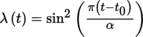
0 + α]. We will construct a function
 for which the above integral is < 0. Let h (t) = λ (t).v with
 for t ∈ [t
0 − α, t
0 + α] and λ (t) = 0 for t ∈ [t
1, t
2] − [t
0 − α, t
0 + α]. It is easy to see that λ is of class C
1 in [t
1, t
2] and (exercise)
for t ∈ [t
0 − α, t
0 + α] and λ (t) = 0 for t ∈ [t
1, t
2] − [t
0 − α, t
0 + α]. It is easy to see that λ is of class C
1 in [t
1, t
2] and (exercise)
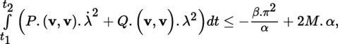
where M = sup
t ∈[t1, t2] Q (t, x
* (t)).(v, v). For α sufficiently small, the right-hand side is < 0. After replacing h by ε.h if necessary, where ε > 0 is sufficiently small, x
* (t) + ε.h (t) ∈ Ω1 and
 for all t ∈ [t
1, t
2]. The necessity of the weak Legendre condition then follows from Theorem 1.42.
for all t ∈ [t
1, t
2]. The necessity of the weak Legendre condition then follows from Theorem 1.42.
1.3.3 “Convenient” differentials
(I)
 topology Let E be a real locally convex space and suppose that A is a non-empty subset of E. A smooth curve in A is defined as a mapping c : I → A of class C
∞, where I is a non-empty open interval of
, for example ]−1, 1[. Any such curve is said to be analytic if it is of class C
ω
.
topology Let E be a real locally convex space and suppose that A is a non-empty subset of E. A smooth curve in A is defined as a mapping c : I → A of class C
∞, where I is a non-empty open interval of
, for example ]−1, 1[. Any such curve is said to be analytic if it is of class C
ω
.
If E is a complex locally convex space, suppose again that A is a non-empty subset of E. Then, A can be viewed as a subset A 0 of the real locally convex space E 0 obtained from E by restriction of the field of scalars ([P2], section 3.2.2 (II)), and any smooth curve in A 0 is said to be a smooth curve in A.
Definition 1.48
[KRI 97] Let E be a locally convex space. The topology
of E is the finest topology that makes all smooth curves in E (
section 1.3.3
) continuous. When equipped with this topology, the space E is denoted by
 .
.
The topology of
is finer than the topology of E, so every open subset of E is open in
. If the space E is bornological ([P2], section 3.4.4
(I), Definition 3.61), it has the finest locally convex topology of all locally convex topologies coarser than the topology of
([KRI 97], Corollary 4.6). “Convenient” differential calculus is performed with mappings defined in open sets of
.
Recall that every Fréchet space and every Silva space is bornological and complete ([P2], sections 3.4.4 (I) and 3.8.2(II)). We have the following result ([KRI 97], Theorem 4.11):
Theorem 1.49
Let E be a metrizable locally convex space or a Silva space. Then, the topology of E coincides with the topology of
.
Remark 1.50
If a locally convex space E is bornological but non-normable, then
 is not a topological vector space (
[KRI 97]
, Corollary 4.21).
is not a topological vector space (
[KRI 97]
, Corollary 4.21).
(II)
 spaces
The following definition will be useful:
Definition 1.52
A locally convex space E is called a
space if it is quasi-complete and bornological, and the topologies of E and
coincide.
Theorem 1.49 shows that Fréchet (and in particular Banach spaces) and Silva spaces are
spaces. Any quasi-complete locally convex space, and hence any
space, is convenient (exercise). Nonetheless,
spaces are sufficiently general for our purposes, so we will restrict attention to them to simplify the statements of results.
(II) Mappings of class

Definition 1.53
Let E and F be real locally convex
spaces and let A be an open subset of E. A mapping f from A into F is said to be of class
if f ∘ c is a smooth curve in F for any smooth curve c in A. This mapping f is said to be of class
 if it is of class
and f ∘ c is an analytic curve in F for every analytic curve c in A.
11
if it is of class
and f ∘ c is an analytic curve in F for every analytic curve c in A.
11
If E is a Banach space and f is of class C
r
(r ∈ {∞, ω}), then f is of class
 . J. Boman showed the following result in 1967 ([KRI 97], Corollary 3.14):
Theorem 1.54
(Boman) Let A be a non-empty open subset of
 . The mapping
 is of class C
∞
if and only if it is of class
.
is of class C
∞
if and only if it is of class
.
Theorem 1.55
Let E and F be
spaces and suppose that A is an open subset of E.
-
1)
Suppose that f : A → F is of class
. Then, f has a Gateaux differential
 at every point of A and the mapping
 is of class
.
is of class
.
-
2)
Let G be a locally convex space and suppose that g : B → G is a mapping of class
, where B is an open subset of F containing f (A). Then, the following chain differentiation rule holds (compare with
[1.5]
and
[1.19]
):

Proof
(1) Let h ∈ E; there exists ε > 0 such that a + t
h ∈ A for all t ∈ ]− ε, + ε[ and the curve t ↦ a + th
is smooth. Therefore, f has a Lagrange first variation δ
f (a). It can be shown that δ
f (a) is bounded linear ([KRI 97], Chapter I, 3.18), so δ
f (a) = D
G
f (a). Furthermore, D
G
f (a) is continuous linear, since E and F are bornological ([P2], section 3.4.4
(I), Theorem 3.62). If c is a smooth curve in A, then δ
f (a) ∘ c is a smooth curve in
 , which gives the stated result by induction (ibid.). (2): ibid.
In the real analytic case, the following result ([KRI 97], Chapter II, section 10.4) generalizes Boman’s theorem:
Theorem 1.56
Let E and F be real
spaces, U a non-empty open subset of E and f : U → F a mapping. The following conditions are equivalent: (i) f is of class
; (ii) f is of class
and λ ∘ f ∘ μ is analytic from Ω into
for any linear form λ ∈ F
∨ and any affine mapping μ : Ω → U (Ω = μ
− 1 (U)).
(III) Holomorphic mappings
Assume that
 .
.
A holomorphic curve in a non-empty open subset A of a complex
space E is a holomorphic mapping from a disk in the complex plane, for example the open disk
 of center 0 and radius 1, into A. A
 -holomorphic mapping (or a mapping of class
) from A into F, where F is a complex
space, is a mapping that transforms the holomorphic curves in A into holomorphic curves in F. With this notation, the mapping f : A → F is holomorphic if and only if λ ∘ f ∘ c is a holomorphic function for every continuous linear form λ ∈ F
∨ and every holomorphic curve
-holomorphic mapping (or a mapping of class
) from A into F, where F is a complex
space, is a mapping that transforms the holomorphic curves in A into holomorphic curves in F. With this notation, the mapping f : A → F is holomorphic if and only if λ ∘ f ∘ c is a holomorphic function for every continuous linear form λ ∈ F
∨ and every holomorphic curve
 . The following result ([KRI 97], Chapter II, section 7.9) generalizes the classical Hartogs theorem ([P2], section 4.3.2
(II), Corollary 4.80):
. The following result ([KRI 97], Chapter II, section 7.9) generalizes the classical Hartogs theorem ([P2], section 4.3.2
(II), Corollary 4.80):
Theorem 1.57
(generalized Hartogs theorem) Let E
1, E
2, F be complex
spaces and suppose that A = A
1 × A
2 is a non-empty open subset of E
1 × E
2. The
mapping f : A → F is -holomorphic if and only if it is
-holomorphic separately in each variable, i.e. f (., z
2) and f (z
1,.) are -holomorphic for every z ∈ A
i
(i = 1, 2).
1.4 Smooth partitions of unity
In this section,
.
1.4.1 C∞ -paracompactness of Banach spaces
Let E be a normed vector space. The topological notions of normal space and paracompact space ([P2], sections 2.3.10 and 2.3.11) inspire the following definitions:
Recall that (ψ i ) i ∈ I is a subordinate partition of unity of (U i ) i ∈ I if and only if supp (ψ i ) ⊂ U i , the family (supp (ψ i )) i ∈ I is locally finite and ∑ i ∈ I ψ i = 1 ([P2], section 2.3.12).
Proof
The necessary condition is clear. We will show the sufficient condition: let (U
i
)
i ∈ I
be an open covering of E. If E is paracompact, there exists a locally finite open covering (V
j
)
i ∈ J
finer than (U
i
)
i ∈ I
such that each V
j
is contained in some U
i(j). There also exist other open refinements (W
j
)
j ∈ J
and (Z
j
)
j ∈ J
of (V
j
)
j ∈ J
such that
 . If E is C
r
-normal, then, for all j, there exists a function ψ
j
: X → [0, 1] of class C
r
that is equal to 1 in
. If E is C
r
-normal, then, for all j, there exists a function ψ
j
: X → [0, 1] of class C
r
that is equal to 1 in
 and 0 in
 . Let ψ = ∑
j
ψ
j
and θ
j
= ψ
j
/ψ. Thus, (θ
j
)
j ∈ J
is a subordinate partition of unity of class C
r
of (V
j
)
i ∈ J
and hence of (U
i(j))
j ∈ J
, which shows that E is C
r
-paracompact.
. Let ψ = ∑
j
ψ
j
and θ
j
= ψ
j
/ψ. Thus, (θ
j
)
j ∈ J
is a subordinate partition of unity of class C
r
of (V
j
)
i ∈ J
and hence of (U
i(j))
j ∈ J
, which shows that E is C
r
-paracompact.
As a metrizable space, every Banach space is paracompact by Stone’s theorem ([P2], section 2.3.10, Theorem 2.57). The next result ([ABR 83], Propositions 5.5.18 and 5.5.19), whose proof was established by Bonic and Frampton in 1966, follows from the fact that any separable Banach space is a Lindelöf space ([P2], section 2.6.3) (exercise).
It was shown in [TOR 73] that every reflexive (not necessarily separable) Banach space is C 1-paracompact and that the separability condition is not required in Corollary 1.62:
This implies the result stated in ([P2], section 4.4.1, Theorem 4.88)
Corollary 1.64
(Whitney’s theorem) The space
is C
∞
-paracompact.
1.4.2
c
∞
-paracompactness
We can define
-regularity,
-normality and
-paracompactness of a locally convex space in the obvious ways; the statement of Theorem 1.59 still holds if C
∞ is replaced by
; moreover, if
is a
-regular Lindelöf space, then it is
-paracompact ([KRI 97], Proposition 16.2). We already know that any nuclear space E has a topology defined by a family of pre-Hilbert norms ([P2], section 3.11.3(III)). Each of these semi-norms is of class
in E − {0}. Nuclear Fréchet spaces (also known as
 spaces), nuclear Silva spaces (also known as
 spaces), and countable products of
spaces and
spaces are paracompact Lindelöf spaces (ibid.). The following result is analogous to Corollary 1.62 ([KRI 97], Theorem 16.10):
spaces), and countable products of
spaces and
spaces are paracompact Lindelöf spaces (ibid.). The following result is analogous to Corollary 1.62 ([KRI 97], Theorem 16.10):
Theorem 1.65
Every
space, every strict inductive limit of
spaces and every
space is
-paracompact.
1.5 Ordinary differential equations
1.5.1 Existence and uniqueness theorems
(I) Notion of the solution of a differential equation
Let I be an interval of
with non-empty interior
 , Ω a non-empty open subset of
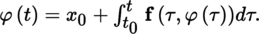
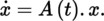
 and f a mapping from I × Ω into E. We say that a mapping φ : I → E is a solution (or integral) of the differential equation
if the conditions (ODE 1,2,3) below are satisfied:
- (ODE 1) φ (t) ∈ Ω for all t ∈ I;
-
(ODE
2) φ is locally absolutely continuous in I (i.e. each of its components with respect to the canonical basis of
is locally absolutely continuous: see [P2], section 4.1.7(III));
-
(ODE
3)
 λ-almost everywhere in I, where λ is the Lebesgue measure on
([P2], section 4.1.1(II)).
λ-almost everywhere in I, where λ is the Lebesgue measure on
([P2], section 4.1.1(II)).
A Cauchy problem involves determining a function φ that is a solution of [1.22] and that satisfies the Cauchy condition:
If φ satisfies the conditions (ODE 1,2,3) and [1.23], then, for all t ∈ I,
Conversely, suppose that [1.24] holds, (ODE 1) is satisfied and t ↦ f (t, φ (t)) is locally λ-integrable. Then, [1.23] holds; furthermore, Lusin’s measurability criterion ([P2], section 4.1.6(II)) implies that the function t ↦ f (t, φ (t)) is λ-measurable for every locally absolutely continuous function φ : I → E if the conditions (Cat 1,2) below are satisfied:
- (Cat 1) the function x ↦ f (t, x) from Ω into E is continuous for every t ∈ I;
- (Cat 2) the function t ↦ f (t, x) from I into E is λ-measurable for every x ∈ Ω.
Suppose further that:
(Cat
3) For all x
0 ∈ Ω and every r > 0 such that B
r
(x
0) ⊂ Ω, where B
r
(x
0) is the open ball of center x
0 and radius r in E, there exists a locally λ-integrable function m from I into
 such that | f (t, x)| ≤ m (t) for all (t, x) ∈ I × B
r
(x
0).
such that | f (t, x)| ≤ m (t) for all (t, x) ∈ I × B
r
(x
0).
Then, for every locally absolutely continuous function φ : I → E satisfying φ (I) ⊂ B r (x 0), the mapping t ↦ | f (t, φ (t))| is locally λ-integrable in I, so t ↦ f (t, φ (t)) is locally λ-integrable in I ([P2], section 4.1.2(I)).
(II) Existence theorem
Proof
We will show that there exist an interval J
β
= [t
0, t
0 + β] ⊂ I (β > 0) and an absolutely continuous mapping φ : J
β
→ E such that φ (J
β
) ⊂ B
r
(x
0) and φ satisfies [1.24]. The same argument works on an interval J′α = [t
0 − α, t
0] (α > 0). Let
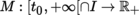 be the mapping:

Since M is continuous and non-decreasing, there exists an interval J β as specified above satisfying the property that, for all t ∈ J β ,
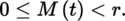
We can now inductively define a sequence of absolutely continuous mappings φ i : J β → E using the conditions:
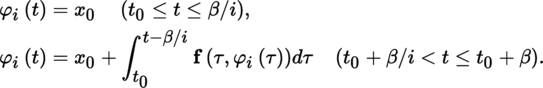
By (Cat 3), the second equation implies that, for all t ∈ J β ,

so φ i (t) ∈ B r (x 0) for all t ∈ J β . If t 1, t 2 ∈ J β , then

and M is uniformly continuous in the compact set J
β
by Heine’s theorem ([P2], section 2.4.5, Theorem 2.86), so | M (t
2 − β/i) − M (t
1 − β/i)| → 0 uniformly in i if t
2 − t
1 → 0, and the set
 is equicontinuous ([P2], section 2.7.3). Since
 is contained in B
r
(x
0) for all t ∈ J
β
, the third Ascoli–Arzelà theorem (ibid.) implies that H is relatively compact in
is contained in B
r
(x
0) for all t ∈ J
β
, the third Ascoli–Arzelà theorem (ibid.) implies that H is relatively compact in
 equipped with the uniform structure of uniform convergence. Hence, there exists a subsequence (φ
i
k
) that converges uniformly to some mapping
. Moreover, | f(t, φ
i
k
(t))| ≤ m(t)(t
0 ≤ t ≤ t
0 + β) and f(t, φ
i
k
(t)) → f(t, φ(t)) for i
k
→ ∞ by (Cat
1); furthermore, as we saw earlier, (Cat
2) implies that t ↦ f (t, φ (t)) is measurable. The Lebesgue dominated convergence theorem ([P2], section 4.1.2(II), Theorem 4.9) therefore implies that, for all t ∈ J
β
,
equipped with the uniform structure of uniform convergence. Hence, there exists a subsequence (φ
i
k
) that converges uniformly to some mapping
. Moreover, | f(t, φ
i
k
(t))| ≤ m(t)(t
0 ≤ t ≤ t
0 + β) and f(t, φ
i
k
(t)) → f(t, φ(t)) for i
k
→ ∞ by (Cat
1); furthermore, as we saw earlier, (Cat
2) implies that t ↦ f (t, φ (t)) is measurable. The Lebesgue dominated convergence theorem ([P2], section 4.1.2(II), Theorem 4.9) therefore implies that, for all t ∈ J
β
,

But, for all t ∈ J β ,

and the second integral tends to 0 as i k → ∞, so the equality [1.24] is satisfied for all t ∈ J β . Finally, φ i k → φ in the Banach space AC (J β ; E) of absolutely continuous mappings from J β into E ([P2], section 4.1.7(III)), so φ is absolutely continuous.
Corollary 1.68
(Peano’s theorem) Suppose that f is continuous in I × Ω. Let J be a compact interval that is a neighborhood of t
0 in I and let
 . For every compact interval [t
0, t
0 + β] contained in J satisfying β < r/m, there exists a solution of
[1.24]
that takes values in B
r
(x
0).
. For every compact interval [t
0, t
0 + β] contained in J satisfying β < r/m, there exists a solution of
[1.24]
that takes values in B
r
(x
0).
Remark 1.69
Corollary 1.68 (and hence
Theorem 1.67
) fails if E is replaced by an arbitrary Banach space ([BOU 76],
Chapter 4
, section 1, Exercise 18). We can define an absolutely continuous mapping φ : J
β
→ E as we did in ([P2], section 4.1.7(I)), but it is not true in general that
 for all t ∈ J
β
(however, this property does hold if E is assumed to be reflexive). Furthermore, since the ball B
r
(x
0) is not relatively compact when E is infinite-dimensional, the proof of
Theorem 1.67
no longer works.
for all t ∈ J
β
(however, this property does hold if E is assumed to be reflexive). Furthermore, since the ball B
r
(x
0) is not relatively compact when E is infinite-dimensional, the proof of
Theorem 1.67
no longer works.
(III) Uniqueness theorem The fourth Carathéodory condition can be stated as follows (reusing some of the notation of Cat 3):
(Cat
4) For all x
0 ∈ E and every real number r > 0 such that B
r
(x
0) ⊂ Ω, there exists a locally λ-integrable function k from I into
such that

Theorem 1.70
(Carathéodory) Suppose that the Carathéodory conditions
Cat
1,2,3,4 are satisfied. Then, for all
 , there exists an interval J ⊂ I with interior point t
0 and a unique mapping φ : J → Ω that is a solution of
[1.22]
and which satisfies the Cauchy condition
[1.23]
.
, there exists an interval J ⊂ I with interior point t
0 and a unique mapping φ : J → Ω that is a solution of
[1.22]
and which satisfies the Cauchy condition
[1.23]
.
Proof
Let
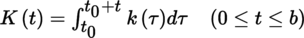
and choose the real number β > 0 in the proof of Theorem 1.67 to satisfy the additional condition K (β) < 1. Furthermore, let

and, for every function
 , set
, set

Clearly,
 . The set
is a closed subset of the space
. The set
is a closed subset of the space
 equipped with the uniform structure of uniform convergence; the norm of
is ‖ψ‖∞ ≔ sup
t ∈ [0, β]| ψ(t)|. The space
is complete ([P2], section 2.7.2, Corollary 2.115), so
is complete ([P2], section 2.4.4(II), Lemma 2.77). Furthermore,
equipped with the uniform structure of uniform convergence; the norm of
is ‖ψ‖∞ ≔ sup
t ∈ [0, β]| ψ(t)|. The space
is complete ([P2], section 2.7.2, Corollary 2.115), so
is complete ([P2], section 2.4.4(II), Lemma 2.77). Furthermore,
 is a fixed point of T if and only if the function
 defined by

satisfies [1.24]; finally, ψ (t – t
0) ∈ B
r
(0) if and only if φ (t) ∈ B
r
(x
0). If
 for all t ∈ [0, β], then
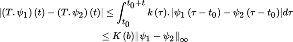
and hence ‖T. ψ 1 − T. ψ 2‖∞ ≤ K(b)‖ψ 1 − ψ 2‖∞. Therefore, T has a unique fixed point by Theorem 1.27.
Definition 1.71
-
1)
We say that f : I × Ω → E is locally Lipschitz in the second variable in I × Ω if, for every (t, x) ∈ I × Ω, there exists a neighborhood V of t, a neighborhood S of x and a constant k
V,S
> 0 such that f (., x) is regulated on V (
[DIE 93]
, Volume 1, section 7.6) and f satisfies the Lipschitz condition:
- 2) We say that f is Lipschitz with constant k > 0 in the second variable if the above statement is satisfied when V = I, S = Ω and k V,S = k.

Any locally Lipschitz function in the second variable clearly satisfies the conditions Cat 1,2,3,4, and we may therefore apply Theorem 1.70 to this function. We also have the following result:
Corollary 1.72
(Cauchy–Lipschitz theorem) If f is Lipschitz with constant k in the second variable in I × Ω, let J be a compact interval contained in I with non-empty interior, t
0 a point of
, x
0 a point of E, r > 0 a real number such that B
r
(x
0) ⊂ Ω,
and ρ = min {r/m, 1/k}. For every compact interval K contained in J ∩ ]t
0 − ρ, t
0 + ρ[, there exists a unique mapping φ that is a solution of
[1.22]
and which satisfies the
Cauchy condition
[1.23]
.
Theorem 1.74
Let E be the space
(respectively any Banach space),
 an interval with some interior point t
0, Ω a non-empty open subset of E and f : I × Ω → E a mapping satisfying the conditions
Cat
1,2,3,4 (respectively a locally Lipschitz function in the second variable). For all x
0 ∈ Ω, there exists a maximal interval J (t
0, x
0) ⊂ I with interior point t
0 in which
[1.22]
has a solution φ satisfying the Cauchy condition
[1.23]
and such that φ (J (t
0, x
0)) ⊂ Ω. This solution φ (.; t
0, x
0) is unique.
an interval with some interior point t
0, Ω a non-empty open subset of E and f : I × Ω → E a mapping satisfying the conditions
Cat
1,2,3,4 (respectively a locally Lipschitz function in the second variable). For all x
0 ∈ Ω, there exists a maximal interval J (t
0, x
0) ⊂ I with interior point t
0 in which
[1.22]
has a solution φ satisfying the Cauchy condition
[1.23]
and such that φ (J (t
0, x
0)) ⊂ Ω. This solution φ (.; t
0, x
0) is unique.
Proof
Let
 be the set of intervals L ⊂ I with non-empty interior containing t
0 as an interior point and such that there exists a solution φ of [1.22] in L satisfying the Cauchy condition [1.23] and φ (L) ⊂ Ω. The set
is not empty by Theorem 1.70 (respectively Corollary 1.72 and Remark 1.73). Let
be the set of intervals L ⊂ I with non-empty interior containing t
0 as an interior point and such that there exists a solution φ of [1.22] in L satisfying the Cauchy condition [1.23] and φ (L) ⊂ Ω. The set
is not empty by Theorem 1.70 (respectively Corollary 1.72 and Remark 1.73). Let
 with L ⊂ L′. If φ, φ′ are solutions of [1.22] in L, L′, respectively, satisfying the Cauchy condition [1.23], then it follows from Theorem 1.70 (respectively Corollary 1.72 and Remark 1.73) (arguing by contradiction: exercise) that φ′ is a continuation of φ. Let
 ; there must therefore exist a unique solution φ of [1.22] in J (t
0, x
0) satisfying the Cauchy condition [1.23] and φ (J (t
0, x
0)) ⊂ Ω.
; there must therefore exist a unique solution φ of [1.22] in J (t
0, x
0) satisfying the Cauchy condition [1.23] and φ (J (t
0, x
0)) ⊂ Ω.
(IV) Differential equations in implicit form
Let I be an open interval of
, t
0 a point of I, F a Banach space and Ω a non-empty open subset of F
n + 1, where n is a natural integer. Let g : I × Ω → F be a mapping of class C
1 and consider the differential equation:
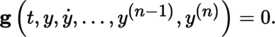
Let η 0 = (η 0 0, η 0 1,…, η 0 n − 1) ∈ F n and ξ 0 ∈ F such that (η 0, ξ 0) ∈ Ω, g (t 0, η 0, ξ 0) = 0, and suppose that the following condition (Inv) is satisfied:
(Inv)
 is invertible in
 .
.
By the implicit function theorem (Theorem 1.30), there exists an open neighborhood J × U of (t 0, η 0) in I × F n , an open neighborhood V of ξ 0 in F, where U × V ⊂ Ω, and a mapping h : J × U → V of class C 1, such that, for all (t, η, ξ) ∈ J × U × V,

Therefore, any mapping ψ : J → F such that
 and ψ
(n) (t) ∈ V for all t ∈ J is a solution of [1.26] in J if and only if ψ is a solution of the following differential equation on J, said to be in explicit form:
and ψ
(n) (t) ∈ V for all t ∈ J is a solution of [1.26] in J if and only if ψ is a solution of the following differential equation on J, said to be in explicit form:
Let x i = y (i − 1) (i = 1,…, n) and x =(x 0, …, x n ). For (t, x) ∈ J × U × V, the differential equation [1.27] is equivalent to [1.22], where f = (f 1,…, f n ) and

The mapping f : J × U → F n is of class C 1 and hence locally Lipschitz in x by the mean value theorem (Theorem 1.13(i)). We can therefore apply Theorem 1.72 according to Remark 1.73. Let x 0 = (η 0 1, …, η 0 n − 1); any solution φ = (φ 0, …, φ n ) of [1.22] of class C 1 in J satisfies the Cauchy condition [1.23] if and only if φ = φ 1 is a solution of [1.26], of class C n in J and ψ (t 0) = η 0 1, …, ψ (n − 1) (t 0) = η 0 n − 1.
1.5.2 Linear differential equations
(I) Let I be an interval of
with non-empty interior
and let
. Consider the linear differential equation
where
 and b : I → E are locally λ-integrable. The Carathéodory conditions Cat
1,2,3,4 are all satisfied. (In particular, setting f (t, x) = A (t).x + b (t), we have
and b : I → E are locally λ-integrable. The Carathéodory conditions Cat
1,2,3,4 are all satisfied. (In particular, setting f (t, x) = A (t).x + b (t), we have

which shows that Cat
4 is satisfied.) Hence, for all
 and every x
0 ∈ E, there exists a unique solution φ (.; t
0, x
0) of [1.28] in I satisfying [1.23].
and every x
0 ∈ E, there exists a unique solution φ (.; t
0, x
0) of [1.28] in I satisfying [1.23].
The linear equation [1.28] is said to be homogeneous if b = 0, in which case
(II) The set of solutions of [1.29] (where A is locally λ-integrable) is an
-vector space. Let φ
0 (.; t
0, x
0) be a solution of [1.29] in I satisfying [1.23]. The mapping x
0 ↦ φ
0 (t; t
0, x
0) is a bijective linear mapping Φ (t, t
0) from E onto E, and Φ(., t
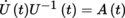
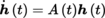
0) is identical to the solution of the differential equation
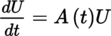
for U (t 0) = 1 E . For all t 1, t 2, t 3 ∈ I, we have Φ(t 3, t 1) = Φ (t 3, t 2) ∘ Φ(t 2, t 1) and Φ(t 1, t 2) = Φ(t 2, t 1)− 1.
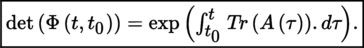
Proof
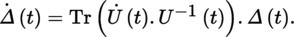
Set Φ(t, t
0) = U (t), Δ(t) = det (U (t)) and write U (t + h) = U (t) + h.V + o (h), where
 . Then, Δ(t + h) = Δ (t).det (I + h.V.U
− 1 (t) + o (h)). But
. Then, Δ(t + h) = Δ (t).det (I + h.V.U
− 1 (t) + o (h)). But

Furthermore, by [P1], section 2.3.11 (VII),

so det (I + h.V.U − 1 (t) + o(h)) = 1 + h.Tr (V.U − 1 (t)) + o (h). Hence, Δ(t + h) = Δ (t).(1 + h.Tr (V.U − 1 (t 0)) + o (h)), so
We now simply apply the relation
 , which follows from [1.30].
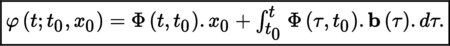
(III) The above shows that the general solution of [1.29] is of the form t ↦ Φ(t, t 0)ξ. The “variation of constants” method (exercise) allows us to obtain the following solution (defined in I) of [1.28] and the Cauchy condition [1.23]:
(IV) The integration of linear differential equations with constant coefficients is a classical problem and is performed using the Jordan normal form ([P1], section 3.4.3 (IV)): see, for example, [BOU 10], section 12.5.2.
1.5.3 Parameter dependence of solutions
Let I be an interval of
with non-empty interior, E a Banach space (see Remark 1.73), Ω a non-empty open subset of E, Λ a topological space and f a mapping from I × Ω × Λ into E. Write f
λ
(t, x) for the value of f at the point (t, x, λ) ∈ I × Ω × Λ. It is possible to show the following result ([BOU 76], Chapter 4, section 1.6, Theorem 3):
Theorem 1.80
(parameter dependence of solutions) Suppose that, for all λ ∈ Λ, (t, x) ↦ f
λ (t, x) is Lipschitz in the second variable x in I × Ω and that f
λ
(t, x) → f
λ
0
(t, x) uniformly in I × Ω as λ → λ
0. Let φ
λ
0
be a solution of
 satisfying the Cauchy condition
 , defined on an interval J = [t
0, t
0 + β[ ⊂ I and taking values in Ω. For every compact interval [t
0, t
1] ⊂ J, there exists a neighborhood V of λ
0 in Λ such that, for all λ ∈ V, the differential equation
, defined on an interval J = [t
0, t
0 + β[ ⊂ I and taking values in Ω. For every compact interval [t
0, t
1] ⊂ J, there exists a neighborhood V of λ
0 in Λ such that, for all λ ∈ V, the differential equation
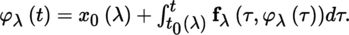
admits a unique solution φ λ defined in [t 0, t 1] satisfying the Cauchy condition φ λ (t 0) = x 0 and taking values in Ω; furthermore, as λ → λ 0, φ λ → φ λ 0 uniformly in [t 0, t 1].
Suppose now that Λ is an open subset of a normed vector space F and that the mapping (t, x, λ) ↦ f
λ (t, x) is continuous with continuous partial differentials
13
 and
and
 . Then, f
λ
is locally Lipschitz in the second variable x (see section 1.5.1
(V)). Suppose further that the mappings x
0 : Λ → Ω: λ → x
0 (λ) and t
0 : Λ → I : λ ↦ t
0 (λ) are of class C
1 in Λ. For all λ
ο ∈ Λ, Theorem 1.80 implies that there exist an open neighborhood V of λ
0 in Λ and an open interval J ⊂ I such that t
0 (λ
0) ∈ J, where the sets V and J satisfy the following condition: for all λ ∈ V, t
0 (λ) ∈ J and there exists a solution φ
λ
= φ (.,t
0 (λ), x
0 (λ)) of [1.31] in J taking the value x
0 (λ) ∈ Ω at the point t
0 (λ). Then, we have the following result:
. Then, f
λ
is locally Lipschitz in the second variable x (see section 1.5.1
(V)). Suppose further that the mappings x
0 : Λ → Ω: λ → x
0 (λ) and t
0 : Λ → I : λ ↦ t
0 (λ) are of class C
1 in Λ. For all λ
ο ∈ Λ, Theorem 1.80 implies that there exist an open neighborhood V of λ
0 in Λ and an open interval J ⊂ I such that t
0 (λ
0) ∈ J, where the sets V and J satisfy the following condition: for all λ ∈ V, t
0 (λ) ∈ J and there exists a solution φ
λ
= φ (.,t
0 (λ), x
0 (λ)) of [1.31] in J taking the value x
0 (λ) ∈ Ω at the point t
0 (λ). Then, we have the following result:
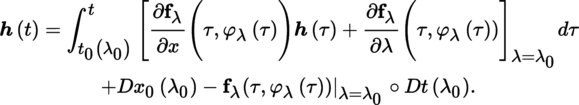
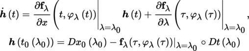
Theorem 1.81
For every t ∈ J, the mapping λ ↦ φ
λ
(t) from V into Ω has a differential
 at the point λ
0 of V ; h is of class C
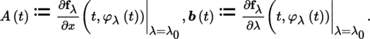
1 in J and is the unique solution of the linear equation:
at the point λ
0 of V ; h is of class C
1 in J and is the unique solution of the linear equation:
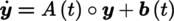
where
This differential h satisfies the Cauchy condition:

Proof
For all t ∈ J,
Hence, by [DIE 93], Volume 1, section 8.11, (8.11.2) and Problem 1,
Therefore, h is of class C 1 in J and
Note that, in the linear equation [1.32],
 ; moreover,
y
, A(t) ∘
y
, and
b
(t) belong to
; moreover,
y
, A(t) ∘
y
, and
b
(t) belong to
 . In the Cauchy condition, f
λ
(t
0
λ),
. In the Cauchy condition, f
λ
(t
0
λ),
 ,
,
 ,
,
 , and f
λ (t
0 (λ),
, and f
λ (t
0 (λ),
 .
.
Corollary 1.82
(differentiability of the solution with respect to x 0) Suppose that F = E, Λ = Ω, and λ = x 0, and adopt the same hypotheses as Theorem 1.81 (mutatis mutandis). Write f and φ for f λ and φ λ respectively. Then:
where Φ is the resolvent ( Definition 1.78 ) of the linear differential equation

Proof
By Theorem 1.81,
 and
h
(t
0) = 1
E
.
and
h
(t
0) = 1
E
.
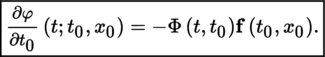
Corollary 1.83
(differentiability with respect to the initial time) Suppose that
 , Λ = I, and λ = t
0
. With the notation of
Corollary 1.82
and the same hypotheses (exercise):
, Λ = I, and λ = t
0
. With the notation of
Corollary 1.82
and the same hypotheses (exercise):
Remark 1.84
Let E be finite-dimensional. The statement of Corollary 1.82 still holds under the weaker condition ( [ALE 87] , Chapter 2 ,section 2.5.6) that f satisfies the Carathéodory conditions ( Cat 1,2,3 ) and Lusin’s condition (L) holds:
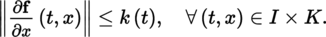
(L): For all t ∈ I, the mapping x ↦ f (t, x) is continuously differentiable on Ω and, for every compact set K ⊂ Ω, there exists a locally λ-integrable function
 such that
It is clear that condition (L) implies (Cat 4 ) by the mean value theorem. This condition does not require f to be continuous in t, which is very important in optimal control theory (Pontryagin maximum principle): see op. cit. and [PON 62] . We can further weaken (L) by considering generalized gradients and differential inclusions ( [CLA 90] ,Theorem 7.4.1), but this exceeds the scope of the present book.