Chapter 6. Classification and Regression

A key ingredient for successful machine learning implementations (based on discussions with many data scientists, machine learning engineers, and product managers) is being able to map the business problem and the desired outcome to the appropriate machine learning problem (or having a frank conversation that machine learning will not solve the problem!). Classification and regression are two common machine learning techniques that are used.

In this chapter, we cover the basics of classification and regression and show you how to map a business use case to a classification or regression problem. You’ll learn how to use Microsoft Azure Machine Learning—specifically, automated ML—to automatically select the best classification or regression models for your specific use case.

Tip

Need to Get Started with Azure Machine Learning?

If you’re getting started with Azure Machine Learning, refer to Chapter 3 to understand the basic concepts before diving into this chapter.

What Is Classification and Regression?

In supervised learning, you have a set of independent features, X, and a target feature, Y. The machine learning task is to map from X → Y. Both classification and regression are supervised learning, with a requirement on the availability of labeled data.

To train a high-quality model that performs well for testing data and for generalizing new unseen data, examples need to be sufficiently representative of the test data. One underlying assumption for many supervised learning algorithms is that the data distribution of training examples is identical to that of the test examples (including unseen examples).

In many real-world problems, this is often untrue. Either your data has very few objects with the target feature that you want to predict (known as the class imbalance, or the minority class problem), or it isn’t of good quality. In some situations, you might not even have labeled data! Over the years, the machine learning community has invented clever ways to deal with each of these problems (e.g., using the Synthetic Minority Oversampling Technique, or SMOTE, to deal with class imbalance), but it’s beyond the scope of this book to go into detail about them.

When Y is a discrete feature, and you’re trying to predict the class/label, you are dealing with a classification problem. Classification helps predict which category (or class) an object belongs to. When classification is used for data with two distinct classes, we often refer to it as binary classification. If there are more than two distinct classes, it is a multiclass classification problem. For example, predicting whether a person is a good or bad credit risk is a binary classification problem (because there are two distinct classes: good or bad). Predicting a book category (e.g., fairytale, cookbook, biography, travel, and so on) is a multiclass classification problem.

When Y is a continuous feature that you are trying to predict, you are dealing with a regression problem. Regression helps to predict a continuous value. For example, in manufacturing’s predictive maintenance scenarios, regression models are used to predict the lifespan for systems and equipment. In health care, regression is used to predict health-care costs, length of hospital stays for patients, and more. Figure 6-1 shows a typical data science process for training and evaluating machine learning models. The same workflow applies to both classification and regression problems.

Figure 6-1. Training a classification/regression model

Data is first split into training and testing data. The training data is used as inputs to a classification/regression algorithm. A machine learning model is produced once training completes, after which it’s The evaluated using the test data. As part of model evaluation, you’ll compute different types of metrics (e.g., precision, accuracy, AUC, F1-score, and so on), which helps you determine its quality.

Let’s illustrate this with an example on credit-risk scoring. In financial services, credit-risk scoring enables a bank to make credit decisions for customers. The German Credit Risk dataset consists of 1,000 rows (Table 6-1 shows a subset of the dataset). Each row uses a set of features (or attributes, or properties) to describe a person. The last column is the class/label (i.e., Credit Risk), which provides information on whether the person is a credit risk.

Note

The German Credit Risk dataset is available in the UCI Machine Learning Repository. The dataset was contributed to the machine learning community in 1994 by Professor Hans Hofmann and consists of 20 features (7 numerical, 13 categorical), and one credit risk label.

Download the file german.data from the UCI Machine Learning Repository:

import pandas as pd
columns = ['status_checking_acc', 'duration_months', 'credit_history',
     'purpose', 'credit_amount', 'saving_acc_bonds',
     'present_emp_since','installment_rate', 'personal_status',
     'other_debtors', 'residing_since', 'property', 'age_years',
     'inst_plans', 'housing', 'num_existing_credits', 'job',
     'dependents', 'telephone', 'foreign_worker', 'status']

creditg_df = pd.read_csv(
     'https://archive.ics.uci.edu/ml/machine-learning-databases/statlog
                                    /german/german.data',
delim_whitespace = True, header = None )
# Assign the header row to
creditg_df.columns = columns

# Get the initial rows of data
creditg_df.head()

After you download the data, observe that in each row, the first few columns (e.g., existing account status, duration, credit history, foreign worker) describe different personal attributes. In Table 6-1, you can see that the first column shows the account status for the person’s checking account. A11 through A13 denote the amount available in the checking account (amounts are in DM, Deutsche Marks, the German currency until 2002). A14 indicates that the person has no checking account. For illustration purposes, we omitted many features. The last column shows the credit risk: a value of 1 indicates no credit risk, and 2 indicates a credit risk.

Table 6-1. German Credit Risk dataset

Existing account status	Duration (months)	Credit history	…	Foreign worker	Credit risk
A11	6	A34	…	Yes	1
A12	48	A32	…	No	1
A14	12	A34	…	No	2
A11	42	A32	…	Yes	1

Before we dive deeper into the German Credit Risk dataset, let’s review classification and regression algorithms.

Classification and Regression Algorithms

A rich set of classification and regression algorithms has been developed over the years by the machine learning community. Commonly used classification algorithms include the naïve Bayes classifier, support vector machines (SVMs), k-nearest neighbor, decision tree, and random forest. For regression, decision trees, elastic nets, LARS Lasso, stochastic gradient descent (SGD), and SVMs, are commonly used.

If you’re asking which classification/regression algorithm should I be using?, the answer is: it depends. Often, a data scientist tries different algorithms (depending on the problem, the dataset size, requirements for explainable models, speed of the algorithms, and more). The trade-off is often between speed, model evaluation metrics (e.g., accuracy), and explainable results.

For example, if you’re looking at the computational speed at which the initial solution arrives, you might consider decision trees (or any tree-based variant) or simple linear regression approaches. However, if you’re optimizing for accuracy (and other metrics), you might use random forests, SVMs, or gradient boosting trees. Often, the best result is an ensemble of different classification/regression models.

Tip

For a deeper dive into how each classification algorithm works, refer to Professor Tom Mitchell’s Machine Learning course, which provides a fantastic discussion on the different machine learning algorithms.

New to machine learning? Refer to this Microsoft cheat sheet for the different classification algorithms and the use cases in which they can be applied.

Figure 6-2 shows an example of a possible decision tree that is trained using the German Credit Risk dataset. You will notice that the tree starts with a split attribute–account status. If the values for account status are A13, A14, the person doesn’t present a credit risk. The tree further chooses other split attributes (duration and credit history) and uses this to further determine whether a person is a credit risk.

Figure 6-2. Decision tree for the German Credit Risk dataset

Each of these classification algorithms has hyperparameters that need to be tuned. Also, the data distribution, dimensionality of data, sparseness of data, and whether the data is linearly separable matter. As data scientists mature in their practice, they build their toolboxes and knowledge of the algorithms to use (based on familiarity with how the algorithms work, and how to tune the hyperparameters).

If you are interested in experimenting with different classification algorithms and datasets, scikit-learn provides a rich library of various classification algorithms and is a good Python machine learning library to get started with.

Using Automated ML for Classification and Regression

Let’s begin to get our hands dirty with a classification problem. To jumpstart your learning of using automated ML for classification of credit risks using the German Credit Risk dataset, you can use the notebook provided on GitHub and run them using Microsoft Azure Notebooks.

Though automated ML seems almost magical (i.e., given a dataset, perform some auto feature engineering, enumerate through different types of models, and select the best model), having the right input data will help significantly improve the quality of the models.

Tip

The sample notebook for using automated ML with Azure Machine Learning to train a credit risk model is available at https://bit.ly/2m3xlyP.

A rich set of classification and regression algorithms is supported when using automated ML, as shown in Table 6-2.

Table 6-2. Classification and regression algorithms supported by automated ML in Azure Machine Learning

Type of algorithm	Classification	Regression
C-SVC	✓
Decision tree	✓	✓
Elastic net		✓
Extremely randomized trees	✓	✓
Gradient boosting	✓	✓
k-nearest neighbors	✓	✓
LARS Lasso		✓
Light GBM	✓	✓
Linear SVC	✓
Logistic regression	✓
Naïve Bayes	✓
Random forest	✓	✓
SGD	✓	✓

Note

To get the updated list of classification algorithms supported by automated ML, and to understand details about how each algorithm works, refer to this Microsoft documentation.

Setting up the Azure Machine Learning workspace

Previously, you learned how to set up your Azure Machine Learning workspace and prepared the configuration file with the subscription ID, resource group, and workspace name. Use the following code to set up that configuration file:

config.json
{
    "subscription_id": "<Replace with Azure Subscription ID>",
    "resource_group": "oreillybook",
    "workspace_name": "automl-tutorials"
}

When using Azure Notebooks, the config.json file should be stored in the same folder or in the aml_config folder, as shown in Figure 6-3.

Figure 6-3. Getting started with running Azure Notebooks

After you’ve uploaded these files to Azure Notebooks or your own local Jupyter Notebook environment, you are ready to get started. Let’s begin by importing the relevant Python packages that you will use in this exercise:

import numpy as np
import pandas as pd
from sklearn.model_selection import train_test_split
import logging

Next, import the Azure Machine Learning SDK (azureml-sdk):

import azureml.core
from azureml.core.experiment import Experiment
from azureml.core.workspace import Workspace
from azureml.train.automl import AutoMLConfig

After you’ve imported the relevant Python packages, you will create the Azure Machine Learning workspace using the values from config.json.

Workspace.from_config() reads the config.json file, which is either stored in either the same folder as the notebook or aml_config/config.json. As discussed in earlier chapters, the workspace object stores information about the Azure subscription, and information about various resources used. After you create it, it also creates a cloud resource that monitors and tracks the model runs:

ws = Workspace.from_config()

# Populate a workspace info object
workspace_info = {}
workspace_info['SDK version'] = azureml.core.VERSION
workspace_info['Subscription ID'] = ws.subscription_id
workspace_info['Workspace Name'] = ws.name
workspace_info['Resource Group'] = ws.resource_group
workspace_info['Location'] = ws.location
pd.set_option('display.max_colwidth', −1)
workspace_info = pd.DataFrame(data = workspace_info, index = [''])
workspace_info.T

After you run the Python code, you will see the output shown in Figure 6-4, which provides information about the version of the Azure Machine Learning SDK, the Azure subscription ID, and the name and location of the Azure Machine Learning workspace that’s been created.

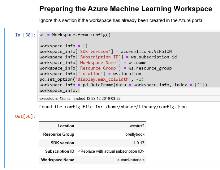
Figure 6-4. Preparing the Azure Machine Learning workspace

If this is the first time you are running the code in Azure Notebooks, you might see the following warning message:

Warning: Falling back to use azure cli login credentials. If you run your
code in unattended mode, i.e., where you can't give a user input, then
we recommend to use ServicePrincipalAuthentication or MsiAuthentication.

Found the config file in: /home/nbuser/library/config.json Performing
interactive authentication. Please follow the instructions on the terminal.

To sign in, use a web browser to open the page https://microsoft.com/devicelogin
and enter the code <9-digit code> to authenticate.

To authenticate with Azure, click https://microsoft.com/devicelogin and enter the authentication code that is provided. After you have logged in using a valid credential, you can rerun the cell, and you will be authenticated.

To run the code as part of an unattended operation, you’ll need to set up an Azure Service Principal and use that to log in programmatically. To learn more about how to authenticate with Azure Machine Learning, visit this GitHub repository.

Next, after you’ve created the Azure Machine Learning workspace, you need to create the experiment object that will be used for this exercise. In the code that follows, notice that we pass the reference to the workspace object that we created earlier when creating the experiment. We also specify a project folder to contain the list of files that will be created, as shown in Figure 6-5.

# Choose the experiment name and specify the project folder.

experiment_name = 'automl-classification'
project_folder = './book/automl-classification'

experiment = Experiment(ws, experiment_name)

Figure 6-5. Creating the experiment and specifying the project folder

Data preparation

For this exercise, we’re using data from the UCI Machine Learning Repository, which contains a rich collection of datasets for both classification and regression problems. Another good repository of open machine learning datasets is OpenML.org. The German Credit Risk dataset is available in both dataset repositories.

Because the german.data file from the UCI Machine Learning Repository does not contain a header row, we first define the names of each of the columns. This helps us reference the column names as we work with the dataset. After the following code is executed, you’ll see the first five rows of the dataset shown in Figure 6-6, in which each row has 21 columns, with the last column being the label column, named Status:

# Define the column
columns = ['status_checking_acc', 'duration_months', 'credit_history',
           'purpose', 'credit_amount','saving_acc_bonds',
           'present_emp_since', 'installment_rate','personal_status',
           'other_debtors', 'residing_since', 'property',
           'age_years','inst_plans', 'housing', 'num_existing_credits',
           'job', 'dependents', 'telephone', 'foreign_worker', 'status']

creditg_df = pd.read_csv(
            'https://archive.ics.uci.edu/ml/
    machine-learning-databases/statlog/german/german.data',
    delim_whitespace = True, header = None )
creditg_df.columns = columns
creditg_df.head()

Figure 6-6. Specifying the name of the columns and loading the data

The Status column is the class that we are trying to build a model for predicting. Let’s look at the number of unique values for the Status column. The values in the status column are 1 and 2; 1 denotes good credit, and 2 denotes bad credit. To make it easier to read, we subtract 1 from the values so that we use a value of 0 to represent good credit, and 1 to represent that the person has bad credit:

# Get the unique values in the Status Column
creditg_df.status = creditg_df.status − 1
creditg_df['status'].unique()

In addition, we also separated out the column with the target feature:

# Get the label column, and remove the label column from the dataframe
# When axis is 1, columns specified are dropped

target = creditg_df["status"]
creditg_df =  creditg_df.drop(labels='status',axis=1)

We are now ready to split the data into train and test data. In this exercise, we do a 70/30 split (i.e., 70% of the data for training, and the remainder for testing). In the following code, you can see that we pass in the reference for the target column, as well, when we call train_test_split:

# Split into train and test data
X_train, X_test, y_train, y_test =
    train_test_split(creditg_df, target, test_size=0.3)

# Convert y_train and y_test from Pandas Series to ndArray
y_train = y_train.values
y_test = y_test.values

After you have split the data into train and test data, you should double-check both DataFrames—X_train and X_test.

Both DataFrames should have 20 columns, as shown in Figure 6-7. Because train_test_split returns the training and testing label columns as Pandas Series (denoted by y_train, and y_test), we can convert both of these objects to either ndArray or DataFrame. This will be used as one of the inputs to the AutoMLConfig object that will be created.

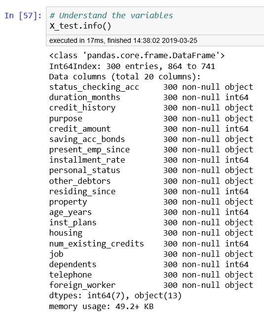
Figure 6-7. Information about DataFrame X_test

Using automated ML to train the model

We are ready to use automated ML to train the classification model for the German Credit Risk problem.

But before we do that, let’s look at the metrics available for tuning when using automated ML, by using the function get_primary_metrics(). Figure 6-8 shows the output. You’ll see that the common classification metrics are supported. These include accuracy, precision, AUC, and the weighted precision scores:

# Explore the metrics that are available for classification
azureml.train.automl.utilities.get_primary_metrics('classification')

Figure 6-8. Metrics used for classification models

Let’s define the common automated ML settings used in multiple experiments:

import time
automl_settings = {
    "name": "AutoML_Book_CH08_Classification_{0}".format(time.time()),
    "iteration_timeout_minutes": 10,
    "iterations": 30,
    "primary_metric": 'AUC_weighted',
    "preprocess": True,
    "max_concurrent_iterations": 10,
    "verbosity": logging.INFO
}

Next, we create the AutoMLConfig object that specifies the automated ML settings and the training data (including the label column y_train). We specify the number of cross-validations to be performed as 5:

automl_config = AutoMLConfig(
                   task = 'classification',
                   debug_log = 'automl_errors.log',
                   X = X_train,
                   y = y_train,
                   n_cross_validations = 5,
                   path = project_folder,
                   **automl_settings
                 )

Tip

When creating the AutoMLConfig object, you will notice that in this example, we specify the task as classification. If you are using automated ML for automatically selecting the best regression models, you should specify the task as regression.

To find out about the various knobs that you can use when creating the AutoMLConfig object, refer to https://bit.ly/2lZWXwo. You can use whitelist_models to specify a list of algorithms to be used when searching for the best model with automated ML. You can also specify the list of models that are ignored in the experiment iteration by using blacklist_models.

After you’ve created the AutoMLConfig object, you are ready to submit the experiment, as follows:

local_run = experiment.submit(automl_config, show_output = True)

When the experiment has been submitted, automated ML will run and evaluate several iterations. Each iteration will use different classification algorithms as well as auto-featurization techniques, and show you the evaluation metrics. The best iteration score will also be shown. Figure 6-9 shows the output from the 30 iterations that are evaluated.

Notice that iteration 14, which uses logistic regression, achieved the best model score of 0.7727 initially. And in iteration 30 (the last one), an ensemble was used, which improved the best model score from 0.7727 to 0.7916. You will also see the explanation for each column shown in the experiment output (e.g., SAMPLING %, DURATION, METRIC, BEST).

When the experiment has completed successfully, you can view the details of the run in the Azure portal:

local_run

Or by using the automated ML Jupyter Notebook widgets:

import azureml.widgets
from azureml.widgets import RunDetails
RunDetails(local_run).show()

Tip

If you have not installed the Python package for the widget, you can also pip install azureml-widgets.

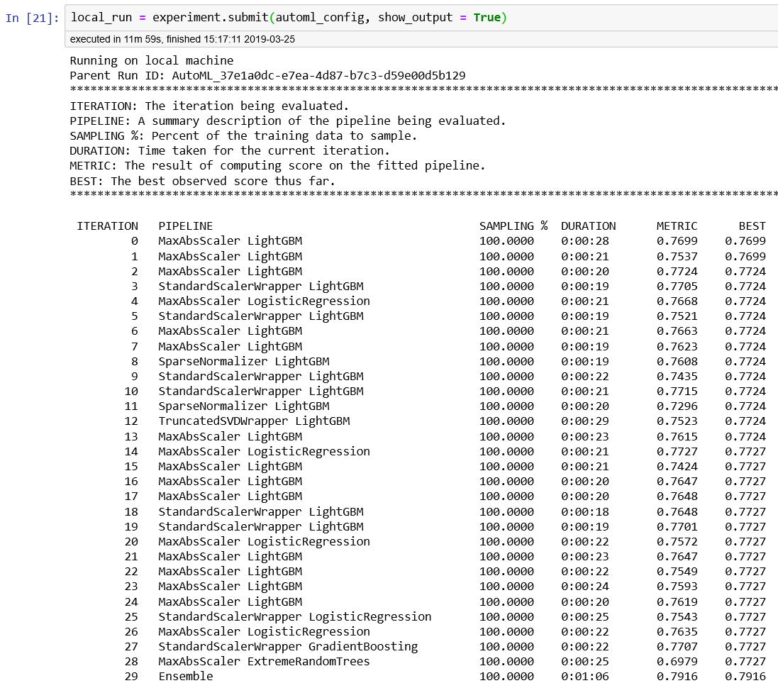
Figure 6-9. Output from submitting the automated ML classification experiment

As shown in Figure 6-10, if you click Link to Azure Portal, you will see the details from the latest run that you have completed. You can also deep dive into the logs that are created from running the experiments.

Figure 6-10. Getting information about local_run

Figure 6-11 shows the details for the run, with run number 347. From the chart, you can see the performance of a model in each iteration of the run.

Figure 6-11. Azure portal—details for a run of an experiment

Once you install the widgets, you’re ready to see the run details directly in Azure Notebooks.

Figure 6-12 shows the output from RunDetails(local_run).show(). You can also click each iteration to view more details. For example, if you click the last iteration (shown as the first row) for Ensemble, you will see detailed charts that capture the precision-recall, multiclass ROC, lift curve, gains curve, and calibration curve for the iteration. The confusion matrix is also shown.

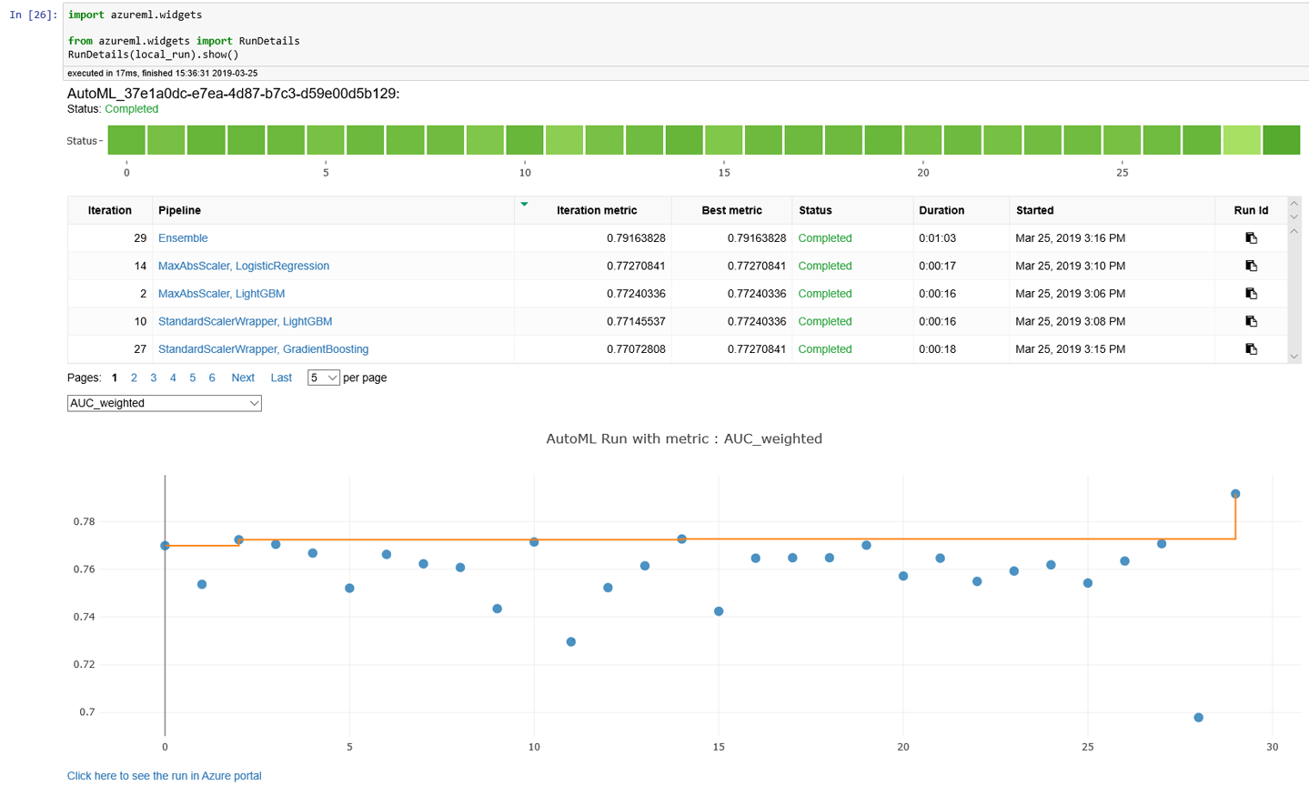
Figure 6-12. Using automated ML Jupyter Notebook widgets

A subset of this view is shown in Figure 6-13.

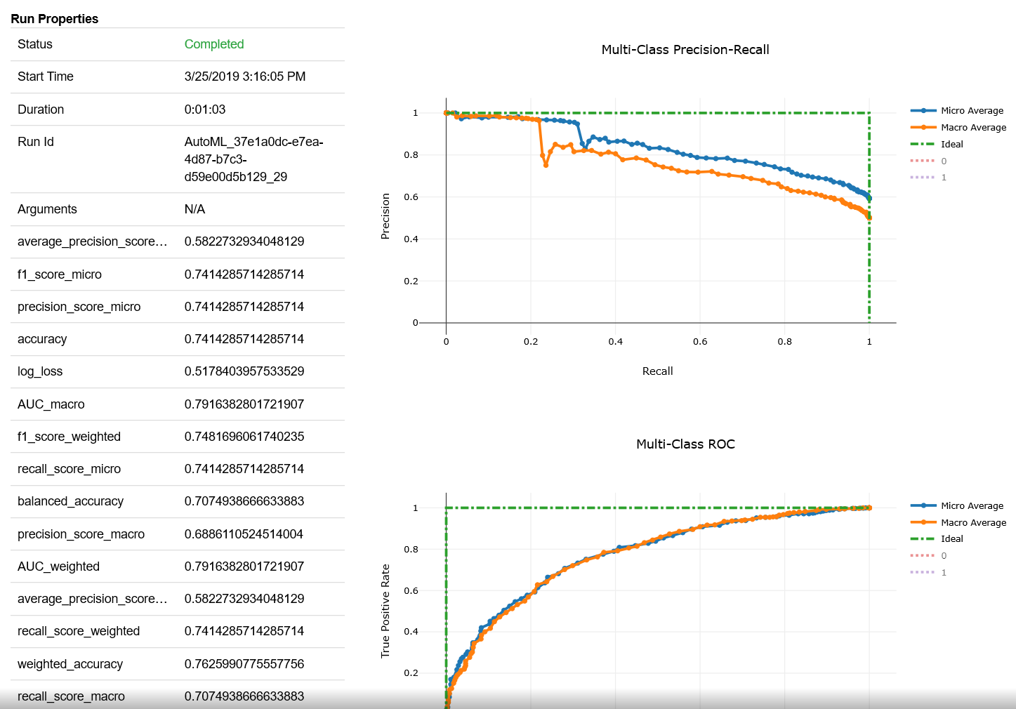
Figure 6-13. Using the automated ML Jupyter Notebook widgets to understand details about the run

Instead of interactively clicking each iteration, you can tabulate the metrics for each iteration in a run by using get_children() (the output is shown in Figure 6-14):

# Get all child runs
children = list(local_run.get_children())
metricslist = {}
for run in children:
    properties = run.get_properties()
    metrics = {k: v for k,
      v in run.get_metrics().items() if isinstance(v, float)}
    metricslist[int(properties['iteration'])] = metrics
rundata = pd.DataFrame(metricslist).sort_index(1)
rundata

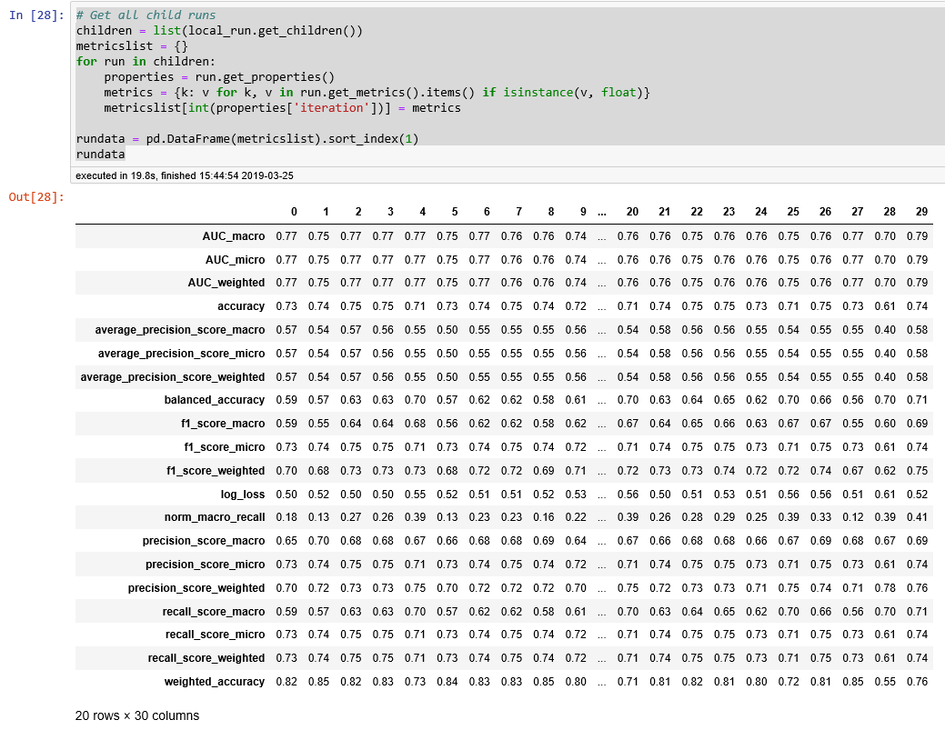
Figure 6-14. Metrics for each iteration in a run

Selecting and testing the best model from the experiment run

To use the best model, you can use the get_output() function (the output is shown in Figure 6-15):

best_run, fitted_model = local_run.get_output(metric = "AUC_weighted")

print(best_run)

Figure 6-15. Information about the best run

Let’s test the model using the test data, and understand the classification metrics from the evaluation, as well as the area under the receiver operating characteristic curve (ROC AUC):

from sklearn.metrics import classification_report
from sklearn.metrics import roc_auc_score

y_pred = fitted_model.predict(X_test)

target_names = ['0','1']
print (classification_report(
          y_test,y_pred, target_names=target_names))
print("AUC: " + str(roc_auc_score(y_test,y_pred)))

Figure 6-16 shows the output from testing the model using the test data, and the relevant metrics: precision, recall, f1-score, and support for the model.

Figure 6-16. Classification metrics and AUC for the best model selected

Conclusion

In this chapter, you learned how to use automated ML with Azure Machine Learning to find the best classification models for predicting a person’s credit risk. You can also use the same approach for identifying the best regression models. After you’ve identified the best classification/regression models for a task, refer to Chapter 5 to see how to deploy the machine learning models to various environments.