Scapy is a Python program written to manipulate network packets. It differs from most other tools because it is not a shell command program but comes in the shape of an interpreter. Actually, Scapy uses the Python interpreter evaluation loop to let you manipulate classes, instances, and functions.
Scapy comes with some new concepts and paradigms that make it a bit different from other tools in the domain of networking tools. With Scapy, packets are materialized in the shape of class instances. Creating a packet means instantiating an object, and manipulating a packet means changing attributes or calling methods of this instance object.
The basic building block of a packet is a layer, and a whole packet is built by stacking layers on top of one another. For example, a DNS packet captured on an Ethernet link will be seen as a DNS layer stacked over a UDP layer, stacked over an IP layer, stacked over an Ethernet layer. Because of this layering, using objects allows for an almost natural representation and code implementation. By implementing packets as objects, creating a packet from scratch is done in one line of code while it would have taken many lines in C, even with the best libraries. This allows for ease of use, and the user can implement and experiment with theoretical attacks much faster.
Moreover, the logic of sending packets, sniffing packets, matching a query and a reply, presenting couples, and tables is always the same and is provided by Scapy. A new tool can be designed in three steps:
Create your set of packets.
Call Scapy's logic to send them, gather the replies, parse them, match stimuli and answers.
Display the result.
A tool that says "I have received a TCP Reset packet from port 80" is decoding the packet it has received and is rewriting it in something human beings understand more easily. A tool that says "The port 80 is closed" is trying to interpret the reply packet with the logic it was given by its author. But you are doing the pen test, not the tool's author, and now you have to trust digital translation of the author's analysis logic, which may have been poorly implemented in the tool.[26] How could the author have known, at the time of writing the tool, all the complicated situations in which it would be used and trusted?
Choosing the right tool can be crucial to having accurate results, and having accurate results can save you time. For example, consider a situation where you are scanning a network that is 15 hops away. Receiving a TCP reset packet from port 80 surely means no service is reachable there. Most tools will report the port as being closed. What if in a parallel world, an alternative "you" uses a tool that reports a reset packet from port 80 with TTL 242, while other packets on other ports came with TTL 241. The other "you" would know that the reset packet is spoofed by the router before the scanned box and that the packet never reached the box itself. You could spend hours understanding why your backdoor cannot take the place of this closed port, while your alternate being uses another port, finishes his pen test report early, and spends the rest of the week on the beach having a good time.
Here is another example of a tool interpreting a situation:
# nmap 192.168.9.3
Interesting ports on 192.168.9.3:
PORT   STATE    SERVICE
22/tcp filtered ssh
Nmap says that the port is filtered, but this answer has been triggered by a host unreachable ICMP error sent by the last router. In this context, the ICMP message has been interpreted as The packet has been blocked on its way to the target, while it should have been interpreted as The packet was to be delivered, but the target was not reachable. This situation typically occurs when a port is allowed to pass on a whole IP network block while not all IP addresses are used. This is a gold mine of information when you want to set up a backdoor, but if you trust your tool, not only will you miss the gold, but you'll also lose the whole mine because Nmap makes you wrongly assume no backdoor can be implanted there.
Trying to program analysis logic into a tool is a common error. If a tool is not designed as an expert system, program it as a tool, not as an expert.
Similar problems arise from tools that only partially decode what they receive. Choosing what to show and what to hide is a form of interpretation because the author decided for you what was interesting and what was not. While this may be valid 99 percent of the time, you may not notice on the occasion it is not valid and miss something important in an audit. Such programs always miss the unexpected, by definition. Too bad the unexpected things are often the most interesting. For instance, if we look at Example 6-1, we see nothing interesting.
Example 6-1. hping partial decoding
# hping -c 1 --icmp 192.168.8.1

HPING 192.168.8.1 (eth0 192.168.8.1): icmp mode set, 28 headers + 0 data bytes

len=46 ip=192.168.8.1 ttl=64 id=62361 icmp_seq=0 rtt=9.0 ms


--- 192.168.8.1 hping statistic ---

1 packets transmitted, 1 packets received, 0% packet loss

round-trip min/avg/max = 9.0/9.0/9.0 ms
But if we look carefully at what is really happening, as shown in the tcpdump output in Example 6-2, we may notice that the Ethernet padding ends with four nonnull bytes. This may indicate the presence of an Etherleak flaw. We would need to investigate further to confirm that, but we would have missed it with only hping.
Example 6-2. tcpdump output
13:50:37.081804 IP 192.168.8.1 > 192.168.8.14: ICMP echo reply, id 36469, seq 0, lengt
h 8

0x0000:  4500 001c f399 0000 4001 f5e7 c0a8 0801  E.......@.......

0x0010:  c0a8 080e 0000 718a 8e75 0000 0000 0000  ......q..u......

0x0020:  0000 0000 0000 0000 0000 443f a2d0       ..........D?.
Compared to machines, human beings are quite bad at decoding binary stuff and often have to seek help in this domain. On the other hand, machines are quite bad at interpreting stuff, and it should be left up to humans to draw the conclusions.
Scapy dissociates the information harvesting phase and the result analysis. For example, you have to send a specific set of packets when you want to do a test, a port scan, or a traceroute. The packets you get back contain more information than just the simple result of the test and may be used for other purposes. Scapy returns the whole capture of the sent and received packets, matched by stimulus-response couples. You can then analyze it offline, as many times as you want, without probing again. This reduces the amount of network traffic and exposure to being noticed or flagging some IDS.
This raw result is decoded by Scapy and usually contains too much information for a human being to interpret anything right away. In order to make sense of the data, you will need to choose an initial view of interpretation where a meaning may become obvious.
The drawback of this that it requires many more resources than only keeping what is useful for the current interpretation. However, it can save time and effort afterwards. Also, refining an interpretation without a new probe is more accurate because you can guarantee that the observed object did not change between probes. Always working on the same probe's data guarantees consistency of observations.
While Scapy has numerous features, it does come with some quirks that the user should be aware of. The first is that Scapy is not designed for fast throughput. It is written in Python, has many layers of abstraction, and it is not very fast. Do not expect a packet rate higher than 6 Mbs per second. Because of these layers of abstraction, and because of being written in Python, it may also require a lot of memory. When dealing with large amounts of packets, packet manipulation becomes uncomfortable after about 216 packets.
Scapy is stimulus-response-oriented. While you could do it, handling stream protocols may become painful. This is clearly an area of improvement. Yet, for the moment, it is possible to play with a datagram-oriented protocol over a stream socket managed by the kernel.
You can easily design something that sniffs, mangles, and sends. This is exactly what is needed for some attacks. But you will be disappointed in terms of performance or efficiency if you expect Scapy to do the job of a router. Do not confuse Scapy with a production mangling router that you could obtain with Netfilter.
Scapy is not a traditional shell command-line application. When you run it, it will provide you with a textual environment to manipulate packets. Actually, it will run the Python interpreter and provide you many objects and functions that will enable you to manipulate packets.
Tip
If you are not familiar with Python programming, you can examine some of the Python tutorials located at www.python.org. The Python language offers fantastic flexibility and ease of use, and is object oriented. The tutorial should take between 30 minutes and 2 hours to complete, depending on your programming background.
Python has been designed to teach computer programming. If you have never programmed at all, do not be afraid to jump aboard. There are many resources available to help you learn both programming and Python at the same time. I suggest running Scapy while reading the sections and play along with the examples.
Scapy runs in a Python interpreter; because of this, you can leverage the full functionality of Python. This means that you will be able to use Python commands, loops, and the whole language when dealing with packets; for example:
#scapyWelcome to Scapy (1.0.4.55) >>>7*642 >>>[2*k for k in range(10)][0, 2, 4, 6, 8, 10, 12, 14, 16, 18]
Scapy adds some commands and classes through the built-ins. For example, a call to the ls( ) function will list all the protocol layers supported by Scapy:
>>> ls(  )
ARP        : ARP
BOOTP      : BOOTP
DNS        : DNS
Dot11      : 802.11
[...]
You can also use ls( ) to list the fields of a given layer. In the dump listed next, the first column contains the names of the fields in the packet. The second column is the name of the class used to manage the field's value. The last column displays the default value of the field. None is the special Python object that means that no value has been set and that one will be computed at packet assembly time. This is an important detail: the None object is not part of the set of possible values for the field, so that no value is sacrificed to have this special meaning.
>>>ls(IP)version : BitField = (4) ihl : BitField = (None) tos : XByteField = (0) len : ShortField = (None) id : ShortField = (1) flags : FlagsField = (0) frag : BitField = (0) ttl : ByteField = (64) proto : ByteEnumField = (0) chksum : XShortField = (None) src : Emph = (None) dst : Emph = ('127.0.0.1') options : IPoptionsField = ('') >>>ls(TCP)sport : ShortEnumField = (20) dport : ShortEnumField = (80) seq : IntField = (0) ack : IntField = (0) dataofs : BitField = (None) reserved : BitField = (0) flags : FlagsField = (2) window : ShortField = (8192) chksum : XShortField = (None) urgptr : ShortField = (0) options : TCPOptionsField = ({})
A network packet is divided into layers, and each layer is represented by a Python instance. Thus manipulating a network packet is done by playing with instances' attributes and methods representing the different layers of the packet. Creating a packet is done by creating instances, one for each layer, and stacking them together. For example, let's create a TCP/IP packet to port 22:
>>>a=IP( )❶ >>>a<IP |> >>>a.ttl❷ 64 >>>a.ttl=32❸ >>>a<IP ttl=32 |> >>>b=TCP(dport=22)❹ >>>c=a/b❺ >>>c<IP frag=0 ttl=32 proto=TCP |<TCP dport=ssh |>> >>>c.proto6 ❻
First, ❶ create an IP instance and store it into variable a. All the IP fields are set to their respective default value—the one that can be seen with ls( ). Access the fields: they appear as attributes of the instance. ❷ Ask for the TTL value, which is 64 by default. ❸ Set it to 32. The representation of the packet shows that the TTL field does not have its default value anymore. Then, ❹ create a TCP layer. Set some fields' values directly at instance construction. Then, ❺ stack a and b using the / operator to create a TCP/IP packet. Notice that some IP fields have their value automatically set to a more useful one. ❻ The IP protocol field value has been overloaded by the TCP layer to be IPPROTO_TCP (i.e., 6).
As we can see in Figure 6-1, each layer can hold three values for each field. The first one, always present, is the default value. The second one can be set by an upper layer that would overload some default values (as TCP did previously for the IP protocol field). The third one is the one set by user, and overloads the previous ones.
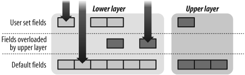
We have used ls( ) to show information about a layer, which is also a class, but it also works for instances of an object. A new column has appeared before the default values and gives the current value. This column takes into account what the user set and what other layers may have overloaded.
>>> ls(c)
version    : BitField             = 4               (4)
ihl        : BitField             = None            (None)
tos        : XByteField           = 0               (0)
len        : ShortField           = None            (None)
id         : ShortField           = 1               (1)
flags      : FlagsField           = 0               (0)
frag       : BitField             = 0               (0)
ttl        : ByteField            = 32              (64)
proto      : ByteEnumField        = 6               (0)
chksum     : XShortField          = None            (None)
src        : Emph                 = '127.0.0.1'     (None)
dst        : Emph                 = '127.0.0.1'     ('127.0.0.1')
options    : IPoptionsField       = ''              ('')
--
sport      : ShortEnumField       = 20              (20)
dport      : ShortEnumField       = 22              (80)
seq        : IntField             = 0               (0)
ack        : IntField             = 0               (0)
dataofs    : BitField             = None            (None)
reserved   : BitField             = 0               (0)
flags      : FlagsField           = 2               (2)
window     : ShortField           = 8192            (8192)
chksum     : XShortField          = None            (None)
urgptr     : ShortField           = 0               (0)
options    : TCPOptionsField      = {}              ({})
Fields can be assigned a wrong or cranky value. This is ideal to test network stack robustness and the ability to handle the unexpected.
>>> IP(version=2, ihl=3, options="love", proto=1)/TCP(  )
<IP  version=2 ihl=3 frag=0 proto=ICMP options='love' |<TCP  |>>
Fields can also be assigned a set of values. This is perfect to quickly create a set of packets from a given template, and more particularly to go through many values of a given field (a.k.a. scanning). Packets whose one or more fields contain a set of values will be called implicit packets.
>>>pkts = IP(ttl=[1,3,5,(7,10)])/TCP( )❶ >>>pkts<IP frag=0 ttl=[1, 3, 5, (7, 10)] proto=TCP |<TCP |>> >>>[pkt for pkt in pkts][<IP frag=0 ttl=1 proto=TCP |<TCP |>>, <IP frag=0 ttl=3 proto=TCP |<TCP |>>, <IP frag=0 ttl=5 proto=TCP |<TCP |>>, <IP frag=0 ttl=7 proto=TCP |<TCP |>>, <IP frag=0 ttl=8 proto=TCP |<TCP |>>, <IP frag=0 ttl=9 proto=TCP |<TCP |>>, <IP frag=0 ttl=10 proto=TCP |<TCP |>>] >>>IP(dst="192.168.*.1-10")/ICMP( )❷ <IP frag=0 proto=ICMP dst=<Net 192.168.0-2.*> |<ICMP |>> >>>IP(dst="192.168.4.0/24")/TCP(dport=(0,1024))❸ <IP frag=0 proto=TCP dst=<Net 192.168.4.0/24> |<TCP dport=(0, 1024) |>>
Here we have created three implicit packets. ❶ The first one is worth seven TCP/IP packets with TTL 1, 3, 5, 7, 8, 9, and 10. This is a partial TCP traceroute. ❷ The second one will do an ICMP ping scan, going through the first 10 IP addresses of all the 192.168 networks. ❸ The third one will do a TCP SYN scan on all privileged ports of the 192.168.4.0/24 network.
As you can see, scanning doesn't just mean TCP port scanning. It means taking a field and going through all possible, or interesting, values. According to the fields you choose to scan, you will get a different tool. If you choose TCP destination ports, you will have all kinds of TCP port scanners, depending on which flags you choose to send. If you fix an interesting TTL at the same time, it becomes a firewalker (this network reconnaissance technique will be explained in Packet-Crafting Examples with Scapy). If you choose to scan destination IP, depending on whether you go for ICMP, TCP, or ARP, you will have a TCP ping, ICMP ping, or ARP ping IP scanner. If you choose to scan the TTL, you will have a traceroute tool. If your payload is a DNS or IKE request, and you scan the IP destination, you will scan the Internet for DNS servers or VPN concentrators. If you choose one DNS server and you scan through IP with reverse DNS request, you will have a reverse DNS bruteforcer. You are only limited by your imagination (or the limits discussed in Chapter 1).
When two or more layers are stacked one top of the other, you keep only a reference to the first one. A special attribute named payload is used to reference the next layer, and so on until the last layer, whose payload attribute points to a special stub: an instance of the NoPayload class.
>>>a=Ether()/IP()/TCP( )>>>a<Ether type=IPv4 |<IP frag=0 proto=TCP |<TCP |>>> >>>a.payload<IP frag=0 proto=TCP |<TCP |>> >>>a.payload.payload<TCP |>
When asking for a field value, if the attribute is not found in the current layer, it will be looked for recursively in upper layers.
Warning
This is not true when setting a value to an attribute. If the attribute does not exit in the current layer, it will be created and will even take precedence over a potential field in upper layers.
>>>a.type2048 >>>a.proto6 >>>a.dst'ff:ff:ff:ff:ff:ff' >>>a.payload.dst'127.0.0.1'
Warning
Pay attention to the fact that some layers may have the same field names and that one may be found before the one you thought about. This is especially true for Ether and IP (which both have src and dst fields), and also for IP and TCP (which both have flags fields).
Accessing and manipulating layers using the payload special attribute is generally not practical. It is usually better to use an absolute way to address a layer in the packet by its class name:
>>>a[IP]<IP frag=0 proto=TCP |<TCP |>> >>>a[TCP]<TCP |> >>>a[IP].dst'127.0.0.1'
Tip
This way of addressing has many advantages, and it is in particular totally independent of lower layers. For instance, if you want to work on DNS layers of a set of packets, asking for the DNS layer will work whether you are sniffing on a PPP link, on a 802.11 link in monitor mode, or on a GRE tunnel.
If a layer is not present in a packet, None will be returned. If you try to do something on a layer that is not present, you will surely get an error. To test for the presence of a given layer in a packet, you can use the needle in haystack idiom:
>>>IP in aTrue >>>ISAKMP in aFalse
Scapy has numerous options and capabilities. To make full use of Scapy, users should familiarize themselves with the many options detailed in the online manual. However, here are some shortcut examples of how to use Scapy to get things done.
Use hide_defaults( ) to remove any user-supplied value that is identical to the default value. This is very useful after a dissection, where all the user fields are set and thus displayed.
>>>a=IP()/TCP( )>>>b=IP(str(a))>>>b<IP version=4L ihl=5L tos=0x0 len=40 id=1 flags= frag=0L ttl=64 proto=TCP chksum=0x7ccd src=127.0.0.1 dst=127.0.0.1 options='' |<TCP sport=ftp-data dport=www seq=0L ack=0L dataofs=5L reserved=0L flags=S window=8192 chksum=0x917c urgptr=0 |>> >>>b.hide_defaults( )>>>b<IP ihl=5L len=40 frag=0 proto=TCP chksum=0x7ccd src=127.0.0.1 |<TCP dataofs=5L chksum=0x917c |>>
The show( ) will output a detailed dissection of a packet. But some automatically computed fields (e.g., checksums) cannot be computed without assembling the packet. If you want to know those values, show2( ) will completely assemble the packet and disassemble it again to take into account all the post build operations such as lengths or checksum computations. For instance, look at the ihl ❶ and chksum ❷ fields in the following example:
>>>IP().show( )>>>IP().show2( )###[ IP ]### ###[ IP ]### version= 4 version= 4 ihl= 0 ❶ ihl= 5 ❶ tos= 0x0 tos= 0x0 len= 0 len= 20 id= 1 id= 1 flags= flags= frag= 0 frag= 0 ttl= 64 ttl= 64 proto= IP proto= IP chksum= 0x0 ❷ chksum= 0x7ce7 ❷ src= 127.0.0.1 src= 127.0.0.1 dst= 127.0.0.1 dst= 127.0.0.1 options= '' options= ''
Use decode_payload_as( ) to change the way a payload is decoded. Here we change the Raw layer❶ into an IP layer ❷:
>>>pkt=str(IP( )/UDP(sport=1,dport=1)/IP(dst="1.2.3.4"))>>>a=IP(pkt)>>>a<IP version=4L ihl=5L tos=0x0 len=48 id=1 flags= frag=0L ttl=64 proto=UDP chksum=0x7cba src=127.0.0.1 dst=127.0.0.1 options='' |<UDP sport=1 dport=1 len=28 chksum=0x1b2 |<Raw (1)[CALLOUT] load="E\x00\x00\x14\x00\x01\x00\x00@\x00\xb1'\xc0 \xa8\x05\x14\x01\x02\x03\x04" |>>> >>>a[UDP].decode_payload_as(IP)>>>a<IP version=4L ihl=5L tos=0x0 len=48 id=1 flags= frag=0L ttl=64 proto=UDP chksum=0x7cba src=127.0.0.1 dst=127.0.0.1 options='' |<UDP sport=1 dport=1 len=28 chksum=0x1b2 |<IP (2)[CALLOUT] version=4L ihl=5L tos=0x0 len=20 id=1 flags= frag=0L ttl=64 proto=IP chksum=0xb127 src=192.168.5.20 dst=1.2.3.4 |>>>
The sprintf( ) method is one of the key methods that will help you with writing most tools in only two lines. It will fill a format string with values from the packet, a bit like the sprintf( ) function from the C library. However, the format directives refer to layer names and field names instead of arguments in a list. If a layer or a field is not found, the ?? string is displayed instead.
>>>a.sprintf("Ethernet source is %Ether.src% and IP proto is %IP.proto%")'Ethernet source is 00:00:00:00:00:00 and IP proto is TCP' >>>a.sprintf("%Dot11.addr1% or %IP.gabuzomeu%")'?? or ??'
The exact format of a directive is:%[[fmt][r],][layer[:nb].]field%
layerThe name of the layer from which you want to take the field. If it is not present, the current layer is used.
fieldThe name of the field you want the value of.
nbWhen there are many layers with the same name—for instance, for an IP over IP packet—
nbis used to reach the one of your choice.rris a flag. When present, it means you want to work on the raw value of the field. For example, a TCP flags field can be represented as the human readable stringSAto indicate the flags SYN and ACK are set. Its raw value is the number 18.fmtfmtis used to give formatting directives à laprintf( )to be applied to the value of the field.
Here are some examples to illustrate this:
>>>a=Ether( )/Dot1Q(vlan=42)/IP(dst="192.168.0.1")/TCP(flags="SA")>>>a.sprintf("%dst% %IP.dst% vlan=%Dot1Q.vlan%")'00:00:d4:ae:3f:71 192.168.0.1 vlan=42' >>>a.sprintf("%TCP.flags%|%-5s,TCP.flags%|%#05xr,TCP.flags%")'SA|SA |0x012' >>>b=Ether()/IP(id=111)/IP(id=222)/UDP( )/IP(id=333)>>>b.sprintf("%IP.id% %IP:1.id% %IP:2.id% %IP:3.id%")'111 111 222 333'
This same technique can be used to perform similar operands on many packets and allow you to treat them all differently:
>>>f=lambda x:x.sprintf("%IP.dst%:%TCP.dport%")>>>f(IP()/TCP( ))'127.0.0.1:www' >>>f(IP()/UDP( ))'127.0.0.1:??' >>>f(IP()/ICMP( ))'127.0.0.1:??'
As you can see, I defined a lambda function f that is supposed to be applied to different packets, but can only handle TCP packets. It would not be very practical to define a real function with a case disjunction to treat all possible cases. That is why I have integrated conditional substrings into sprintf( ). A conditional substring looks like {[!]layer:substring}. When layer is present in the packet, the conditional substring is replaced with substring. Else it is simply removed. If ! is present, the condition is inversed.
>>>f=lambda x: x.sprintf("=> {IP:ip=%IP.dst% {UDP:dport=%UDP.dport%}\{TCP:%TCP.dport%/%TCP.flags%}{ICMP:type=%r,ICMP.type%}}\{!IP:not an IP packet}")>>>f(IP()/TCP( ))'=> ip=127.0.0.1 www/S' >>>f(IP()/UDP( ))'=> ip=127.0.0.1 dport=domain' >>>f(IP()/ICMP( ))'=> ip=127.0.0.1 type=8' >>>f(Ether()/ARP( ))'=> not an IP packet'
Here, the same lambda function can be applied to any packet and will adapt what to display according to the packet it is applied to.
Many times you will not work on just one packet but on a set of packets. That is why special objects have been designed to hold lists of packets and to provide methods to manipulate and visualize those lists easily.
Lists can come into many flavors. The basic kind is the PacketList. It can hold a list of any packets. It has a variant, the Dot11PacketList, which adds special functionalities for 802.11 packets, such as counting the number of beacons or providing an additional method to convert the whole list of 802.11 packets into Ethernet packets. PacketList is also derivated into SndRcvList, which mainly differs by the fact it does not hold a list of packets but a list of couples of packets. This kind of list is used when you do a network probe. As we have seen, Scapy returns the raw result of the probe. This comes in the shape of a list of couples in a SndRcvList instance. Each couple is made of the stimulus packet and the response packet. SndRcvList is in turn derivated into other flavors such as TracerouteResult, whose goal is to hold the raw result of a specific kind of probe. They provide special methods to visualize or study those raw results:
>>>a=sniff(count=10)>>>a<Sniffed: UDP:0 TCP:7 ICMP:0 Other:3> >>>b=Dot11PacketList(a)>>>b<Dot11List: ICMP:0 802.11 Beacon:2 802.11 WEP packet:0 UDP:0 TCP:7 Other:1> >>>traceroute("www.slashdot.net")[...] (<Traceroute: UDP:0 TCP:8 ICMP:17 Other:0>, <Unanswered: UDP:0 TCP:5 ICMP:0 Other:0>)
Packet lists are, before all, lists. You can do to packet lists what you can do to lists. You can access a given item, take a slice out, or sort them:
>>>a[3:5]<mod Sniffed: UDP:0 TCP:2 ICMP:0 Other:0> >>>a+b<Sniffed+Dot11List: UDP:0 TCP:20 ICMP:0 Other:0>
Some additional operations have been added; e.g., you can filter for packets of a given type:
>>> a[TCP]
<TCP from Sniffed: UDP:0 TCP:7 ICMP:0 Other:0>The conversations( ) method will create a conversation graph such as the one shown in Figure 6-2. It requires graphviz and ImageMagick to work.
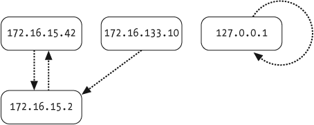
>>> a.conversations( )You are not limited to conversations at the IP level. You can provide a function that returns the source and destination of any item. By default, the lambda x: (x[IP].src, x[IP].dst) function is used, but you could use lambda x:(x.src,x.dst) to work at the Ethernet level.
Emitting packets on the wire is done either at layer 3 with send( ) or at layer 2 with sendp( ). send( ) will route the packet, choose the layer 2 according to the output interface, and fill it with the right values. For instance, it will do an ARP request to get the MAC address of the gateway if necessary. sendp( ) will use the default output interface (conf.iface). You can force the use of a given interface with the iface parameter. Alternatively, the hint_iface parameter can be assigned an IP and the interface will be chosen with a lookup into the routing table. When the loop parameter is nonnull, the packets are sent until Ctrl-C is pressed. The inter parameter can be assigned a time in seconds to wait between each packet.
The send and receive functions family will not only send stimuli and sniff responses but also match sent stimuli with received responses. Functions sr( ), sr1( ), and srloop( ) all work at layer 3. While sr( ) returns the whole result of a probe, i.e., a SndRcvList of stimulus-response couple and a PacketList of unreplied stimuli, sr1( ) returns only the first reply to a stimulus. Function srloop( ) will send some stimuli repeatedly and print a summary of the result of each probe. Its return value is the same as sr( ), but for all the probes together. The functions srp( ), srp1, and srploop( ) work at layer 2 and do exactly the same as their layer 3 counterparts.
The layer 2 and layer 3 sr*( ) functions all share the same base parameters: timeout, retry, inter, iface, filter, and multi.
timeout can be assigned a time in seconds after which Scapy can stop waiting for answers. The timer starts right after the last packet is sent. Thus, the timeout depends only on the network latency, not on the number of stimuli sent.
retry is maybe the most complex parameter here. It determines the management of unanswered stimuli. By default, nothing is done. If a positive value is set, it fixes the maximum number of times a stimulus can be sent. Stimuli that are unanswered after the first round will be sent again in another round, and again and again until they are answered or the number of sendings reaches the value of retry. The timeout parameter is used at each round. By default, there is no timeout so you will have to press Ctrl-C at each round. A better behavior is possible with negative values of retry. Their absolute value determines how many times in a row a round must have no replies at all before stopping. This means that as long as we get new replies, we will run other rounds, and we need to have -retry empty rounds before stopping.
Tip
If explanations about retry are too complicated, just remember that retry=-2 is a good value suitable for most situations.
inter can be assigned a time in seconds to wait between two sendings.
Tip
Many equipment use rate limits on ICMP packets. While you can have all your stimuli answered one by one with a negative retry value, you can reach the same result with less bandwidth by using a well-chosen inter value.
The iface parameter can force the sr*( ) functions to listen for replies on a provided interface, rather than listening on all interfaces by default.
The filter parameter can be assigned a BPF filter to limit what Scapy sees on the network. If you are on a very crowded network, Scapy may not be able to keep the pace and may lose packets or at least take time to decode everything before reaching the awaited answers. If you know the kind of answers you are expecting, use filter to drop unwanted packets as early as possible and save a lot of CPU time.
Setting multi parameter to a nonnull value will enable multiple-answer mode. In normal mode, once a stimulus has been answered, Scapy will remove it from the list of stimuli awaiting an answer. In the former mode, if a stimulus triggers many answers—a broadcast ping, for instance—each answer will be recorded in the stimulus-response list. Thus, the same stimulus may appear many times in the list, coupled to different responses.
Let's say we want to do the most classical thing a network tool would do: a TCP SYN scan. We need to send TCP SYN packets to a target by going through interesting TCP ports. We will focus on privileged TCP ports and ports 3128 and 8080:
>>> sr(IP(dst="192.168.5.1")/TCP(dport=[(1,1024),3128,8080]))
Begin emission:
.**..
Received 4 packets, got 2 answers, remaining 1024 packets
(<Results: UDP:0 ICMP:0 TCP:2 Other:0>, <Unanswered: UDP:0 ICMP:0 TCP:1024 Other:0>)
>>> res,unans=_
>>> res.nsummary(  )
0000 IP / TCP 192.168.5.20:ftp-data > 192.168.5.1:ssh S ==>
                           IP / TCP 192.168.5.1:ssh > 192.168.5.20:ftp-data SA
0001 IP / TCP 192.168.5.20:ftp-data > 192.168.5.1:www S ==>
                           IP / TCP 192.168.5.1:www > 192.168.5.20:ftp-data SA
We got only two positive responses, so it is very likely that the target runs a firewall that dropped all but the connections to the SSH and web port:
>>> sr(IP(dst="192.168.5.22")/TCP(dport=[(1,1024),3128,8080]))
Begin emission:
.******************************************[...]Finished to send 1026 packets.
*
Received 1036 packets, got 1026 answers, remaining 0 packets
(<Results: UDP:0 ICMP:0 TCP:1026 Other:0>, <Unanswered: UDP:0 ICMP:0 TCP:0 Other:0>)
>>> res,unans = _
>>> res.nsummary(  )
0000 IP / TCP 192.168.5.20:ftp-data > 192.168.5.22:tcpmux S ==>
             IP / TCP 192.168.5.22:tcpmux > 192.168.5.20:ftp-data RA / Padding
0001 IP / TCP 192.168.5.20:ftp-data > 192.168.5.22:2 S ==>
                  IP / TCP 192.168.5.22:2 > 192.168.5.20:ftp-data RA / Padding
[...]
This time we have many more answers, but some are negative. Indeed nothing dropped our packets, and the target's OS sent us RST-ACK TCP packets when ports were closed. Analyzing the results with this output is not really practical. We can provide a filter function that will decide whether a couple should be displayed or not with the lfilter argument. In this case, the function will be a lambda function that takes a stimulus-response couple (s,r) and returns whether the response r has the TCP SYN flag or not:
>>> res.nsummary(lfilter = lambda (s,r): r[TCP].flags & 2)
0008 IP / TCP 192.168.5.20:ftp-data > 192.168.5.22:discard S ==>
            IP / TCP 192.168.5.22:discard > 192.168.5.20:ftp-data SA / Padding
0012 IP / TCP 192.168.5.20:ftp-data > 192.168.5.22:daytime S ==>
            IP / TCP 192.168.5.22:daytime > 192.168.5.20:ftp-data SA / Padding
0021 IP / TCP 192.168.5.20:ftp-data > 192.168.5.22:ssh S ==>
                IP / TCP 192.168.5.22:ssh > 192.168.5.20:ftp-data SA / Padding
0024 IP / TCP 192.168.5.20:ftp-data > 192.168.5.22:smtp S ==>
               IP / TCP 192.168.5.22:smtp > 192.168.5.20:ftp-data SA / Padding
If this is still not straightforward enough, we can also choose what to display by providing a function to the prn argument.
>>> res.nsummary(lfilter = lambda (s,r): r[TCP].flags & 2,
...              prn = lambda (s,r):s.dport)
0008 9
0012 13
0021 22
0024 25
0036 37
0138 139
0444 445
0514 515
This may seems strange at first, but retaining all of the probe's information to analyze it later enables you to look at it along a different axis of analysis. For example, you can see there is padding in response packets, so you can look for open TCP ports and then for information leaking into the padding or make a full TTL analysis. It also enables you to refine the visualization as much as you want.
As an illustration, can you tell the difference between Example 6-3 and Example 6-4? Do not spend too much time pondering it because there is no difference. You might be thinking the two probed networks are configured in the same fashion, but this is not the case. This time the tool is the limit. See Example 6-5 to view the difference. In one case the packet to port 79 has been dropped, and in the other, an ICMP destination unreachable/host prohibited has been sent.
This might seem like an insignificant detail, but when you try to remotely map a network, every detail is important. In this case, we know that our packets are answered, and we can use this to know exactly where packets are stopped. This is useful to know if we try negative scans such as UDP or IP protocol ones where a lack of answer is considered as a positive result. This also enables us to do a TTL analysis on our probe. The TTL from the ICMP error message we received was 240. It probably was 255 at its creation. The TTL of the TCP answer was 48, and it was probably the next power of 2 at its creation (i.e., 64). So, there is a difference of (64-48) - (255-240)=1 hop between the web server and the firewall, meaning the web server is very probably right behind the firewall.
Example 6-3. Sample scan 1
# nmap -p 79,80 www.slashdot.org

Starting Nmap 4.00 ( http://www.insecure.org/nmap/ ) at 2006-08-11 18:55 CEST
Interesting ports on star.slashdot.org (66.35.250.151):
PORT   STATE    SERVICE
79/tcp filtered finger
80/tcp open     http

Nmap finished: 1 IP address (1 host up) scanned in 5.406 seconds
Example 6-4. Sample scan 2
# nmap -p 79,80 www.google.com
Starting Nmap 4.00 ( http://www.insecure.org/nmap/ ) at 2006-08-11 18:55 CEST
Interesting ports on 66.249.91.99:
PORT   STATE    SERVICE
79/tcp filtered finger
80/tcp open     http
Nmap finished: 1 IP address (1 host up) scanned in 12.253 seconds
Example 6-5. Scan sample 3
>>> res1,unans1=sr(IP(dst="www.slashdot.org")/TCP(dport=[79,80]))
Begin emission:
.Finished to send 2 packets.
**
Received 3 packets, got 2 answers, remaining 0 packets
>>> res1.nsummary(  )
0000 IP / TCP 192.168.5.20:ftp-data > 66.35.250.151:finger S ==>
   IP / ICMP 66.35.250.151 > 192.168.5.20 dest-unreach 10 / IPerror / TCPerror
0001 IP / TCP 192.168.5.20:ftp-data > 66.35.250.151:www S ==>
                         IP / TCP 66.35.250.151:www > 192.168.5.20:ftp-data SA
>>> res2,unans2=sr(IP(dst="www.google.com")/TCP(dport=[79,80]))
Begin emission:
Finished to send 2 packets.
*
Received 1 packets, got 1 answers, remaining 1 packets
>>> res2.nsummary(  )
0000 IP / TCP 192.168.5.20:ftp-data > 64.233.183.104:www S ==>
IP / TCP 64.233.183.104:www > 192.168.5.20:ftp-data SATo read and write packets to the network, Scapy uses a super-socket abstraction. A super-socket is an object that provides operations to send and receive packets. It can rely on sockets or on libraries such as libpcap and libdnet. It manages BPF filtering and assembling and dissecting packets, so that you send and receive packet objects, not strings. Some super-sockets offer layer 2 access to the network and others layer 3 access. The latter will manage the routing table lookup and choose a suitable layer 2 according to the output interface. Both will choose the layer class to instantiate when receiving a packet according to the interface link type.
L2Socket and L3PacketSocket are the default for Linux. They use the PF_PACKET protocol family sockets. On other Unixes, L2dnetSocket and L3dnetSocket are used. They rely on libpcap and libdnet to send and receive packets. The super-sockets to use are stored into conf.L2socket and conf.L3socket, so you could, for example, switch to use libpcap and libdnet even though you are on Linux. You could also write a new super-socket that could receive traffic remotely from a TCP tunnel. L2ListenSocket and L2pcapListenSocket are dumb super-sockets used only by sniff( ). The one to use is stored in conf.L2listen. Another layer 3 super-socket exists. It uses SOCK_RAW type of PF_INET protocol family socket, also known as raw sockets. These kind of sockets are much more kernel-assisted and work on most Unixes. But they are designed to help standard applications, not applications that try to send invalid traffic. Among other limitations, you will not be able to send an IP packet to a network address present in your routing tables or an IP checksum set to zero because the kernel would compute it for you.
Other super-sockets exist. For example, the Scapy Teredo extension comes with a Teredo super-socket that provides you with IPv6 access from almost any IPv4-only box.
If you try to have Scapy interact with programs through your loopback interface, it would probably not work. You will see the packets with tcpdump but the target program will not. That is because the loopback interface does not work like a physical one.
If you want this to work, you have to send your packets through the kernel using PF_INET/SOCK_RAW sockets; i.e., by using L3RawSocket instead of L3PacketSocket or L3dnetSocket:
>>> sr1(IP()/ICMP(  ), timeout=1)
Begin emission:
.Finished to send 1 packets.

Received 1 packets, got 0 answers, remaining 1 packets
As expected, there was no answer. You need to use L3RawSocket:
>>> conf.L3socket=L3RawSocket
>>> sr1(IP()/ICMP(  ), timeout=1)
Begin emission:
Finished to send 1 packets.
.*
Received 2 packets, got 1 answers, remaining 0 packets
<IP  version=4L ihl=5L tos=0x0 len=28 id=28449 flags=
 frag=0L ttl=64 proto=ICMP chksum=0xdbe src=127.0.0.1
 dst=127.0.0.1 options=''
|<ICMP  type=echo-reply code=0 chksum=0xffff id=0 seq=0 |>>
Super-sockets can be used directly to take advantage of the abstraction they provide that hides low-level details. You can either choose one directly or use those proposed by the conf object to also avoid choosing between native or libdnet/libpcap usage. Then, you can use send( ) and recv( ) methods to send and sniff. If you want to write new applications that need to interact with the network and that cannot use sniff( ) and send( ) functions for performance or elegance reasons, super-sockets are the way to go. For example:
>>> s=conf.L3socket(filter="icmp",iface="eth0")
>>> while 1:
...   p=s.recv(  )
...   s.send(IP(dst="relay")/GRE(  )/p[IP])
Now that we are familiar with Scapy's concepts and features, here is a recipe that can be used to write new tools or clone most other networking tools. Most other tools send many packets built on a given template, listen for answers, and display results. A TCP port scanner will send many TCP SYN packets to one or more targets on one or more TCP ports. This is the template and is what you have to build in Scapy. Sending it, listening for answers, and matching stimulus-response couples is already done by the sr*( ) functions. Then you obtain the stimulus-response couples list and the unanswered stimuli list. Most of the results can be displayed with a make_table( ) call. The sprintf( ) may also be very useful to create the content of the table's cells.
For example, we will try to write a TCP SYN scanner. A TCP SYN scan tool will show us which ports are open on which IP address. We know that we will need to create a set of TCP/IP packets and that their destination will be TARGET. We will scan ports from 0 to 1024, which are considered the privileged ports on a machine. The sending-receiving-matching job is done by sr( ) and will return the stimulus-response couples list and the unanswered packets list. Displaying this information is easily done with make_table( ). We will display a table with a target IP address as the column header, a target port as the row header, and the state of the port. When we receive a TCP packet, we will show the flags or an ICMP error along with the message and the ICMP type. Ports that were unanswered are ignored, but we could as well display something with the unans content:
>>> res,unans = sr(IP(dst=TARGET)/TCP(dport=(0,1024)), timeout=4, retry=-2)
>>> res.make_table(lambda (s,r):(s.dst, s.dport, r.sprintf("{TCP:%TCP.flags%}{ICMP:%IP
.src%#%r,ICMP.type%}")))
    42.39.250.148   42.39.250.150   42.39.250.151
22  SA              42.39.250.150#3 42.39.250.151#3
23  42.39.212.174#3 42.39.250.150#3 42.39.250.151#3
25  42.39.212.174#3 42.39.250.150#3 42.39.250.151#3
80  42.39.212.174#3 SA              SA
113 42.39.212.174#3 42.39.250.150#3 42.39.250.151#3
443 42.39.212.174#3 SA              SA
You can see a list of packets or couple of packets as a set of points in a multi-dimensional space. Each different field is a dimension. make_table( ) will project these points on a plane defined by two vectors and give the value of a third one. More prosaically, make_table( ) will take a function that, applied to an element of the list, will return a triplet. The triplet will contain what you want to see in the columns headers, what you want to see in the lines headers and what you want to put inside the table itself.
We can also display only positive answers (TCP has the SYN flag set). This time we put the ports horizontally and the IP address vertically. We display only an uppercase X in cells whose ports are open:
>>> res.filter(lambda (s,r):TCP in r and r[TCP].flags&2).make_table(lambda (s,r): \
                (s.dport, s.dst, "X"))
              22 80 443
42.39.250.148 X
42.39.250.150    X  X
42.39.250.151    X  X
Some firewalls drop TCP SYN packets that come without the TCP timestamp option. This can be achieved, for instance, with this Netfilter rule:
iptables -I INPUT -p tcp --syn --tcp-option ! 8 -j DROP
This will drop few legitimate clients, but it will make many TCP SYN scanners such as Nmap[27] totally blind. Indeed, when they build the SYN packet, these programs do not take time to add TCP options to optimize TCP transfers. They need only a quick answer. For example:
# nmap -sS 192.168.1.1

Starting nmap 3.75 ( http://www.insecure.org/nmap/ ) at 2007-01-11 10:52 CET
All 1663 scanned ports on 192.168.1.1 are: filtered
MAC Address: 00:13:10:10:33:a2 (Unknown)

Nmap run completed -- 1 IP address (1 host up) scanned in 35.398 seconds
# telnet 192.168.1.1 22
Trying 192.168.1.1...
Connected to 192.168.1.1.
Escape character is '^]'.
SSH-2.0-dropbear_0.47
With Nmap, you have no other choice than using a TCP connect scan because no parameter is present to add a TCP option in a SYN scan. With Scapy, we just have to add the option to our two-line scanner:
>>> res,unans = sr(IP(dst="192.168.8.1")/TCP(dport=(0,64)), timeout=4, retry=-2)
which becomes:
>>> res,unans = sr(IP(dst="192.168.8.1")/TCP(dport=(0,64),options=[('Timestamp',(0,0))
]),
                   timeout=4, retry=-2)
And the second line remains unchanged:
>>> res.filter(lambda (s,r):TCP in r and r[TCP].flags&2).make_table(lambda (s,r): \
                (s.dport, s.dst, "X"))
            22 53
192.168.8.1 X  X
To show how easy it is to build tools, consider this. Firewalking is a technique to map firewall rule-sets by scanning a target behind the firewall with fixed TTL. Depending on the topology and the firewall configuration of the analyzed network, one can see accepted connections even if they are dropped after the firewall, or see differences between internal IP addresses owned by the firewall and those owned by other machines. You can see one implementation in Example 6-6.
Example 6-6. A firewalker
res,unans = sr(IP(dst=TARGET, ttl=GW_TTL)/TCP(dport=(0,1024)), timeout=4)
res.make_table(lambda (s,r):(s.dst, s.dport, r.sprintf("{TCP:%TCP.flags%}     {ICMP:%I
P.src%#%r,ICMP.type%}")))
Another easy to build tool is a traceroute tool to aim at DNS servers by using a real DNS payload. With a simple UDP scan, reaching the target does not generate any reply. Here we trigger a reply when we reach the target and thus we can distinguish between a packet drop and a target hit. A possible implementation is shown in Example 6-7.
When a product uses a new or proprietary protocol, there may be no tool ready to help you assess its security. You may have to write a new tool from scratch in order to accomplish this task, but this usually takes a lot of time and effort. It is much more efficient if you have to focus only on re-implementing the protocol and use an existing framework that already provides everything to manipulate, visualize, send, receive, probe, fuzz, etc. Thankfully, Scapy's three-part architecture (the core, the protocols, and the techniques) provides just such a framework. This means that each time that something is added to the core, all the protocols will be able to take advantage of it. Each time a new protocol is added, all the core functionalities of Scapy are already there to enhance it. Thus, Scapy offers an efficient framework to describe new protocol layers.
A layer is compounded of a list of fields. Each field is described with an instance of a Field class or subclass. Each field has a name, a default value, and some other parameters depending upon its type.
As shown in Example 6-8, there are basic rules to make a new layer. Your new layer must be a subclass of Packet. The attribute name is used to hold the long name of the layer, the short one being the name of the class. Then, the list of fields is put into the fields_desc attribute. Here we have a 1-byte field named mickey, a short field (2 bytes) named minnie and an int field (4 bytes) named donald. They both are unsigned and big endian—the network endianness. The ShortField is the vanilla short field type. XShortField is a different flavor and expresses the fact that the preferred field's value representation is in hexadecimal notation. The IntEnumField is a flavor of IntField that can translate some values into identifiers and vice versa, according to a provided dictionary.
Tip
If you want to begin to play with new protocols right now, read "Writing Add-Ons" in Scapy before directly modifying the Scapy source.
Example 6-8. Creating a new field in Scapy
class MyField(Packet):
    name = "My Field"
    fields_desc = [ ByteField("mickey", 4),
                    XShortField("minnie", 67),
                    IntEnumField("donald", 2,
                                 {1:"happy", 2:"bashful", 3:"sneezy"})
                  ]
The simple description in Example 6-8 is sufficient to assemble, disassemble, and manipulate the layer like any other layer in Scapy. For example:
>>> a=MyField(mickey=2)
>>> a
<MyField  mickey=2 |>
>>> a.donald
2
>>> a.show(  )
###[ My Field ]###
  mickey= 2
  minnie= 0x43
  donald= bashful
>>> a.donald="happy"
>>> a.donald
1
>>> str(a)
'\x02\x00C\x00\x00\x00\x01'
>>> MyField(_)
<MyField  mickey=2 minnie=0x43 donald=happy |>
>>> send(IP(proto=42)/MyField(minnie=1))
.
Sent 1 packets.
This is possible because all the brainpower is concentrated into the fields classes. Several kinds of fields are provided.
As an example of concentrating the power into the fields classes, Figure 6-3 has a layer with a byte value that encodes a type, a field that encodes the length of a string, a flags field, four reserved unused bits, and the string itself.
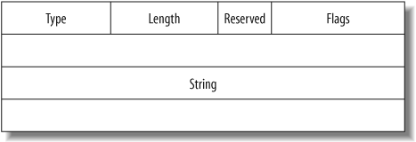
We have a dependency between the string field and the length field. When the layer is assembled, the length field must take its value from the string field. When the layer is dissected, the string field must know the length field value to know where to stop. For the length field, FieldLenField class will be used. It is able to takes its value from the length of another field for assembly. The string field will use the StrLenField class, which is able to use another field's value that is already dissected to know how much bytes to take for the packet at disassembly time.
The type field behavior can be modeled by a ByteField instance. But we can add labels to some type value by using a ByteEnumField instance.
The reserved field is only four bits long. It is modeled by a BitField instance. The number of bits must be passed to its constructor, along with the field's name and default value. BitField instances must be followed by other BitField instances if they do not end on a byte boundary.
The flags field will be modeled by a FlagsField. A FlagsField has almost the same behavior as a BitField except that each bit can be addressed independently. For this, a list of labels is provided, either in the form of a string whose characters are associated with bits or in the form of a list of labels. In this case, we will use the label A for bit 0, B for bit 1, and so on until bit 12.
The length field will be modeled by a FieldLenField instance. The FieldLenField class does not impose any encoding length. By default, it is on two bytes, so we must enforce it to be on one byte with the "B" directive (these directives come from the Python struct module). The field whose length must be measured when the value must be automatically computed is also provided.
The string field will be modeled by a StrLenField instance. It differs from a simple StrField instance by the fact its length is imposed by another field, whose name must be provided.
Example 6-9 shows an initial implementation of the demonstration layer class.
Example 6-9. First implementation of the demonstration layer
class Demo(Packet):
    name = "Demo"
    fields_desc = [ ByteEnumField("type", 2, { "type1":1, "type2":2 }),
                    FieldLenField("length", None, "string", "B"),
                    BitField("reserved", 0, 4),
                    FlagsField("flags", 42, 12, "ABCDEFGHIJKL"),
                    StrLenField("string", "default", "length") ]
Once the class is defined, we can play with it right away:
>>> a=Demo(  )
>>> a.show(  )
###[ Demo ]###
  type= type2
  length= 0
  reserved= 0
  flags= BDF
  string= 'default'
>>> a.flags
42
>>> a.flags=0xF0
>>> a.sprintf("%flags%")
'EFGH'
>>> hexdump(a)
0000   02 07 00 F0 64 65 66 61  75 6C 74                  ....default
>>> a.string="X"*33
>>> hexdump(a)
0000   02 21 00 F0 58 58 58 58  58 58 58 58 58 58 58 58   .!..XXXXXXXXXXXX
0010   58 58 58 58 58 58 58 58  58 58 58 58 58 58 58 58   XXXXXXXXXXXXXXXX
0020   58 58 58 58                                        XXXX
Now you have to inform Scapy of when to use this layer. Let's say it is a protocol that works on UDP packets with source and destination ports of 31337. We will bind it with:
>>> bind_layers(UDP, Demo, sport=31337, dport=31337)
Not only will it make UDP recognize Demo and set ports accordingly:
>>> IP()/UDP()/Demo(  )
<IP  frag=0 proto=udp |<UDP  sport=31337 dport=31337 |<Demo  |>>>
but Scapy will also know it must call the Demo layer when it meets such UDP ports during a dissection:
>>> a=IP()/UDP()/Demo(  )
>>> IP(str(a))
If you need to test new protocols or functions you are developing and you want to use them inside Scapy, you do not need to modify Scapy's source code. Scapy provides a way to launch its own interpreter loop, which takes care of history, completion, etc. You need only to call the scapy.interact( ) function, as Example 6-10 shows.
Example 6-10. Creating a Scapy add-on
#! /usr/bin/env python
# Set log level to benefit from Scapy warnings
import logging
logging.getLogger("scapy").setLevel(1)
from scapy import *
class Test(Packet):
    name = "Test packet"
    fields_desc = [ ShortField("test1", 1),
                    ShortField("test2", 2) ]
def make_test(x,y):
    return Ether()/IP(  )/Test(test1=x,test2=y)
if __name__ == "__main_  _":
    interact(mydict=globals(  ), mybanner="Test add-on v3.14")
You can also use Scapy as a library to create autonomous tools.
Here are several examples of Scapy add-ons that you could create. Example 6-11 is a machine enumeration tool that uses APR ping. Example 6-12 uses ARP requests to exploit etherleak. Add-ons can vary in complexity, even for the same task: Example 6-13 is a very basic ARP traffic monitor, while Example 6-14 is a much more complex ARP traffic monitor.
Example 6-11. Machine enumeration tool using ARP ping
#! /usr/bin/env python
import sys
if len(sys.argv) != 2:
    print "Usage: arping <net>\n  eg: arping 192.168.1.0/24"
    sys.exit(1)
from scapy import srp,Ether,ARP,conf
conf.verb=0
ans,unans=srp(Ether(dst="ff:ff:ff:ff:ff:ff")/ARP(pdst=sys.argv[1]),
              timeout=2)
for s,r in ans:
    print r.sprintf("%Ether.src% %ARP.psrc%")
Example 6-12. Etherleak exploit with ARP requests
#! /usr/bin/env python
from scapy import *
from select import select
target=sys.argv[1]
try:
    s = conf.L2socket(filter="arp")
    while 1:
        can_recv,can_send,err = select([s],[s],[],0)
        if can_recv:
            p = s.recv(  )
            if Padding in p:
                print linehexdump(p[Padding].load)
        if can_send:
            s.send(Ether(  )/ARP(pdst=target))
except KeyboardInterrupt:
    print "Interrupted by user"
Example 6-13. Simplistic ARP traffic monitor
#! /usr/bin/env python
from scapy import *
def arp_monitor_callback(pkt):
    if ARP in pkt and pkt[ARP].op in (1,2): #who-has or is-at
        return pkt.sprintf("%ARP.hwsrc% %ARP.psrc%")
sniff(prn=arp_monitor_callback, filter="arp", store=0)
Example 6-14. More elaborate ARP traffic monitor
#! /usr/bin/env python
from scapy import *
DB = {}
def scarpwatch_callback(pkt):
    if ARP in pkt:
        ip,mac = pkt[ARP].psrc, pkt[ARP].hwsrc
        if ip in DB:
            if mac != DB[ip]:
                if Ether in pkt:
                    target = pkt[Ether].dst
                else:
                    target = "%s?" % pkt[ARP].pdst
                return "poisoning attack: target=%s victim=%s attacker=%s" % \
                       (target, ip, mac)
        else:
            DB[ip]=mac
            return "learned %s=%s" % (mac,ip)
    elif IP in pkt:
        sip,dip = pkt[IP].src, pkt[IP].dst
        if sip not in DB or dip not in DB:
            return
        if Ether in pkt:
            smac,dmac = pkt[Ether].src, pkt[Ether].dst
        elif Dot11 in pkt:
            p11 = pkt[Dot11]
            if p11.FCfield & 3 == 0: # direct
                smac,dmac = p11.addr2,p11.addr1
            elif p11.FCfield & 3 == 1: # to-DS
                smac,dmac = p11.addr3,p11.addr1
            elif p11.FCfield & 3 == 2: # from-DS
                smac,dmac = p11.addr2, p11.addr3
            else:
                smac, dmac = p11.addr4,p11.addr3
        for ip,mac in [(sip,smac), (dip,dmac)]:
            if ip in DB:
                if DB[ip] != mac:
                    return "%s spoofed by %s" % (ip, mac)
sniff(store=0, prn=scarpwatch_callback)Sometimes, network tests have to be repeated on a regular basis. This can be because of unit testing, regression tests, or just network health checks.
UTscapy is a program that drives Scapy in a way that is useful for running test campaigns. Each test is a list of Scapy commands that would have been typed into the Scapy prompt. Tests are grouped by test sets, and a test campaign is compounded of many test sets. Tests and test sets have a title, and optionally, keywords and comments.
The file format of a test campaign is quite simple. Everything that begins with a # is ignored and can be used for comments. The campaign title is introduced by %, test set titles by +, unit test titles by =, comments by *, and keywords by ˜. Example 6-15 shows all of the elements of a test campaign file.