5
Microeconomic Models
This chapter contains four microeconomic models that illustrate important themes in political economy. Readers who want to be able to analyze economic problems themselves from a political economy perspective are encouraged to work through these models.
Model 5.1: The Public Good Game
The “public good game” illustrates why markets will allocate too few of our scarce productive resources to the production of public, as opposed to private goods. Assume 0, 1, or 2 units of a public good can be produced and the cost to society of producing each unit is $11. Either Ilana or Sara can purchase 1 unit, or none of the public good – each paying $11 if she purchases a unit, and nothing if she does not. Suppose Sara gets $10 of benefit for every unit of the public good that is available and Ilana gets $8 of benefit for every unit available. We fill in a game theory “payoff matrix” for each woman buying, or not buying, one unit of the public good as follows: We calculate the net benefit for each woman by subtracting what she must pay if she purchases a unit of the public good from the benefits she receives from the total number of the public good produced and therefore available for her to consume. Ilana’s payoff is listed first, and Sara’s second in each “cell.” For example, in the case where both Ilana and Sara buy a unit of the public good, and therefore each gets to consume 2 units of the public good, Ilana’s net benefit is 2($8) – $11, or $5, and Sara’s net benefit is 2($10) – $11, or $9.
(1) Will Sara buy a unit? No. Sara is better off free riding no matter what Ilana does. If Ilana buys, Sara is better off not buying and free riding since $10 > $9. If Ilana does not buy Sara is also better off not buying than buying since $0 > – $1.
| SARA | |||
| Buy | Free Ride | ||
| ILANA | Buy | ($5, $9) | (–$3, $10) |
| Free Ride | ($8, –$1) | ($0, $0) | |
(2) Will Ilana buy a unit? No. Ilana is also better off free riding no matter what Sara does since $8 > $5 and $0 > – $3.
(3) Assuming that Sara and Ilana’s benefits are of equal importance to society, what is the socially optimal number of units of the public good to produce? 2 units since $5 + $9 = $13 is greater than $10 – $3 = $8 – $1 = $7 which is greater than $0 + $0 = $0.
Suppose the social cost and price a buyer is charged is $5 instead of $11. The game theory payoff matrix for buying or not buying one unit of the public good now is:
| SARA | |||
| Buy | Free Ride | ||
| ILANA | Buy | ($11, $15) | ($3, $10) |
| Free Ride | ($8, –$5) | ($0, $0) | |
(4) Will Sara buy a unit? Yes. Buying is best for Sara no matter what Ilana does since $15 > $10 if Ilana buys, and $5 > $0 if Ilana does not buy.
(5) Will Ilana buy a unit? Yes. Buying is best for Ilana no matter what Sara does since $11 > $8 if Sara buys, and $3 > $0 if Sara does not buy.
(6) Assuming that Sara and Ilana’s benefits are of equal importance to society, what is the socially optimal number of units of the public good to produce? 2 units yields the largest possible net social benefit of any of the four possible outcomes: $11 + $15 = $26.
Finally, suppose the social cost and price a buyer is charged is $9. Now the game theory payoff matrix for buying or not buying one unit of the public good is:
| SARA | |||
| Buy | Free Ride | ||
| ILANA | Buy | ($7, $11) | (–$1, $10) |
| Free Ride | ($8, $1) | ($0, $0) | |
(7) Will Sara buy a unit? Yes, since Sara is better off buying no matter what Ilana does: $11 > $10 when Ilana buys, and $1 > $0 when Ilana does not buy.
(8) Will Ilana buy a unit? No, since Ilana is better off free riding no matter what Sara does: $8 > $7 when Sara buys, and $0 > –$1 when Sara does not buy.
(9) Assuming that Sara and Ilana’s benefits are of equal importance to society, what is the socially optimal number of units of the public good to produce? 2 units since $7 + $11 = $18 is greater than $8 + $1 = $10 – $1 = $9, which is greater than $0 + $0 = $0.
What the “public good game” demonstrates is the following conclusion: Unless the private benefit to each consumer of a unit of a public good exceeds the entire social cost of producing a unit, the free rider problem will lead to underproduction of the public good. When the cost is $11 the private benefit for both Sara and Ilana is less than the social cost, and neither buys, although buying and consuming two units is socially beneficial. When the cost is $9 the private benefit for Ilana is still less than the social cost so she does not buy, and only one unit is bought (by Sara) and consumed (by both women), although producing and consuming two would be more efficient. Only when the cost is $5 is the private benefit to both Sara and Ilana sufficient to induce each to buy, and then and only then do we get the socially efficient level of public good production. Obviously for most public goods the private benefit to most individual buyers will not outweigh the entire social cost of producing the public good, and we will therefore get significant “underproduction” of public goods if resource allocation is left to the free market.
Model 5.2: The Price of Power Game
When people in an economic relationship have unequal power the logic of preserving a power advantage can lead to a loss of economic efficiency. This dynamic is illustrated by the “Price of Power Game” which helps explain phenomena as diverse as why employers sometimes choose a less efficient technology over a more efficient one, and why patriarchal husbands sometimes bar their wives from working outside the home even when household wellbeing would be increased if the wife did work outside.
Assume P and W combine to produce an economic value and divide the benefit between them. They have been producing a value of 15, but because P has a power advantage in the relationship P has been getting twice as much as W. So initially P and W jointly produce 15, P gets 10 and W gets 5. A new possibility arises that would allow them to produce a greater value. Assume it increases the value of what they jointly produce by 20%, i.e. by (0.20)(15) = 3, raising the value of their combined production from 15 to 15 + 3 = 18. But taking advantage of the new, more productive possibility also has the effect of increasing W’s power relative to P. Assume the effect of producing the greater value renders W as powerful as P eliminating P’s power advantage in their relationship. The obvious intuition is that if P stands to lose more from receiving a smaller slice than P stands to gain from having a larger pie to divide with W, it will be in P’s interest to block the efficiency gain. We can call this efficiency loss “the price of power.” But constructing a simple “game tree” helps us understand the obstacles that prevent untying this Gordian knot as well as the logic leading to the unfortunate result.
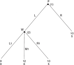
Figure 5.1 Price of Power Game
As the player with the power advantage P gets to make the first move at the first “node.” P has two choices at node 1: P can reject the new, more productive possibility and end the game. We call this choice R (for “right” in the game tree diagram in Figure 5.1), and the payoff for P is 10 (listed on top) and the payoff for W is 5 (listed on the bottom) if P chooses R. Or, P can defer to W allowing W to choose whether or not they will adopt the new possibility. We call this choice L (for “left” in the game tree diagram in Figure 5.1), and the payoffs for P and W in this case depend on what W chooses at the second node. If the game gets to the second node because P deferred to W at the first node, W has three choices at node 2: Choice R1 is for W to reject the new possibility in which case the payoffs remain 10 for P and 5 for W as before. Choice L1 is for W to choose the new, more productive possibility and insist on dividing the larger value of 18 equally between them since the new process empowers W to the extent that P no longer has a power advantage, and therefore W can command an equal share with P. If W chooses L1 the payoff for P is therefore 9 and the payoff for W is also 9. Finally, choice M1 (for “middle” in the game tree in Figure 5.1) is for W to choose the new, more productive possibility but to offer to continue to split the pie as before, with P receiving twice as much as W. In other words, in M1 W promises P not to take advantage of her new power, which means that P still gets twice as much as W, but since the pie is larger now P’s payoff is 12 and W’s payoff is 6 if W chooses M1 at node 2.
We solve this simple dynamic game by backwards induction. If given the opportunity, W should choose L1 at node 2 since W receives 9 for choice L1 and only 5 for choice R1 and only 6 for choice M1. Knowing that W will choose L1 if the game goes to node 2, P compares a payoff of 10 by choosing R with an expected payoff of 9 if P chooses L and W subsequently chooses L1 as P has every reason to believe she will. Consequently P chooses R at node 1 ending the game and effectively “blocking” the new, more productive possibility.
The outcome of the game is not only unequal – P continues to receive twice as much as W – it is also inefficient. One way to see the inefficiency is that while P and W could have produced and shared a total value of 18 they end up only producing and sharing a total value of 15. Another way to see the inefficiency is to note that there is a Pareto superior outcome to (R). (L, M1) is technically possible and has a payoff of 12 for P and 6 for W, compared to the payoff of 10 for P and 5 for W that is the “equilibrium outcome” of the game.
It is the existence of L1 as an option for W at node 2 that forces P to choose R at node 1. Notice that if L1 were eliminated so that W had only two choices at node 2, R1 and M1, W would choose M1 in this new game, in which case P would choose L instead of R at node 1. While this outcome would remain unequal it would not be inefficient. So one could say the inefficiency of the outcome to the original game is because W cannot make a credible promise to P to reject option L1 if the game gets to node 2. Since there is no reason for P to believe W would actually choose M1 over L1 if the game gets to node 2, P chooses R at node 1. In effect P will block an efficiency gain whenever it diminishes P’s power advantage sufficiently. If P stands to lose more from a loss of power than he gains from a bigger pie to divide, P will use his power advantage to block an efficiency gain.1
If we turn our attention to how the efficiency loss might be avoided, two possibilities arise. The most straightforward solution, which not only avoids the efficiency loss but generates equal instead of unequal outcomes for P and W, is to eliminate P’s power advantage. If P and W have equal power and divide the value of their joint production equally they will always choose to produce the larger pie and there will never be any efficiency losses. The more convoluted solution is to accept P’s power advantage as a given, and search for ways to make a promise from W not to take advantage of her enhanced power credible. Is there some way to transform the initial game so that a promise from P not to choose L1 is credible?
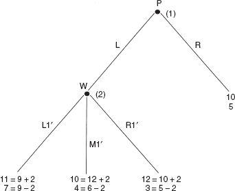
Figure 5.2 Transformed Price of Power Game
What if W offered P 2 units to choose L rather than R at node 1? If a contract could be devised in which W had to pay P 2 units, if and only if P chose L at node 1, then the new game would have the following payoffs at node 2: If W chose R1' P would get 10 + 2 = 12 instead of 10, and W would get 5 – 2 = 3 instead of 5. If W chose M1' P would get 12 + 2 = 14 instead of 12 and W would get 6 – 2 = 4 instead of 6. Finally, if W chose L1' P would get 9 + 2 = 11 and W would get 9 – 2 = 7 instead of 9. Under these circumstances, in the transformed price of power game illustrated in Figure 5.2 W would choose L1' since 7 is greater than both 4 and 3. But when W chooses L1' at node 2 that gives P 11 which is more than P gets by choosing R at node 1. Therefore a bribe of 2 paid by W to P if and only if P chooses R over L would give us an efficient but unequal outcome. It is efficient because P and W produce 18 instead of 15 and because (L, L1') is Pareto superior to (R). It is still unequal because P receives 11 while W receives only 7.
There are many economic situations where implementing an efficiency gain changes the bargaining power between collaborators and therefore the Price of Power Game can help illustrate aspects of what transpires. Below are two interesting applications.
If P is a patriarchal head of household and W is his wife, the game illustrates one reason why the husband might refuse to permit his wife to work outside the home even though net benefits for the household would be greater if she did.2 Patriarchal power within the household can be modeled as giving the husband the “first mover advantage” in our model. Patriarchal power in the economy can be modeled as a gender wage gap for women with no labor market experience. If we assume as long as the wife has not worked outside the home she cannot command as high a wage as her husband in the labor market, her exit option is worse than her husband’s should the marriage dissolve. This unequal exit option makes it possible for a patriarchal husband to insist on a greater share of the household benefits than the wife as long as she has no outside work experience.3 But after she works outside the home for some time the unequal exit option can dissipate, and with it the husband’s power advantage within the home.
The obstacles to eliminating efficiency losses in this situation by eliminating patriarchal advantages are not economic. Gender-based wage discrimination can be eliminated through effective enforcement of laws outlawing discrimination in employment such as those in the US Civil Rights Act. The psychological dynamics that give “first mover” advantages to husbands within marriages require changes in the attitudes and values of both men and women about gender relations. Of course eliminating the efficiency loss due to patriarchal power by eliminating patriarchal power has the supreme advantage of improving economic justice as well as efficiency.
Trying to eliminate the efficiency loss by making the wife’s promise not to exercise the power advantage she gets by working outside the home credible has a number of disadvantages. Most importantly it is grossly unfair. The bribe the wife must pay her husband to be “allowed” to work outside the home is obviously the result of the disadvantages she suffers from having to negotiate under conditions of unequal and inequitable bargaining power in the first place. Second, it may not be as “practical” as it first appears. Those who believe this solution is more “achievable” than reducing patriarchal privilege should bear in mind how unlikely it is that wives with no labor market credentials could obtain what would amount to an unsecured loan against their future expected productivity gain! Nor could their husbands co-sign for the loan without effectively changing the payoff numbers in our revised game. Third, even if wives obtained loans from some outside agent – presumably an institution like the Grameen Bank in Bangladesh that gives loans to women without collateral but holds an entire group of women responsible for non-payment of any individual – there would have to be a binding legal contract that prevented husbands from taking the bribe and reneging on their promise to allow their wives to work outside the home. Notice that if P can take the bribe and still choose R he gets 10 + 2 = 12 which is greater than the 11 he gets if he keeps his promise to choose L.
Finally, notice that any bribe between 1 and 4 would successfully transform the game from an inefficient power game to a conceivably efficient, but nonetheless inequitable power game. If W paid P a bribe of 4 the entire efficiency gain would go to her husband. But even if W paid P only a bribe of 1 and kept the entire efficiency gain for herself, she would still end up with less than her husband. In that case W would get 9 – 1 = 8 compared to 9 + 1 = 10 for P. So even if we conjure up a Grameen Bank to give never employed women unsecured loans, even if we ignore all problems and costs of enforcement, there is no way to transform our power game into a game that would deliver efficient and equitable outcomes. Since P gets 10 by choosing R and ending the game, he must receive at least 10 in order to choose L. But if the productivity gain is only 3 when both work outside, and therefore total household net benefits are only 18, W can receive no more than 8 if P must have at least 10, and no transformation of the game that preserves patriarchal power will produce equitable results. Whether or not this morally inferior solution is actually easier to achieve than reducing patriarchal privilege also seems to be an open question.
If P represents an employer, or “Patron,” and W represents his employees or “Workers,” the Price of Power Game illustrates why an employer might fail to implement a new, more productive technology if that technology is also “worker empowering.” A host of factors influence the bargaining power between employers and employees, and therefore the wages employees will receive and the efforts they will have to exert to receive them. But one factor that can affect bargaining power in the capitalist firm is the technology used. For example, if an assembly line technology is used and employees are physically separated from one another and unable to communicate during work, it may be more difficult for employees to develop solidarity that would empower them in negotiations with their employer as compared to a technology that requires workers to work in teams with constant communication between them. Or it may be that one technology requires employees themselves to have a great deal of know-how to carry out their tasks, while another technology concentrates crucial productive knowledge in the hands of a few engineers or supervisors, rendering most employees easily replaceable and therefore less powerful. If the technology that is more productive is also “worker empowering,” employers face the dilemma illustrated by our Price of Power Game and may have reason to choose a less efficient technology over a more efficient one that is more worker empowering.
When we consider possible solutions in this application an interesting new wrinkle arises. In capitalism there is inevitably a conflict between employers and employees over wages and effort levels. If new technologies not only affect economic efficiency but the relative bargaining power of employers and employees as well, we cannot “trust” the choice of technology to either interested party without running the risk that a more productive technology might be blocked due to detrimental bargaining power effects for whoever has the power to choose. I pointed out above how P might block a more efficient technology if it were sufficiently employee empowering, so we cannot trust employers to choose between technologies. But if W had the power to do so, W might block a more efficient technology if it were sufficiently employer empowering, so it appears we cannot resolve the dilemma by giving unions the say over technology in capitalism either. Since we cannot change the fact that new more productive technologies sometimes affect bargaining power, the solution seems to lie in eliminating the conflict between employers and employees. This can only happen in economies where there are no employers and no division between profits and wages, that is, in economies where employees manage and pay themselves. We consider economies of this kind in Chapter 11.
Model 5.3: Climate Control Treaties
This exercise is designed to illustrate some of the key issues when designing an international climate treaty that is effective – reduces global emissions sufficiently – equitable – distributes responsibility for reductions according to differential responsibility and capability – and efficient – minimizes the global cost of averting climate change. Imagine three countries sitting down to negotiate a climate treaty: the United States, Russia, and India. Consider the United States and Russia as more developed countries (MDCs), termed Annex-1 countries in the Kyoto Protocol, and India as a less developed country (LDC), or a non-Annex-1 country. Below are equations for both the marginal costs (MCs) and total costs (TCs) of reducing greenhouse gas (GHG) emissions for all three countries. As a country reduces emissions more and more, the MC of reducing emissions rises. This is because presumably a country will use the least costly options for reducing emissions first, and move on to higher-cost methods as more emission reductions are required. It is also typically the case that the MC of emission reduction is lower in developing countries. This is because LDCs have engaged in relatively little emission reduction, or abatement, so many low-cost opportunities for reducing emissions are still available in LDCs. The MC and TC of emissions reduction (abatement) for the three countries are expressed in billions of dollars, where X is the number of tons of GHG emissions reduced:
| United States | MCus = 5XUS | TCus = 2.5XUS2 |
| Russia | MCR = 2XR | TCR = XR2 |
| India | MCI = XI | TCI = XI2/2 |
No Treaty
Initially there is no treaty. And while each country has potentially unlimited “rights” to emit carbon into the upper atmosphere, the United States chooses only to “exercise” its “right” to emit 400 tons, Russia chooses only to exercise its right to emit 250 tons, and India chooses only to exercise its right to emit 200 tons. As a result, global emissions are 850 tons. Suppose the international community has identified a 10% reduction in global carbon emissions as necessary to reduce the risk of dangerous climate change to an acceptable level.
Treaty 1 requires each country to reduce its emissions by 10%
(1) |
How much emission reduction would each country have to do? |
|
United States: |
(0.10)400 = 40 = XUS |
|
| Russia: | (0.10)250 = 25 = XR | |
| India: | (0.10)200 = 20 = XI | |
| Global: | (40 + 25 + 20) = 85 = XG = (0.10)850 | |
(2) |
What would be the cost of the last ton of emission reduced in each country? |
|
United States: |
MCUS = 5XUS = 5(40) = $200 |
|
| Russia: | MCR =2XR = 2(25) = $50 | |
| India: | MCI = XI = 1(20) = $20 | |
(3) |
What would be the total cost for each country? |
|
United States: |
TCUS = 2.5XUS2 = 2.5(40)2 = $4,000 |
|
| Russia: | TCR = XR2 = (25)2 = $625 | |
| India: | TCI = XI2/2 = (20)2 /2 = $200 | |
(4) |
What would be the total cost of emission reduction for the world? |
|
TCG = $4,000 + $625 + $200 = $4,825 |
||
Efficiency After each country has reduced its emissions by 10%, the MC of reduction is different in the three countries. We therefore know we failed to minimize the global cost of reduction, which means the pattern of reductions this treaty yields is inefficient. To illustrate: The last ton reduced in the United States (the 40th ton reduced) cost $200, while the last ton reduced in Russia (the 25th ton reduced) cost only $25. Had we reduced 39 tons in the United States (instead of 40) and 26 tons in Russia (instead of 25), we would have achieved the same level of global reductions, 85, but global cost would have been $200 – $25 = $175 lower.
Equity For simplicity assume the benefits of achieving a global reduction of 85 tons are the same for all three countries. While the United States is paying more than Russia, which is paying more than India to achieve this global reduction, we might argue that it is still unfair for India to bear this much of the cost because (1) India did much less to create the problem in the first place since Indian per capita cumulative emissions are much lower than per capita cumulative emissions of the United States and Russia, and (2) India is less able to bear the cost of preventing climate change since per capita gross domestic product (GDP) is much lower there. We could also argue that the treaty now explicitly limits each country’s “right” to release carbon into the upper atmosphere but distributes the remaining rights very unfairly. The treaty implicitly awards the United States rights to emit (400 – 40) = 360 tons, but awards Russia only rights to emit (250 – 25) = 225 tons, and India only rights to emit (200 – 20) = 180 tons. Other ways to see why this treaty is unfair are: (1) Since per capita cumulative emissions are highest in the United States and lowest in India, India should be awarded the most rights to emit more carbon dioxide in the future and the United States should be awarded the fewest rights to emit more – whereas this treaty does just the opposite. (2) Since emission rights are a new form of wealth and per capita wealth is lowest in India and highest in the United States, India should receive the most emission rights and the United States the fewest – whereas this treaty does just the opposite. (3) It is more difficult to achieve economic development when consumption of fossil fuel is limited. Since India is least developed and the United States is most developed, India should receive the most emission rights and the United States the fewest – whereas this treaty does just the opposite.
Treaty 2 calls for a 10% reduction in global emissions, but exempts India from making any reductions and permits no trading of emission rights
Efficiency Treaty 2 is even less efficient than Treaty 1 since $7,909.09 > $4,825. This is why people sometimes argue that achieving equity can come at the expense of efficiency. The cost of treating India fairly – not requiring it to reduce emissions at all – has raised the global cost of reducing emissions by 85 tons by $7,909.09 – $4,825 = $3,084.09. The reason is that none of the reduction is taking place in India, where the costs of reduction are lowest. Note that the first unit reduced in India would have cost only $1! We are also distributing reductions inefficiently between the United States and Russia since the MCs are different in these two countries. We could lower TCG by having more of the reductions in Russia, where the last unit of abatement cost only $65.38, and fewer of the reductions in the United States, where the last unit of abatement cost $261.54. But since Treaty 2 does not permit carbon trading between the United States and Russia, the inefficient pattern of abatement in those two countries will not be eliminated.
Equity Clearly Treaty 2 treats India more fairly than Treaty 1 does. The implicit distribution of emissions rights – that is, new wealth – is now, for the United States, 400 – 52.308 = 347.692 (which is less than 360), and for Russia, 250 – 32.692 = 217.308 (which is less than 225). While India is given potentially limitless emission rights, under Treaty 2 India will only “exercise” its rights to emit 200 tons. That is all India chose to exercise before there was any treaty, and since this treaty does not allow India to sell any of its new wealth, India will continue to emit 200 tons, as before.
Treaty 3 calls for a 10% reduction in global emissions, exempts India from making any reductions, reduces US and Russian emission rights by the same percentage – 13.077 – but permits unlimited trading of emission rights between Annex-1 countries (that is, between the United States and Russia)
(1) |
How much would each country have to reduce its emissions? Once again XUS + XR = 85 and XI = 0. But now instead of 400 p + 250 p = 85, meaning that the United States and Russia will each reduce its emissions by the same percentage, p, the pattern of emissions reductions will be determined by the condition: MCUS = MCR. This is because the United States and Russia will keep trading emission rights until there are no longer any mutually beneficial deals to be struck, which will be the case only when MCUS becomes equal to MCR. So 5XUS = MCUS = MCR = 2XR, or XUS = (2/5)XR. Substituting for XUS in the first equation above, (2/5)XR + XR = 85, and XR = (5/7)85 = 60.714, and therefore XUS = 24.286. |
|
United States: |
24.286 = XUS |
|
| Russia: | 60.714 = XR | |
| India: | 0 = XI | |
| Global: | 24.286 + 60.286 + 0 = 85 = XG | |
(2) |
What would be the cost of the last ton of emission reduced in each country? |
|
United States: |
MCUS = 5XUS = 5(24.286) = $121.43 |
|
| Russia: | MCR = 2XR = 2(60.714) = $121.43 | |
| India: | [Note: MCI = XI = 1(1) = $1 if India reduced emissions by 1 ton] | |
(3) |
What would be the total cost of the reductions carried out in each country? |
|
United States: |
TCUS = 2.5XUS2 = 2.5(24.286)2 = $1,474.52 |
|
| Russia: | TCR = XR2 = (60.714)2 = $3,686.19 | |
| India: | TCI = XI2/2 = (0)2 /2 = $ 0.00 | |
However, the total cost to the United States is not just the cost of reducing its own emissions by 24.286 tons. That reduction is not sufficient to achieve a 13.077% reduction from 400, i.e. to get down to 347.692 tons, which is all the United States has the “right” to emit. Consequently, the United States will have to buy emission rights from Russia to meet its treaty obligations: 400 – 24.286 = 375.714 tons emitted – 347.692 tons allowed = 28.022 emission permits the US must buy from Russia. The price of each emission right will be $121.43 because Russia would accept no less (since that is what it will cost Russia to reduce its last ton), and the United States will pay no more (since the United States could reduce another ton itself for that amount). So $121.43(28.022) = $3,402.71, and the total cost to the United States – that is, the cost of reducing emissions internally by 24.286 tons, plus the cost of buying 28.022 emission rights from Russia – is $1,474.52 + $3,402.71 = $4,877.23. |
||
The total cost to Russia of reducing emissions by 60.714 – which exceeds a 13.077% reduction from 250 by 28.022 tons – is reduced by the amount Russia gains from selling 28.022 emission rights to the United States. At a price of $121.43 each, Russia reduces its total costs by $121.43(28.022) = $3,402.71. So the total cost to Russia – that is, the cost of reducing emissions internally by 60.714 tons, minus the revenue received from selling 28.022 emission rights to the United States – is $3,686.19 – $3,402.71 = $283.48. | ||
(4) What would be the total cost of emissions reduction for the world?
TCG = $4,877.23 + $283.48 + $0 = $5,160.71
(Alternatively: TCG = $1,474.52 + $3,686.19 + $0 = $5,160.71)
Efficiency Treaty 3 is more efficient than Treaty 2 because it allows reductions to be reallocated from the United States to Russia until the marginal reduction costs are equal in the two countries. TCG are lowered by $7,909.09 – $5,160.71 = $2,748.38. However, Treaty 3 is still not as efficient as it might be. The 85th ton reduced costs $121.43 (whether it is reduced in the United States or in Russia). If instead the 85th ton were reduced in India, it would cost only $1!
Equity The distribution of emission rights under Treaty 3 is the same as under Treaty 2, so the equity implications of the wealth distribution are the same. The efficiency gain ($7,909.09 – $5,160.71 = $2,748.38) from reallocating reductions from the United States to Russia until the marginal reduction costs are equal in the two countries achieved by Treaty 3 is divided between the United States ($6,840.32 – $4,877.23 = $1,963.09) and Russia ($1,068.77 – $283.48 = $785.29). There is no change for India. Under both Treaty 2 and Treaty 3, India benefits from prevention of climate change at no cost.
Treaty 4 calls for a 10% reduction in global emissions, continues to exempt India from responsibility for any reductions, reduces US and Russian emission rights by the same percentage – 13.077 – but permits unlimited trading of emissions rights between all countries, including India; that is, full use of a Clean Development Mechanism (CDM). This treaty most closely resembles the treaty negotiated in Kyoto in 1997 which was in effect from 2005 through 2012
However, the United States and Russia will have to buy emission rights from India as follows: |
||
The United States will buy: |
400 – (1 – 0.13007)400 – 10 = 42.308 |
|
| Russia will buy: | 250 – (1 – 0.13007)250 – 25 = 7.692 | |
| India will sell: | 42.308 + 7.692 = 50 | |
Emission rights will sell for $50 each because the MC of reductions is now $50 in all three countries, so no country will pay more than $50 for a credit or sell a credit for less than $50. Therefore, it will cost the United States an additional $50(42.308) = $2,115.40, it will cost Russia an additional $50(7.692) = $384.60, and India will gain $50(50) = $2,500 from selling emission rights through the CDM, and therefore the total costs for the three countries are: |
||
United States: |
TCUS = $250 + $2,115.40 = $2,365.40 |
|
| Russia: | TCR = $625 + $384.60 = $1,009.60 | |
| India: | TCI = $1,250 – $2,500.00 = – $1,250.00 | |
(4) |
What would be the total cost of emission reductions for the world? TCG = $2,365.40 + $1,009.60 – $1,250 = $2,125 (also TCG = $250 + $625 + $1,250 = $2,125) |
|
Efficiency: Treaty 4 has minimized the global cost of reducing global emissions by 85 tons: TCG for Treaty 4 = $2,125 < TCG for Treaty 1 = $4,825 < TCG for Treaty 3 = $5,160.71 < TCG for Treaty 2 = $7,909.09. We also know this because the marginal costs of reduction are the same in all three countries, so there is no way to reallocate emission reductions and lower global costs. Comparing the total cost of reducing emissions by 85 tons under Treaty 4 and Treaty 3, the efficiency gain produced by the CDM is $5,160.71 – $2,125 = $3,035.71. It is distributed as follows: US total costs have fallen by $4,877.23 – $2,365.40 = $2,511.83. Russian total costs have risen by $1,009.60 – $283.48 = $726.12. (This is because the CDM allowed India to replace Russia as the seller in the lucrative market for emission rights.) And India now enjoys a profit of $1,250.
Equity Treaty 4 awards the same emission rights – that is, new wealth – as Treaty 2 and 3: the United States (347.692), Russia (217.308), and India (potentially limitless). However, the CDM in Treaty 4 allows India to make more profitable use of its emission rights by selling some of them to the United States and Russia. Under Treaty 2 and 3, India could not sell any of its new wealth to the United States and Russia. The CDM allows India to sell emission rights, which it has every incentive to do as long as reducing emissions costs less than the price India receives. In the market for emission rights, supply (50 emission rights supplied by India) will equal demand for emission rights (42.308 from the United States plus 7.692 from Russia) when the price of an emission right is $50. So under Treaty 4 the reduction of 50 of the 85 tons reduced globally will take place in India, which will presumably (see below) cut back on its emissions from 200 to 150 tons. However, even though the reductions are taking place in India (where they are cheaper), the costs of achieving those reductions are being paid for by the United States and Russia.
The United States and Russia are paying more than it costs India to reduce 50 tons. The total cost of reducing the 50 tons in India is 502/2 = $1,250. The United States and Russia pay India $50(50) = $2,500. But this does not mean the United States and Russia are overpaying India by $1,250. We could just as easily argue the United States and Russia are underpaying India because it would have cost the United States and Russia much more than $2,500 to reduce those 50 tons themselves. By comparing the total costs under Treaty 3 and Treaty 4, we can calculate how much more it would have cost the United States and Russia: From Treaty 3 we know the total cost to the United States and Russia combined of reducing all 85 tons themselves is $5,160.71. From Treaty 4 the total cost to the United States and Russia combined (when they can purchase 50 of the 85 tons from India) is $2,365.40 + $1,009.60 = $3,375. Therefore the United States and Russia have saved $5,160.71 – $3,375 = $1,785.71 by purchasing 50 emission rights from India. Rather than speak of over or underpaying, it is more accurate to say that the United States and Russia are sharing with India the efficiency gain from relocating 50 tons of reduction from the United States and Russia to India. In this case, the United States and Russia are getting $1,785.71 of the efficiency gain, and India is getting $1,250 of the efficiency gain.
Warning There is an important implicit assumption in the above analysis and an explicit warning is in order. We have assumed that India will actually reduce its emissions by 50 tons when it sells 50 emission rights to the United States and Russia, and therefore India will only emit 200 – 50 = 150 tons. Of course this is what the executive board of the CDM in the Kyoto Protocol is supposed to ensure when it certifies emission rights for sale, namely that there was actually that number of tons reduced additional to what would have occurred in any case, which was 200. But Treaty 4 gives India unlimited emission rights. When India could not sell emission rights, it only found it in its interest to “exercise” its right to emit 200 tons. But since India can now sell emission rights at $50 apiece, why would India not want to “exercise” its right to emit more than 200 tons – in which case global emissions would no longer decline by 85 tons? As long as India has unlimited emission rights, there will be what economists call a perverse incentive for India to try to sell bogus emission rights. Selling a real reduction that cost only $15, say, for $50 is a good deal. But if you can sell a “pretend” reduction that cost nothing for $50, that is an even better deal!
The simple way to solve this problem is not to give India unlimited emission rights. Requiring India to reduce its emissions by 0.0% means requiring India to maintain its emissions at 200 tons. So all we have to do is give India the right to emit 200 tons – all it wanted to emit initially. Then if India decides it wants to sell 50 of those 200 emission rights to the US and Russia – which it clearly has an incentive to do – it must cut its own emissions back to 150 tons.
This is only an exercise for illustrative purposes. However, readers can find out for themselves what truly fair reductions are for every country in the world by going to the EcoEquity website www.ecoequity.org, and using their “equity calculator.” Readers can chose among three global reduction scenarios, three different weights for responsibility and capability, three different development thresholds, and three different dates from which to calculate historic responsibility. For any combination of choices the calculator will tell you how much each country has a right to continue to emit, and how much each country is responsible for reducing. What the above exercise demonstrates is that when there are significant differences in marginal reduction costs in different countries, if the treaty you design using the EcoEquity calculator – that is the treaty you believe is both effective and fair – permits country governments to authorize the sale and purchase of emission rights by sources: (1) there will be a great deal of trading, (2) which will significantly reduce global reduction costs, and (3) generate a significant flow of payments from sources in MDCs to sources in LDCs.
Model 5.4: The Sraffa Model of Income Distribution and Prices
Mainstream economic theory explains the prices of goods and services in terms of consumer preferences, production technologies, and the relative scarcities of different productive resources. Political economists, on the other hand, have long insisted that wages, profits, and rents are determined by power relations among classes in addition to factors mainstream economic theory takes into account, and therefore that the relative prices of goods in capitalist economies depend also on power relations between classes as well as on consumer preferences, technologies, and resource scarcities.
The labor theory of value Karl Marx developed in Das Kapital was the first political economy explanation of “wage, price and profit”4 determination. In Production of Commodities by Means of Commodities (Cambridge University Press, 1960) Piero Sraffa presented an alternative political economy framework that avoided logical inconsistencies and anomalies in the labor theory of value, and extends easily to include different wage rates for different kinds of labor and rents on different kinds of natural resources – which the labor theory of value cannot accommodate. The model below is based on Sraffa, and is often called “the modern surplus approach.”
The “surplus approach” is only one part of a political economy explanation of the determination of wages, profits, rents, and prices. The surplus approach does not explain why consumers come to have the preferences they do, nor what determines the relative power of employers, workers, and resource owners. Instead the surplus approach takes consumer demand and the power relationships between workers, employers, and resource owners as givens, and seeks to explain what prices will result under those conditions. While it does not explain what causes changes in the power relations between workers, employers, and resource owners, the surplus approach does explain how any changes in power between them will affect prices as well as income distribution. And while it does not explain what causes technological innovations, it does explain which new technologies will be chosen, and how their implementation will affect wages, profits, rents, prices, and economic efficiency. Logically, the surplus approach is the last part of a micro political economy. Other political economy theories must explain the factors that influence preference formation and power relations between different classes. In Chapters 2, 4 and 10 the effects of institutional biases on preference formation are explained briefly. In Chapter 10 factors affecting the bargaining power of workers and capitalists are explored. But once consumer demand and the bargaining power between classes is given, the “surplus approach” provides a rigorous explanation of price formation and income distribution in capitalism.5
Assume a two sector economy defined by the technology below where a(ij) is the number of units of good i needed to produce one unit of good j, and L(j) is the number of hours of labor needed to produce one unit of good j. Suppose:
a(11) = 0.3 a(12) = 0.2
a(21) = 0.2 a(22) = 0.4
L(1) = 0.1 L(2) = 0.2
The first column can be read as a “recipe” for making one unit of good 1: It takes 0.3 units of good 1 itself, 0.2 units of good 2, and 0.1 hour of labor to “stir” these inputs to get 1 unit of good 1 as output. Similarly, the second column is a recipe for making one unit of good 2: It takes 0.2 units of good 1, 0.4 units of good 2 itself, and 0.2 hours of labor to make one unit of good 2.
Let p(i) be the price of a unit of good i, w be the hourly wage rate in the economy, and r(i) be the rate of profit received by capitalists in sector i. The first step is to write down an equation for each industry that expresses the truism that revenue minus cost for the industry is, by definition, equal to industry profit. If we divide both sides of this equation by the number of units of output the industry produces we get the truism that revenue per unit of output minus cost per unit of output must equal profit per unit of output. Another way of saying this is: cost per unit of output plus profit per unit of output must equal revenue per unit of output. This is the equation we want to write for each industry.
The second step is to write down what cost per unit of output and revenue per unit of output will be for each industry. For industry 1 it takes a(11) units of good 1 itself to make a unit of output of good 1. That will cost p(1)a(11). It also takes a(21) units of good 2 to make a unit of output of good 1. That will cost p(2)a(21). So [p(1)a(11) + p(2)a(21)] are the non-labor costs of making one unit of good 1. Since it takes L(1) hours of labor to make a unit of good 1 and the wage per hour is w, the labor cost of making a unit of good 1 is wL(1). Revenue per unit of output of good 1 is simply p(1).
What is profit per unit of output in industry 1? By definition profits are revenues minus costs, so profits per unit of output must be equal to revenues per unit of output minus cost per unit of output. Also by definition the rate of profit is profits divided by whatever part of costs a capitalist must pay for in advance. Dividing both the numerator, profits, and denominator, costs advanced, by the number of units of output in industry 1 gives us the truism that the rate of profit in industry 1 is equal to the profit per unit of output in industry 1 divided by whatever part of costs per unit of output capitalists must advance in industry 1. Therefore, (multiplying both sides of this identity by costs advanced per unit of output) the profit per unit of output in industry 1 must be equal to the rate of profit for industry 1 times the cost per unit of output capitalists must advance in industry 1.
We will assume (with Sraffa) that capitalists must pay for non-labor costs in advance but can pay their employees after the production period is over out of revenues from the sale of the goods produced. So the cost per unit of output capitalists must advance in industry one is only the non-labor costs per unit, or [p(1)a(11) + p(2)a(21)]. We will also assume (with Sraffa) that the rate of profit capitalists receive is the same in both industries, r.6 Therefore:
profit per unit of output in industry one = r[p(1)a(11) + p(2)a(21)]
And we are ready to write the accounting identity, or truism, that cost per unit of output plus profit per unit of output equals revenue per unit of output in industry 1:
[p(1)a(11) + p(2)a(21)] + wL(1) + r[p(1)a(11) + p(2)a(21)] = p(1)
Which can be rewritten for convenience as:
(1) (1+r) [p(1)a(11) + p(2)a(21)] + wL(1) = p(1)
Similarly for industry 2:
(2) (1+r) [p(1)a(12) + p(2)a(22)] + wL(2) = p(2)
We call equations (1) and (2) the price equations for the economy. They are 2 equations with 4 unknowns: w, r, p(1), and p(2). (The a(ij) and L(j) are technological “givens.”) But we are only interested in relative prices, i.e. how many units of one good trade for how many units of another good. If we set the price of good 2 equal to 1, p(2) = 1, then p(1) tells us how many units of good 2 one unit of good 1 exchanges for, and w tells us how many units of good 2 a worker can buy with her hourly wage. So we now have 2 equations in 3 unknowns: w, r, and p(1), the price of good 1 relative to the price of good 2. We proceed to discover: (1) that the wage rate and profit rate must be negatively related, (2) that the relative prices of goods can change even when there are no changes in consumer preferences, productive technologies, or the relative scarcities of resources, (3) which new technologies will be adopted and which will not be, (4) when the adoption or rejection of a new technology will be socially productive or counterproductive, and (5) how the adoption of new technologies will affect the rate of profit in the economy.
(1) |
What would the wage rate be in this economy if the rate of profit were zero? We simply substitute r = 0, p(2) = 1, and the values representing our technologies (or recipes) for producing the two goods, the a(ij)’s and L(j)’s, into the two price equations and solve for p(1) and w: (1+0)[0.3p(1) + 0.2(1)] + 0.1w = p(1); 0.3p(1) + 0.2 + 0.1w = p(1) (1+0)[0.2p(1) + 0.4(1)] + 0.2w = 1; 0.2p(1) + 0.4 + 0.2w = 1 0.1w = 0.7p(1) – 0.2; w = 7p(1) – 2 0.2w = 0.6 – 0.2p(1); w = 3 – p(1) 7p(1) – 2 = w = 3 – p(1); 8p(1) = 5; p(1) = 5/8; p(1) = 0.625 w = 3 – p(1) = 3 – 0.625; w = 2.375 |
(2) |
Suppose the actual conditions of class struggle are such that capitalists receive a 10% rate of profit. Again, with p(2) = 1, what will the wage rate be under these socio-economic conditions? (1 + 0.10)[0.3p(1) + 0.2(1)] + 0.1w = p(1) (1 + 0.10)[0.2p(1) + 0.4(1)] + 0.2w = 1 Solving these two equations as we did above yields: p(1) = 0.649 and w = 2.086. |
(3) |
Suppose the actual conditions of class struggle are such that capitalists receive a 20% rate of profit. Again, with p(2) = 1, what will the wage rate be under these socio-economic conditions? (1 + 0.20)[0.3p(1) + 0.2(1)] + 0.1w = p(1) (1 + 0.20)[0.2p(1) + 0.4(1)] + 0.2w = 1 Solving these two equations as we did above yields: p(1) = 0.658 and w = 1.811. |
The answers to the first three questions reveal an interesting relationship between the rate of profit and the wage rate in a capitalist economy. As the rate of profit rises from 0% to 10% to 20% the wage rate falls from 2.375 to 2.086 to 1.811 units of good 2 per hour.7 Moreover, the change in r and w is not due to changes in the productivity of either “factor of production” since productive technology did not change in either industry. It is possible the fall in w (and consequent rise in r) was caused by an increase in the supply of labor making it less scarce relative to capital – which mainstream microeconomic models do recognize as a reason there would be a change in returns to the two “factors.” But this is by no means the only reason wage rates fall and profit rates rise in capitalist economies. A decline in union membership, a decrease in worker solidarity, a change in workers’ attitudes about how much they “deserve,” or an increase in capitalist “monopoly power” leading to a higher “markup” over costs of production on goods workers buy are also reasons real wages fall and profit rates rise in capitalist economies. Political economy theories like the conflict theory of the firm explore how changes in the human characteristics of employees affect wage rates (and consequently profit rates), and how employer choices regarding technologies and reward structures affect their employees characteristics. Political economy theories like monopoly capital theory explore factors that influence the size of markups in different industries and the economy as a whole.
The answers to the first three questions also reveal something interesting about relative prices in a capitalist economy. As we changed from one possible combination of (r,w) to another – from (0, 2.375) to (0.10, 2.086) to (0.20, 1.811) – p(1), the price of good 1 relative to good 2, changed from 0.625 to 0.649 to 0.658 even though there were no changes in productive technologies (or consumer preferences for that matter). In other words, the relative prices of goods are not determined solely by preferences, technologies, and factor supplies. Relative prices are also the product of power relationships between capitalists and workers (and owners of natural resources in an extended version of the model).
Technical Change in the Sraffa Model
One of the conveniences of the Sraffa model is that it allows us to determine when capitalists will implement new technologies and when they will not, and what the long-run effects of their decisions on the economy will be.
(4) |
Under the conditions of question 1, [r = 0%, w = 2.375, p(1) = 0.625, and p(2) = 1], suppose capitalists in sector 1 discover the following new capital-using but labor-saving technique: a'(11) = 0.3 a'(21) = 0.3 L'(1) = 0.05 |
Will capitalists in sector 1 replace their old technique with this new one?
The new technique is capital using since a'(21) = 0.3 > 0.2 = a(21). But it is labor saving since L'(1) = 0.05 < 0.10 = L(1). The extra capital raises the private cost of making a unit of good 1 by: (0.3 – 0.2)p(2) or (0.3 – 0.2)(1) = 0.100. The labor savings lowers the private cost of making a unit of good 1 by: (0.1 – 0.05)w or (0.1 – 0.05)(2.375) = 0.119. Which means that when the rate of profit in the economy is zero and therefore w = 2.375, this new capital-using, labor-saving technology lowers the private cost of producing good 1 and would be adopted by profit maximizing capitalists in sector 1.
(5) |
Under the conditions in question 3, [r = 20%, w = 1.811, p(1) = 0.6579, and p(2) = 1], suppose capitalists in sector 1 discover the same new technique: Will they replace their old technique with this new one? |
As before the extra capital raises the private cost of making a unit of good 1 by: (0.3 – 0.2)p(2), or (0.3 – 0.2)(1) = 0.100. But now the labor savings lowers the private cost of making a unit of good 1 by: (0.1 – 0.05)w, or (0.1 – 0.05)(1.8106) = 0.091. Which means the new technique now raises rather than lowers the private cost of making a unit of good 1, and would not be adopted by profit maximizing capitalists.
The model permits us to easily deduce what new technologies would be adopted by profit maximizing capitalists. And if a new technology is adopted we can use the model to calculate how the new technology will affect wages, profits, and prices in a very straightforward way – as we do below. But the answers to questions 4 and 5 above reveal a surprising conundrum worth considering before we proceed. The new technique either improves economic efficiency, and is therefore socially productive, or it does not. If it improves economic efficiency, capitalists in industry 1 serve the social interest by adopting it, as we discovered they would under the conditions stipulated in question 4. But then, capitalists will obstruct the social interest by not adopting the new, more efficient technique, as we discovered they will not under the conditions stipulated in question 5. On the other hand, if the new technique reduces economic efficiency, capitalists will serve the social interest by not adopting it, as we discovered they will not under the conditions stipulated in question 5, but will obstruct the social interest by adopting it, as we discovered they will under the conditions stipulated in question 4. In other words, no matter whether the new technique is or is not more efficient, capitalists will act contrary to the social interest in one of the two sets of socio-economic circumstances above!
Adam Smith actually envisioned two invisible hands, not one, at work in capitalist economies: One invisible hand promoted static efficiency, and the other one promoted dynamic efficiency. He not only hypothesized that the micro law of supply and demand would lead us to allocate scarce productive resources to the production of different goods and services efficiently at any point in time, he also believed that competition would drive capitalists to search for and implement new, socially productive technologies, thereby raising economic efficiency over time. Smith assumed that all new technology that reduced capitalists’ costs of production – and only technologies that reduced capitalists’ production costs – improved the economy’s efficiency. We have just discovered that apparently Smith’s second “invisible hand” is imperfect just like his first! In some circumstances capitalists will serve the social interest by adopting new technologies that lower their costs of production, but in some circumstances they will not. And in some circumstances capitalists will serve the social interest by rejecting new technologies that lower their costs of production, but in some circumstances they will not.
To sort out the logic of when the first invisible hand works, and when it does not, we needed to be able to identify the socially efficient level of output for any good. We used the efficiency criterion to do that: The socially efficient amount of anything to produce is the amount where the marginal social benefit of the last unit consumed is equal to the marginal social cost of the last unit produced. To sort out the logic of when the second invisible hand works, and when it does not, we need to be able to identify when a new production technology is efficient, or socially productive. The surplus approach proves remarkably adept at helping us identify when a new technology improves economic efficiency and is therefore socially productive, and when it reduces economic efficiency, and is therefore socially counterproductive. The only thing we care about in the simple economy in this model is how many hours of labor, in grand some total, it takes to get a unit of a good. There is only one primary input to “economize on” in the simple version of the model – labor. As long as labor is less pleasurable than leisure, being able to get a unit of a good with less work is socially productive. Whereas any new technology that meant we had to work more hours to get a unit of a good would be socially counterproductive.
It may seem like we have the answers ready made in L(1) and L(2). Since L'(1)' < L(1) and L(2) does not change, it may appear that the new technique is obviously socially productive. But unfortunately L(1) is not the amount of labor it takes to get a unit of good 1. L(1) is the number of hours of labor it takes to make a unit of good 1 once you already have a(11) units of good 1 and a(21) units of good 2. But since it takes some labor to get a(11) units of good 1 and a(21) units of good 2, it takes more labor than L(1) to produce a unit of good 1. We call L(1) the amount of labor it takes “directly” to get a unit of good 1 – once we have a(11) units of 1 and a(21) units of 2 for L(1) to work with. The amount of labor it took to get a(11) units of 1 and a(21) units of 2 is called the amount of labor needed “indirectly” to produce a unit of good 1. The total amount of labor it takes society to produce a unit of good 1 is the amount of labor necessary directly and indirectly. And while the new technique in question reduces direct labor needed to make a unit of good 1, i.e. is labor-saving, it unfortunately increases the amount of indirect labor it takes to make a unit of good 1, i.e. is capital-using.
Fortunately it is not terribly complicated to calculate the amount of labor, directly and indirectly necessary to produce a unit of good 1 and a unit of good 2. Let v(1) represent the total amount of labor needed directly and indirectly to make a unit of good 1, and v(2) represent the total amount of labor needed directly and indirectly to make a unit of good 2. Since v(i)a(ij) represents the amount of labor it takes to produce a(ij) units of good i we can write the following equations for the total amount of labor needed both directly and indirectly to make each good:
(3) v(1) = v(1)a(11) + v(2)a(21) + L(1)
Similarly for good 2:
(4) v(2) = v(1)a(12) + v(2)a(22) + L(2)
These are 2 equations in 2 unknowns, so v(1) and v(2) can be solved for as soon as we know the technology, or “recipe” for production in each industry. All we have to do is solve for the original v’s, or “values,” for the initial technologies – v(1) and v(2) – solve for the new values with the new technologies – v(1)' and v(2)' – and compare them. If v'(1) < v(1) and v'(2) < v (2) the new technology is socially productive. If v'(1) > v(1) and v'(2) > v(2) the new technology is socially counterproductive.8
For the old technologies we write:
v(1) = 0.3v(1) + 0.2v(2) + 0.1
v(2) = 0.2v(1) + 0.4v(2) + 0.2
Which can be solved to give: v(1) = 0.2632 and v(2) = 0.4211.
For the new technologies we write:
v'(1) = 0.3v'(1) + 0.3v'(2) + 0.05
v'(2) = 0.2v'(1) + 0.4v'(2) + 0.2
Which can be solved to give: v'(1) = 0.2500 and v'(2) = 0.4167.
Since the new v’s are smaller than the old v’s the new technology is truly more efficient, or socially productive, because it lowers the amount we have to work to get a unit of either good to consume. Why is it capitalists will serve the social interest by adopting the new, more efficient technology when w = 2.375 and r = 0%, but obstruct the social interest by rejecting this technology that would make the economy more efficient when w = 1.811 and r = 20%?
To solve the puzzle we start with what we know: We now know the new technology made the economy more efficient. We know the new technology was capital-using and labor-saving. And we know capitalists in industry 1 embraced it when the wage rate was 2.375 (and the rate of profit was zero), but rejected it when the wage rate was 1.811 (and the rate of profit was 20%). The reason for the capitalists’ seemingly contradictory behavior is clear: When the wage rate was higher the savings in labor costs because the new technology is labor-saving was greater – and great enough to outweigh the increase in non-labor costs because the new technology was capital-using. But when the wage rate was lower the savings in labor costs was less and no longer outweighed the increase in non-labor costs. Apparently the price signals [p(1), p(2), w, and r] in the economy in the first case led capitalists to make the socially productive choice to adopt the technology, whereas different price signals in the second case led capitalists to make the socially counterproductive choice to reject the technology.
No matter how efficient, or socially productive a new-capital using, labor-saving technology may be, it is clear that if the wage rate gets low enough (because the rate of profit gets high enough) the efficient technology will become cost-increasing, rather than cost-reducing, and capitalists will reject it. Similarly, no matter how inefficient, or socially counterproductive a new capital saving, labor-using technology may be, if the wage rate gets low enough (because the rate of profit gets high enough) the inefficient technology will become cost-reducing, rather than cost-increasing, and capitalist will embrace it.9 In other words, Adam Smith’s second invisible hand works perfectly when the rate of profit is zero but cannot be relied on when the rate of profit is greater than zero. Moreover, as the rate of profit rises from zero (and consequently the wage rate falls), the likelihood that socially efficient capital-using, labor-saving technologies will be rejected, and the likelihood that socially counterproductive capital-saving, labor-using technologies will be adopted by profit maximizing capitalists increases.
Technical Change and the Rate of Profit
In any case, clearly it is cost-reducing technological changes that capitalist will adopt – whether they be capital-using and labor-saving or capital-saving and labor-saving, and whether they be socially productive or counterproductive. Can we conclude anything definitive about the effect of any cost-reducing technical change on the rate of profit? Marx hypothesized that capitalist development would tend to introduce capital-using, labor-saving changes more often than capital-saving, labor-using changes. Since Marx’s labor theory of value led him to believe that a capitalist’s profits came only from exploiting the amount of “living labor” he hired, and not from exploiting his non-labor inputs, i.e. the “dead labor” he used, this led Marx to believe there would be a tendency for the rate of profit to fall in capitalist economies in the long run. In other words, Marx reasoned that if the ratio of living to dead labor tended to shrink, capitalists’ rate of profit would eventually shrink as well. For over a hundred years some Marxist political economists searched for evidence of this phenomenon in real world capitalist economies, often thinking the tendency had finally manifested itself when a new crisis hit and profit rates sank. But in 1961 a Japanese political economist, Nobuo Okishio, published a theorem proving that if the wage rate did not fall, no cost-reducing technical change would lower the rate of profit. Instead, cost-reducing changes, including capital-using, labor-saving changes, would raise the rate of profit, or leave it unchanged – contrary to the expectations of generations of Marxist theorists. We can see these results even in our simple numerical example.
Let the economy be in the “equilibrium” described in question two, i.e. the rate of profit is 10%, and consequently the wage rate is 2.086, and p(1) is 0.649 if p(2) = 1 – as we calculated. Under these conditions the capital-using, labor-saving technical change in industry 1 we have been analyzing is cost-reducing, and will be adopted. Non-labor costs increase by: (0.3–0.2)(1) = 0.1000 as before, while labor costs decrease by (0.1–0.05)(2.086) = 0.1043, making the technology cost-reducing. The question is not if the capitalist in industry 1 who discovers the new technique will get a higher rate of profit than before right after she adopts it. Clearly she will since she was previously getting 10% and now will have lower costs than all her competitors, yet still receive the same price for her output as they and she did before, p(1) = 0.649. Nor is the question if all capitalists in industry 1 will receive a higher rate of profit if they copy the innovator as long as p(1) holds steady at 0.649. Clearly, as long as prices and the wage rate stays the same, all those who implement the change will have lower costs per unit than before and therefore a higher rate of profit than before.
Instead, the question is what will happen to the rate of profit in the economy after capitalists from industry 2 move their investments to industry 1, because the profit rate is higher there, until the profit rates are once again the same in both industries? As long as r(1) > r(2) capitalists will move from industry 2 to industry 1, thereby decreasing the supply of good 2 and driving p(2) up, and increasing the supply of good 1 and driving p(1) down until r(1) = r(2) = r', the new, uniform rate of profit in the economy. We want to know if the new uniform rate of profit in the economy, r', under the new equilibrium prices will be higher or lower than the old rate of profit, r, assuming the real wage rate stays the same. To answer this question we simply substitute in the new technology for industry 1, set the wage rate equal to the old wage rate, w = 2.086, set p(2) = 1, as always, and solve for the new equilibrium price of good 1, p'(1), and the new uniform rate of profit in the economy, r'.
(1+ r')[0.3p'(1) + 0.3(1)] + (0.05)(2.086) = p'(1)
(1 + r')[0.2p'(1) + 0.4(1)] + (0.2)(2.086) = 1
Solving these two equations in two unknowns yields p'(1) = 0.644 and r' = 0.102. So when the economy reaches its new equilibrium after the introduction of the cost-reducing new technology in industry 1, the price of good 1 relative to the price of good 2 is slightly lower (0.644 < 0.649) as we would expect since the cost-reducing change took place in industry 1, and the uniform rate of profit in the economy is slightly higher (10.2% > 10%). Since the change was capital-using and labor-saving this is contrary to Marx’s prediction, but consistent with what Okishio proved would always be the case for any cost-reducing technical change as long as the real wage did not increase.
Microeconomic models are notorious for implicitly assuming all macroeconomic problems away. This means conclusions drawn from microeconomic models can be misleading when macroeconomic problems exist – which is the case with the Sraffa model of wage, price, and profit determination as well. Just because the rate of profit cannot go up unless the wage rate goes down in the Sraffa model as long as we hold technology constant does not mean this is always true in the real world. If an economy suffers from insufficient aggregate demand for goods and services leaving idle capacity, an increase in the wage rate which increases demand for goods and services and thereby increases capacity utilization can also revive profits, as both the short and long run macro models we study in Chapters 6 and 9 demonstrate. However, the simple Sraffa model does capture an important aspect of the relation between the wage rate and rate of profit: If production and therefore income is held constant (whether at full capacity levels, or below), the rate of profit and wage rate must be negatively related.
The Sraffa model is a very useful framework for a number of “technical” reasons. It allows us to study a complex modern economy where we produce many different goods and services, and where many of the inputs we use in production processes are goods we must produce in other production processes. The simple “two good” model introduced here can easily be extended to as many goods as we want. It can also be generalized to include multiple primary inputs. The only input that is not produced in the simple model is labor. But in real economies there are other primary inputs beside labor which cannot be produced – raw materials we draw from the natural environment, such as fertile land and iron ore. Moreover, not all labor is equivalent. Sometimes we need a carpenter. But sometimes we need a welder, a computer programmer, a nurse, or a ditch digger. Unlike Marx’s labor theory of value the Sraffa model can be easily generalized to include multiple primary inputs, including “heterogeneous” labor. In the general Sraffa model there will be wage rates for each category of labor as well as rental rates for every non-labor primary input. So no matter how many primary inputs, no matter how many different kinds of labor, and no matter how many goods and services, we can still use the Sraffa model to “explain” how wages, profits, rents, and prices are jointly determined and related to one another, and to analyze the effects of technical change.
But a more important advantage of the model is that it can teach us something very important about the essential nature of a modern economy – where the value of what we produce comes from, and therefore, who are producers and who are parasites. This is an issue economists have struggled to understand since Adam Smith first published An Inquiry into the Nature and Causes of the Wealth of Nations (underline added) – the actual title of his famous book. Following in the footsteps of Smith and other “classical” economists such as David Ricardo, Marx insisted that labor was the source of all “value” produced, and therefore all other classes must be parasites. Whereas neoclassical economists – following in the tradition of early “marginalists” such as Jevons, Walras, and Marshall – talk of the “marginal productivity” of different “factors of production,” and conclude that when owners of a factor of production are paid its marginal product the payment is just and therefore “earned.” No subject in economics has been more controversial, or more influenced by ideology and self-serving class interest.
What does the Sraffa model – or modern surplus approach – have to say on this subject? If a model could speak the Sraffa model would shout: “IT’S THE ECONOMY THAT’S PRODUCTIVE, STUPID!” In a modern economy multiple primary inputs are transformed by many different kinds of laboring activities into millions of different goods. If, after replacing all of the goods that were used up in this process, there is a physical surplus of various goods left over, then the economy was “productive.”10 What is it that makes the economy productive? It is the technologies that are symbolized in the Sraffa model by all of the a(ij)s and L(j)’s in all of the “recipes” for making all we make. And where did these recipes come from? They are what Joel Mokyr likened to “gifts of Athena”11 from all generations who went before us, to all of us in the present generation. And whenever these a(ij)s and/ or L(j)s get smaller the economy becomes more productive, i.e. able to produce a larger surplus.12
But the economy is only potentially productive until we pick it up, so to speak, and work with it. Only when human beings put the productive potential of the economy to use by engaging in carpentry, welding, computer programming, nursing, and ditch digging labor do we actually produce a surplus of useful goods and services. So in this regard the modern surplus approach confirms the conclusion Marx came to a hundred and fifty years ago: The producers are the carpenters, welders, programmers, nurses, and ditch diggers; while those who don’t work produce nothing, and therefore must be parasites if they receive any of the surplus produced by others.
What are we to make of a landowner who owns an acre of fertile land he rents out, or a capitalist who owns a shoe making machine he hires workers to work with? Neoclassical economists “predict” the landowner will receive rent equal to the size of the marginal product of his land and the capitalist will receive a quasi-rent equal to the marginal product of his machine, assuming land and machine markets are competitive. At this point most neoclassical economists do not hesitate to substitute the morally laden word “earn” for the neutral word “receive” with regard to rents and quasi-rents as long payments to their owners do not exceed the marginal product of the “factor of production” they own. But will the capitalist receive any profit in addition to her quasi-rent? According to neoclassical theory if all firms experience constant returns to scale, if all markets are competitive, and if there are no barriers to entry, in the long run profits should be reduced to zero on average, so any capitalist who receives a positive profit in the long run, above and beyond her quasi-rents, must be, like Yogi, smarter than the average bear and therefore deserve what they get.
Those of us who use the modern surplus approach see things quite differently. We do not dispute that the landowner and capitalist will receive payments. Nor do we dispute the fact that those who work would not be able to produce as much surplus without the land or machine. However:
But what do political economists say regarding the producers – the carpenters, welders, programmers, nurses, and ditch diggers? Unlike resource owners and capitalists they are clearly all producers, but are any of them also parasites, living off of others? This is where one must choose between maxim 2 and maxim 3 as discussed in Chapter 2. Are we going to try to measure whether some of the producers somehow produce more of the surplus than others, and judge whether wages are fair accordingly? Or are we instead going to try to measure differences in effort, or sacrifices among those engaged in a vast, cooperative division of labor and judge whether wages are fair on that basis? Readers already know why I believe the second approach makes more sense once we recognize that what is required is a moral argument for why some producers may deserve more than others.
If the new opportunity completely eliminates P’s power advantage but only increases efficiency by 20%, P will veto the change, as we have just seen. Readers can check to see that if the efficiency gain were 30% P would still block the change, but just barely. However, for a 40% efficiency gain P would no longer block because P’s smaller share of the larger pie would finally be greater than the larger share of the smaller pie. |
|
I do not mean to imply there are not many other reasons husbands behave in this way. Nor am I suggesting any of the reasons are morally justifiable, including the reason this model explains. |
|
I am not suggesting the wife’s lack of work experience in the formal labor market makes her a less productive employee than her husband. If employers do not evaluate the productivity enhancing effects of household work fairly, or use previous employment in the formal sector as a screening device, the effect is the same as if lack of formal sector work experience did, in fact, mean lower productivity. The husband enjoys a power advantage no matter what the reason his wife is paid less than he is initially. |
|
Marx wrote a pamphlet under this title in which he presented a popularized version of the labor theory of value from Das Kapital. |
|
For a more rigorous political economy theory of preference formation see Chapter 6 in Hahnel and Albert, Quiet Revolution in Welfare Economics. For a more thorough presentation and defense of the political economy “conflict theory of the firm” and extensive examination of factors that influence the bargaining power of capitalists and workers see Chapters 2 and 8. |
|
These assumptions are both convenient because they simplify the analysis. However, they are not necessary, and one of the strengths of the surplus approach is that we could change them and still solve the model. In particular, if capitalists in different industries had different bargaining power, or if some industries were more competitive and others less so, or if there were barriers to entry for some industries, so capitalists were not always free to flee lower profit industries to enter higher profit industries until profit rates were equal everywhere, we could easily complicate our model and stipulate different rates of profit r(1) and r(2) for the two industries. |
|
This negative relationship between w and r holds in more sophisticated versions of the model and appears again in our long-run political economy macro model 9.5. |
|
It is obvious why the new technology for industry 1 will change v(1) since it changes L(1) and a(21). But why would v(2) also change? Even though there is no change in technology in industry 2, since good 1 is an input used to produce good 2 and since v(1) will change, v(2) will also change. This also resolves another potential concern. If the new technology lowers v(1) then it necessarily lowers v(2), whereas if it raises v(1) it necessarily raises v(2). So we will never face the dilemma that a new technology in one industry will lower v in one industry but raise v in others – and thereby make it impossible for us to conclude whether or not the technology was socially productive or counterproductive. |
|
For a proof that in a static Sraffa model if and only if the rate of profit is zero will there be a one-to-one correspondence between efficient, or socially productive, and cost reducing technological changes see theorem 4.9 in John Roemer, Analytical Foundations of Marxian Economic Theory (Cambridge University Press, 1981). |
|
The issue of replacement of non-labor primary inputs used is admittedly thorny. By definition they cannot be produced, so how could they be replaced? And if they are not replaced, do we not deceive ourselves that our “surplus” is as large as it appears because we have not accounted for the fact that stocks of raw materials have been depleted? While we could not make this annoying problem go away when discussing sustainability and progress in Chapter 2, in the time honored tradition of economics when faced with a difficulty, we can make a convenient assumption here to allow us to move on: Let us assume for the moment that all the non-labor primary inputs are renewable, rather than non-renewable natural resources. For example, a forest grows every year, so that if we only harvest as many board-feet of timber from the forest as the forest grows every year, all we used has been effectively “replaced.” So, for present purposes we will make the convenient assumptions that (1) all natural resources are renewable, and (2) we only use the amount of any non-labor primary input that “renews” each year. |
|
Joel Mokyr, The Gifts of Athena: Historical Origins of the Knowledge Economy (Princeton University Press, 2003). |
|
In the general Sraffa system all of this information is contained in a matrix known as the “socio-technology matrix.” It can be proved that if and only if the socio-technology matrix has a dominant eigenvalue less than one is the economy productive, i.e. capable of producing a physical surplus. It can also be proved that for a particular socio-technology matrix if and only if a technical change reduces the value of the dominant eigenvalue did the new technology make the economy more productive, i.e. capable of producing an even larger physical surplus of goods and services. The message, “It’s the economy that’s productive, stupid!” comes through loud and clear once we realize that a single number, the eigenvalue of the socio-technology matrix, summarizes how small the inputs have become, in general, to produce the outputs, and thereby tells us how productive the economy has become. See Robin Hahnel, Income and Prices Distribution: Producers and Parasites, forthcoming 2015. |