The Man Who Changed Everything

Some serious reassessment was called for. The molecular theory had provided one correct prediction and one false one. Did the two predictions depend on the theory in different ways? Indeed they did. The pressure law was more robust: it would hold for any kind of molecules. The temperature law, on the other hand, depended on a specific assumption about the molecules: that they behaved like rough-surfaced billiard balls, bouncing off each other and transferring spin. The fault must lie with this assumption.

There were other loose ends. Rudolf Clausius had found errors in James’ derivation of the law that the kinetic energy in a gas is divided equally between linear and rotational energy. No-one had yet found a satisfactory proof of this law, but James felt sure that it was correct and that a proof would be found. There was, however, a much more disturbing problem.

The law made a prediction that disagreed with a well-established experimental result. It predicted that the ratio between the specific heatⁱ of air at constant pressure and that at constant volume should follow a simple formula involving the number of independent modes of molecular motion. For James’ molecules the formula gave a value of 4/3 or 1.333, but experiments on several common gases had shown it to be 1.408. This was a faith-shaking result and for a while it made James doubt the molecular hypothesis altogether. He had weathered those doubts but the apparent contradiction between theory and practice was still a serious worry. For the moment he had reached an impasse. As was his way, he despatched the outstanding problems to ‘the department of the mind conducted independently of consciousness’.

Meanwhile the young Viennese student Ludwig Boltzmann, who had started to puzzle about the same problems, belatedly discovered James’ Aberdeen paper. With intuition akin to James’ own, he quickly saw that the statistical approach was the key to understanding the way that gases behaved and started to think along similar lines, preparing the ground for what was to be a splendid cross-fertilisation of ideas.

James was becoming heavily involved in an entirely different kind of work, not in the least glamorous but nonetheless demanding and crucially important—the development of a coherent set of units of measurement for electricity and magnetism. The new science was bedevilled by a chaotic rag-bag of units and this was already beginning to hamper the progress of technology. Someone had to sort out the mess. The British Association for the Advancement of Science had asked James to lead a small team to make a start in bringing things to order. His colleagues were two other Scotsmen: Fleeming Jenkin, who was also an old boy of the Edinburgh Academy, and Balfour Stewart.

There were three key events. In 1799 the Italian Count Alessandro Volta invented the voltaic pile, or battery, which provided a source of continuous electric current: previously it had only been possible to store electricity in such devices as the Leyden jar, which released all its charge in one burst. Volta had not set out to produce currents; he merely wanted to show that his friend Luigi Galvani was wrong. Galvani believed that the electricity by which he had made dead frogs’ legs twitch came from animal tissue but Volta thought it was generated by chemical action between different metals in the circuit. His first pile, or battery, built from repeated layers of silver, damp pasteboard and zinc, was intended simply to prove he was right. It did indeed prove the point but the battery soon took on a life of its own and people started to use currents for such things as electro-plating. Curiously, the name they first gave to the phenomenon of continuous electric currents was not ‘voltism’ but ‘galvanism’.

Now that scientists had electric currents, the link between electricity and magnetism was waiting to be found. It only needed someone to put a magnetic compass near a current-carrying wire and notice that the needle was deflected. Amazingly, 21 years passed before Hans-Christian Oersted switched on a current while lecturing to a class and happened to glance at a compass lying on the bench. He was astonished to see the needle jerk; the link was proved. News of Oersted’s discovery spread fast. Within a few months Ampère had worked out how to use magnetism to measure currents, and by the following year Faraday had made a primitive electric motor.

If electric currents produce magnetism, surely magnetism should produce electric currents. Scientists tried many experiments but found no currents. It was a further 11 years before Faraday discovered that to make a current flow in a wire loop you needed to change the amount of magnetic flux passing through it: the faster the change, the bigger the current—the same principle is used today to generate the electrical power we use in our homes, offices and factories².

So magnetism, static electricity and current electricity were inextricably bound together. But because of the way the science had grown up, they were measured in different ways. The task of setting up a coherent set of units was formidable. The very connectedness of electricity and magnetism meant that quite a lot of units were needed and that some were fairly complex. An example is the unit of self-inductance. Any loop of wire carrying a current generates a magnetic field which acts through the loop, and whenever the current changes the consequent change in magnetic flux induces an electromotive force in the wire which is proportional to the rate of change of current, and opposes the change. The number of units of electromotive force generated in the loop when the current changes at a rate of one unit per second is called the self-inductance of the loop; our unit for it is the henry, named after Faraday’s American contemporary Joseph Henry, who designed the world’s first powerful electromagnet and invented the electromagnetic relay, which made long-distance telegraphy practical.

No-one had yet made a systematic review of all the various quantities in electricity and magnetism, and how they should be measured. James took on this task and, with Fleeming Jenkin’s help, wrote a paper for the British Association which included recommendations for a complete system of units. These were later adopted almost unchanged as the first internationally accepted system of units, which became known, misleadingly, as the Gaussian system (Gauss’s contribution was certainly less than Maxwell’s and probably less than those of Thomson and Weber).

In fact, confusion over units was not confined to electricity and magnetism. When two people spoke of a quantity like ‘force’ or ‘power’ you could not be sure that they meant the same thing. James saw a prime opportunity to straighten out the muddle. He went beyond his brief for the paper and proposed a systematic way of defining all physical quantities in terms of mass, length and time, symbolised by the letters M, L and T. For example, velocity was defined as L/T, acceleration L/T², and force ML/T², since, by Newton’s second law, force = mass × acceleration. His method is used in exactly this form today. Called dimensional analysis, it seems to us so simple and so natural a part of all physical science that almost nobody wonders who first thought of it.

For the key units in electricity and magnetism, it was becoming important to have physical standards to which all measurements could, in principle, be referred. The reference would, in practice, be made by using transportable copies of the standard. Most urgently of all, the burgeoning telegraph industry needed a standard of electrical resistance so that enforceable contracts could be drawn up for the supply of serviceable cables. The unit of resistance was named after Georg Simon Ohm, the German mathematics teacher who had proposed Ohm’s law: that the current flowing in an element of a circuit is proportional to the potential difference, or voltage, between its ends. The resistance of the element is numerically equal to the voltage needed to make one unit of current flow in it.

James and his colleagues set out to produce a standard of electrical resistance. The task was difficult because the method would have to use only measurements involving mass, length and time. To rely on measurements of electrical or magnetic quantities would defeat the purpose because no physical standards existed for them. But resistance is the ratio of voltage to current, so how on earth do you measure it without measuring either a voltage or a current? Such is the ingenuity of physicists that several ways were known. They chose one suggested by William Thomson.

The idea was to mount a circular wire coil on a vertical axis and spin it rapidly in the earth’s magnetic field. An electromotive force, or voltage, would thereby be induced in the coil; this would cause a current to flow and the amount of current would depend on the coil’s resistance. The current in the coil would, in turn, create its own magnetic field which would vary in strength as the coil went round but would always act towards either the east or the west, depending on which way the coil was spun. A small magnet, delicately suspended at the middle of the coil, would swing back and forth but eventually settle at the angle where the deflecting effect of the coil’s field was balanced by the restraining effect of the earth’s field. The beauty of this arrangement was that the deflection was independent of the strength of the earth’s field—whatever that strength, it contributed equally to the deflecting and restraining forces on the magnet so that their ratio was the same. Thus the magnet’s angle of deflection from magnetic north would depend only on the resistance of the coil, along with known factors such as the dimensions of the coil and the speed of rotation.

Almost so, anyway. The small magnet’s own field would contribute to the current in the coil and hence to the coil’s field. This complicated the mathematics but did not pose a serious problem, as the relative strengths of the magnet’s and the earth’s fields could be measured separately.

What about the fact that the coil’s field varied as the coil rotated; would the magnet not wobble in sympathy? No, it would not. Provided the coil was spun rapidly, its field would vary so much faster than the magnet’s natural rate of oscillation that the magnet would, in effect, respond only to the average value of the coil’s field.

The theory was elegant but putting it into practice was not easy. Their revolving coil had many turns of copper wire wound on a circular former about 10 inches in diameter and was cranked by hand via a pulley mechanism which had a governor, designed by Jenkin, to hold the speed steady. They measured the speed by timing each 100 revolutions, and to measure the deflection of the magnet they used a scale with a built-in telescope. Each run took about 9 minutes and had to be repeated when anything went wrong. Mechanical breakdowns took their toll and readings were upset by the magnetic effect of iron ships passing up or down the Thames. The work was, perforce, sporadic because James and his colleagues were busy men, but after months of patient endeavour they had a satisfactory set of readings and an accurate value for the resistance of the coil. When the spinning was done they needed to unwind the copper coil to measure its length precisely. Even this was tricky because the wire had to be straightened without being stretched. Luckily there was a nearby gallery in the College museum where the wire could be gently straightened by pushing it into convenient grooves between the floorboards.

But copper was an unsuitable material for a transportable standard because its resistance changed appreciably with temperature, and the wire they had used was in any case too fragile and unwieldy to serve the purpose. So the final operation was to use it in an electrical balance to set the resistance of a robustly built coil of German silver wire. James and his colleagues had given the world its first standard of electrical resistance³. And the work brought another benefit. During his long cranking sessions, with the governor automatically regulating the coil’s rate of spin, James’ thoughts turned to the theory of such devices. As we shall see, he later wrote a pioneering paper on the subject.

James was alert to all new developments in physics and engineering, and kept his students up to date. To calculate stresses in frameworks, such as girder bridges, he gave them the latest methods of William Rankine, professor of civil engineering at Glasgow University. The calculations could be laborious, so James thought of a dramatic way to simplify them. The trick was to draw ‘reciprocal diagrams’ in which lines converging to a point in the real structure became polygons in the diagram and vice versa. To give the method a sound base, he derived a set of general theorems on the properties of these diagrams when applied to two- and three-dimensional structures. His paper, On Reciprocal Figures and Diagrams of Forces, was the first of a series he wrote on this topic. The method was to become common practice in engineering design, and a related technique was later employed to determine the shape of crystal lattices by X-ray and electron crystallography.

It was at this time, busy as he was with experiments and College business, that Maxwell produced a paper which will remain forever one of the finest of all man’s scientific accomplishments, A Dynamical Theory of the Electromagnetic Field. Its boldness, originality and vision are breathtaking.

The work had been many years in gestation. Most creative scientists, even the most prolific and versatile, produce one theory per subject. When that theory has run its course they move on to another topic, or stop inventing. Maxwell was unique in the way he could return to a topic and imbue it with new life by taking an entirely fresh approach. To the end of his life there was not one subject in which his well of inventiveness showed signs of exhaustion. With each new insight he would strengthen the foundations of the subject and trim away any expendable superstructure. In his first paper on electromagnetism he had used the analogy of fluid flow to describe static electric and magnetic effects. In the second he had invented a mechanical model of rotating cells and idle wheels to explain all known electromagnetic effects and to predict two new ones, displacement current and waves. Even the most enlightened of his contemporaries thought that the next step should be to refine the model, to try to find the true mechanism. But perhaps he was already sensing that the ultimate mechanisms of nature may be beyond our powers of comprehension. He decided to put the model on one side and build the theory afresh, using only the principles of dynamics: the mathematical laws which govern matter and motion.

Much of the mathematics he had developed in earlier papers was still applicable, in particular the way of representing electric and magnetic fields at any point in space at any time. But to derive the equations of the combined electromagnetic field independently of his spinning cell model he needed something else.

It sometimes happens that mathematical methods conceived in the abstract turn out later to be so well suited to a particular application that they might have been written especially for it. When he was wrestling with the problems of general relativity, Albert Einstein came across the tensor calculus, invented 50 years earlier by Curbastro Gregorio Ricci and Tullio Levi-Civita, and saw that it was exactly what he needed⁴. James enlisted a method that had been created in the mid-eighteenth century by Joseph-Louis Lagrange.

Lagrange was a consummate mathematician with a penchant for analysis and for the orderly assembly and solution of equations. Unlike James, he distrusted geometry—his masterpiece on dynamics, the Mécanique analytique, did not contain a single diagram. He had devised a way of reducing the equations of motion of any mechanical system to the minimum number and lining them up in standard form like soldiers on parade. For each ‘degree of freedom’—each independent component of motion—a differential equation gave the rate of that motion in terms of its momentum and its influence on the kinetic energy of the whole system⁵.

For James, the keynote of Lagrange’s method was that it treated the system being analysed like a ‘black box’—if you knew the inputs and could specify the system’s general characteristics you could calculate the outputs without knowledge of the internal mechanism. He put it more picturesquely:

In an ordinary belfry, each bell has one rope which comes down through a hole in the floor to the bellringer’s room. But suppose that each rope, instead of acting on one bell, contributes to the motion of many pieces of machinery, and that the motion of each piece is determined not by the motion of one rope alone, but by that of several, and suppose, further, that all this machinery is silent and utterly unknown to the men at the ropes, who can only see as far as the holes above them.

This was just what he needed. Nature’s detailed mechanism could remain secret, like the machinery in the belfry. As long as it obeyed the laws of dynamics, he should be able to derive the equations of the electromagnetic field without the need for any kind of model.

The task was formidable; James had to extend Lagrange’s method from mechanical to electromagnetic systems. This was new and hazardous ground, but he was well prepared. From study of Faraday and from his own work he had built up a strong intuition for the way electricity and magnetism were bound together and how their processes were, in some ways, similar to mechanical ones.

His cardinal principle was that electromagnetic fields, even in empty space, hold energy which is in every way equivalent to mechanical energy. Electric currents and the magnetic fields associated with them carry kinetic energy, like the moving parts in a mechanical system. Electric fields hold potential energy, like mechanical springs. Faraday’s electrotonic state is a form of momentum. Electromotive and magnetomotive forces are not forces in the mechanical sense but behave somewhat similarly. For example, an electromotive force acts on an insulating material (or empty space) like a mechanical force acts on a spring, putting it under stress and storing energy. When it tries to do this to a conductor the material gives way, so the force does not build up stress but instead drives a current. With these and similar insights, James tried applying Lagrange’s method.

In some ways electromagnetic systems were nothing like mechanical ones; for example, linear electrical forces tended to produce circular magnetic effects and vice versa. James hoped to show that such behaviour followed naturally from the normal laws of dynamics when they were applied to an electromagnetic field. He represented the properties of the whole field mathematically as a set of inter-related quantities which could vary in time and space. To solve the problem he needed to find the mathematical relationship between the quantities at a single arbitrary point, which could be in any kind of material or in empty space. The resulting equations would need to describe how the various quantities interacted with one another in the space immediately surrounding the point, and with time.

Most of these quantities were vectors, having a direction as well as a numerical value. The five main vectors were the electric and magnetic field intensities, which resembled forces, the electric and magnetic flux densities, which resembled strains, and the electric current density, which was a kind of flow. One important quantity, electric charge density, was a scalar, having only a numerical value. These six quantities were like the ropes and bells connected by the invisible machinery inside the belfry. If one could find the equations connecting them one would know everything about how electromagnetic systems behaved. One would be able to ring a tune on the bells without knowing anything about the machinery inside.

Everything came together beautifully. James showed that all aspects of the behaviour of electromagnetic systems, including the propagation of light, could, in his interpretation, be derived from the laws of dynamics. Disinclined as he was to crow about his achievements, he could not entirely contain his elation. Towards the end of a long letter to his cousin Charles Hope Cay he wrote:

I also have a paper afloat, with an electromagnetic theory of light, which, till I am convinced to the contrary, I hold to be great guns.

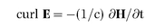
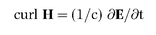
Great guns indeed. The essence of the theory is embodied in four equations which connect the six main quantities. They are now known to every physicist and electrical engineer as Maxwell’s equations. They are majestic mathematical statements, deep and subtle yet startlingly simple. So eloquent are they that one can get a sense of their beauty and power even without advanced mathematical training.

When the equations are applied to a point in empty space, the terms which represent the effects of electric charges and conduction currents are not needed⁶. The equations then become even simpler and take on a wonderful, stark symmetry; here they are⁷:

E is the electric force and H the magnetic force at our arbitrary point⁸. The bold lettering shows that they are vectors, having both strength and direction. ∂E/∂t and ∂H/∂t, also vectors, are the rates of change of E and H with time. The constant c acts as a kind of gear ratio between electric and magnetic forces—it is the ratio of the electromagnetic and electrostatic units of charge.

Leaving aside mathematical niceties, the equations can readily be interpreted in everyday terms. The terms ‘div’ (short for divergence) and ‘curl’ are ways of representing how the forces E and H vary in the space immediately surrounding the point. Div is a measure of the tendency of the force to be directed more outwards than inwards (div greater than zero), or more inwards than outwards (div less than zero). Curl, on the other hand, measures the tendency of the force to curl, or loop, around the point and gives the direction of the axis about which it curls.

• Equation (1) says that the electric force in a small region around our point has, on average, no inward or outward tendency. This implies that no electric charge is present.

• Equation (2) says the same for the magnetic force, implying that no single magnetic poles are present: they always come in north/south pairs in any case.

• The first two equations also imply the familiar laws for static fields: that the forces between electric charges and between magnetic poles vary inversely with the square of the distance separating them.

• Equation (3) says that when the magnetic force changes it wraps a circular electric force around itself. The minus sign means that the sense of the electric force is anticlockwise when viewed in the direction of the rate of change of the magnetic force.

• Equation (4) says that when the electric force changes it wraps a circular magnetic force around itself. The sense of the magnetic force is clockwise when viewed in the direction of the rate of change of the electric force.

• In equations (3) and (4) the constant c links the space variation (curl) of the magnetic force to the time variation (∂/∂t) of the electric force, and vice versa. It has the dimensions of a velocity and, as Maxwell rightly concluded, is the speed at which electromagnetic waves, including light, travel.

Equations (3) and (4) work together to give us these waves. We can get an idea of what happens simply by looking at the equations. A changing electric force wraps itself with a magnetic force; as that changes it wraps itself in a further layer of electric force and so on. Thus the changes in the combined field of electrical and magnetic forces spread out in a kind of continuous leapfrogging action.

In mathematical terms, equations (3) and (4) are two simultaneous differential equations with two unknowns. It is a simple matter to eliminate E and H in turn, giving one equation containing only H and another containing only E. In each case the solution turns out to be a form of equation known to represent a transverse wave travelling with speed c. The E and H waves always travel together: neither can exist alone. They vibrate at right angles to each other and are always in phase.

Thus any change in either the electrical or magnetic fields sends a combined transverse electromagnetic wave through space at a speed equal to the ratio of the electromagnetic and electrostatic units of charge. As we have seen, this ratio had been experimentally measured and, when put in the right units, was close to experimental measurements of the speed of light. James’ electromagnetic theory of light now no longer rested on a speculative model but was founded on the well-established principles of dynamics.

His system of equations worked with jewelled precision. Its construction had been an immense feat of sustained creative effort in three stages spread over 9 years. The whole route was paved with inspired innovations but from a historical perspective one crucial step stands out—the idea that electric currents exist in empty space. It is these displacement currents that give the equations their symmetry and make the waves possible. Without them the term ∂E/∂t in equation (4) becomes zero and the whole edifice crumbles.

Some accounts of the theory’s origin make no mention of the spinning cell model, or dismiss it as a makeshift contrivance which became irrelevant as soon as the dynamical theory appeared. In doing so they wrongly present Maxwell as a coldly cerebral mathematical genius. One can hardly dispute the epithet ‘genius’, but his thoughts were firmly rooted in the everyday physical world that all of us experience. The keystone of his beautiful theory, the displacement current, had its origin in the idea that the spinning cells in his construction-kit model could be springy.

James published A Dynamical Theory of the Electromagnetic Field in seven parts and introduced it at a presentation to the Royal Society in December 1864⁹. Most of his contemporaries were bemused. It was almost as if Einstein had popped out of a time machine to tell them about general relativity; they simply did not know what to make of it. Some thought that abandoning the mechanical model was a backward step; among these was William Thomson, who, for all his brilliance, never came close to understanding Maxwell’s theory.

One can understand these reactions. Not only was the theory ahead of its time but James was no evangelist and hedged his presentation with philosophical caution. He thought that his theory was probably right but could not be sure. No-one could until Heinrich Hertz produced and detected electromagnetic waves over 20 years later. The ‘great guns’ had been paraded but it would be a long while before they sounded.

It is almost impossible to overstate the importance of James’ achievement. The fact that its significance was but dimly recognised at the time makes it all the more remarkable. The theory encapsulated some of the most fundamental characteristics of the universe. Not only did it explain all known electromagnetic phenomena, it explained light and pointed to the existence of kinds of radiation not then dreamt of. Professor R. V. Jones was doing no more than representing the common opinion of later scientists when he described the theory as one of the greatest leaps ever achieved in human thought.

The authorities in King’s College had no more idea than anyone else of the immense significance of James’ electromagnetic theory. But they recognised the importance of his other research and experimental work and appreciated the kudos it brought to the university. They appointed a lecturer to help him with College duties. The first post-holder, George Smalley, left after a year for Australia and eventually became Astronomer Royal at Sydney. His successor was W. Grylls Adams, younger brother of John Couch Adams, in whose honour the Adams’ Prize had been founded. Even with this help James was finding it harder each year to fit in all the things he wanted to do. He and Katherine had by now a mass of data on colour vision which needed to be properly analysed and reported. There were ideas he wanted to pursue to extend his theory on gases. He saw a need for a substantial book on electricity and magnetism which would bring order to the subject and help newcomers. And he wanted more time at home, to make further improvements to the house and estate, and to play a more regular role as a leading person in local affairs. He decided to resign his chair so that he and Katherine could take up a settled life at Glenlair.

James handed over the professorship to Adams but agreed to help by returning to give evening lectures to the artisans during the following winter. They had been five good years in London. He had thrived on the variety: College lectures, home experiments on colour vision and gases, the experimental work on electrical standards for the British Association, and his two great papers on electromagnetism. It was wonderful to be able to walk to meetings at the Royal Society and Royal Institution, where he could enjoy the ready companionship of fellow scientists. But he was still a country boy at heart and he and Katherine loved their home. In the spring of 1865 they left their Kensington House for Glenlair.