13.8 Careful sample placement
A classic and effective family of techniques for variance reduction is based on the careful placement of samples in order to better capture the features of the integrand (or, more accurately, to be less likely to miss important features). These techniques are used extensively in pbrt. Indeed, one of the tasks of Samplers in Chapter 7 was to generate welldistributed samples for use by the integrators for just this reason, although at the time we offered only an intuitive sense of why this was worthwhile. Here we will justify that extra work in the context of Monte Carlo integration.
13.8.1 Stratified sampling
Stratified sampling was first introduced in Section 7.3, and we now have the tools to motivate its use. Stratified sampling works by subdividing the integration domain Λ into n nonoverlapping regions Λ1, Λ2, …, Λn. Each region is called a stratum, and they must completely cover the original domain:

To draw samples from Λ, we will draw ni samples from each Λi, according to densities pi inside each stratum. A simple example is supersampling a pixel. With stratified sampling, the area around a pixel is divided into a k × k grid, and a sample is drawn from each grid cell. This is better than taking k2 random samples, since the sample locations are less likely to clump together. Here we will show why this technique reduces variance.
Within a single stratum Λi, the Monte Carlo estimate is
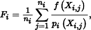
where Xi, j is the jth sample drawn from density pi. The overall estimate is  , where vi is the fractional volume of stratum i (vi ∈ (0, 1]).
The true value of the integrand in stratum i is
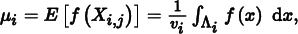
and the variance in this stratum is
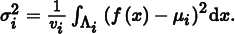
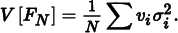
Thus, with ni samples in the stratum, the variance of the per-stratum estimator is σi2/ni. This shows that the variance of the overall estimator is

If we make the reasonable assumption that the number of samples ni is proportional to the volume vi, then we have ni = viN, and the variance of the overall estimator is
To compare this result to the variance without stratification, we note that choosing an unstratified sample is equivalent to choosing a random stratum I according to the discrete probability distribution defined by the volumes vi and then choosing a random sample X in ΛI. In this sense, X is chosen conditionally on I, so it can be shown using conditional probability that
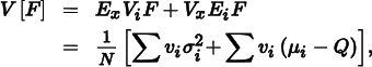
where Q is the mean of f over the whole domain Λ. See Veach (1997) for a derivation of this result.
There are two things to notice about this expression. First, we know that the right-hand sum must be nonnegative, since variance is always nonnegative. Second, it demonstrates that stratified sampling can never increase variance. In fact, stratification always reduces variance unless the right-hand sum is exactly 0. It can only be 0 when the function f has the same mean over each stratum Λi. In fact, for stratified sampling to work best, we would like to maximize the right-hand sum, so it is best to make the strata have means that are as unequal as possible. This explains why compact strata are desirable if one does not know anything about the function f. If the strata are wide, they will contain more variation and will have μi closer to the true mean Q.
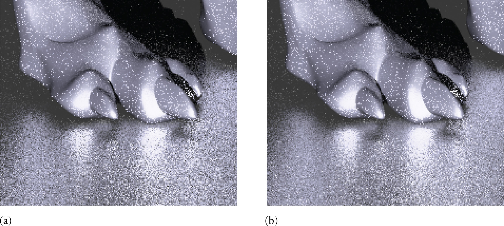
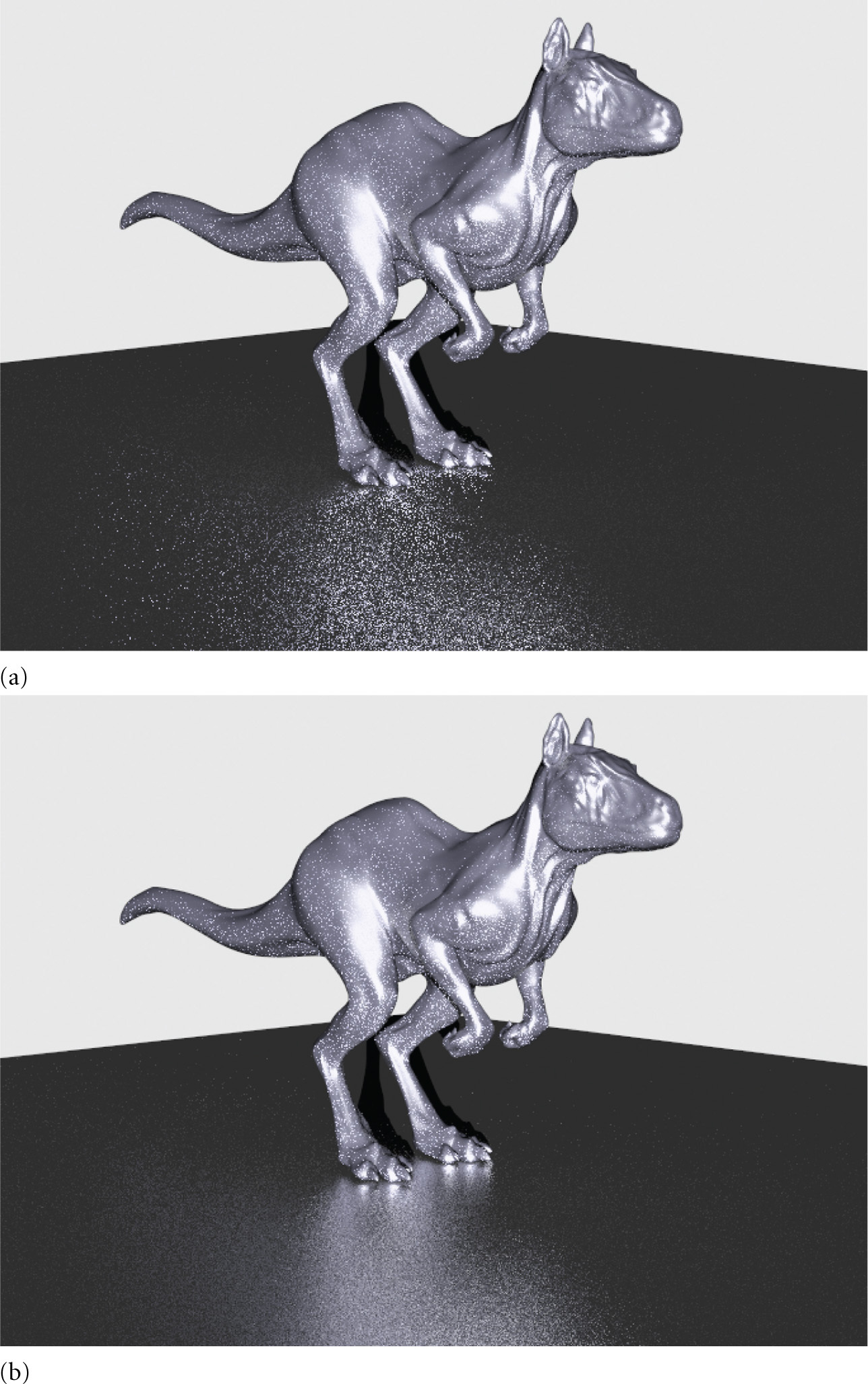
Figure 13.17 shows the effect of using stratified sampling versus a uniform random distribution for sampling ray directions for glossy reflection. There is a reasonable reduction in variance at essentially no cost in running time.
The main downside of stratified sampling is that it suffers from the same “curse of dimensionality” as standard numerical quadrature. Full stratification in D dimensions with S strata per dimension requires SD samples, which quickly becomes prohibitive. Fortunately, it is often possible to stratify some of the dimensions independently and then randomly associate samples from different dimensions, as was done in Section 7.3. Choosing which dimensions are stratified should be done in a way that stratifies dimensions that tend to be most highly correlated in their effect on the value of the integrand (Owen 1998). For example, for the direct lighting example in Section 13.7.1, it is far more effective to stratify the (x, y) pixel positions and to stratify the (θ, ϕ) ray direction— stratifying (x, θ) and (y, ϕ) would almost certainly be ineffective.
Another solution to the curse of dimensionality that has many of the same advantages of stratification is to use Latin hypercube sampling (also introduced in Section 7.3), which can generate any number of samples independent of the number of dimensions. Unfortunately, Latin hypercube sampling isn’t as effective as stratified sampling at reducing variance, especially as the number of samples taken becomes large. Nevertheless, Latin hypercube sampling is provably no worse than uniform random sampling and is often much better.
13.8.2 Quasi monte carlo
The low-discrepancy sampling techniques introduced in Chapter 7 are the foundation of a branch of Monte Carlo called quasi Monte Carlo. The key component of quasi–Monte Carlo techniques is that they replace the pseudo-random numbers used in standard Monte Carlo with low-discrepancy point sets generated by carefully designed deterministic algorithms.
The advantage of this approach is that for many integration problems, quasi–Monte Carlo techniques have asymptotically faster rates of convergence than methods based on standard Monte Carlo. Many of the techniques used in regular Monte Carlo algorithms can be shown to work equally well with quasi–random sample points, including importance sampling. Some others (e.g., rejection sampling) cannot. While the asymptotic convergence rates are not generally applicable to the discontinuous integrands in graphics because they depend on smoothness properties in the integrand, quasi Monte Carlo nevertheless generally performs better than regular Monte Carlo for these integrals in practice. The “Further Reading” section at the end of this chapter has more information about this topic.
In pbrt, we have generally glossed over the differences between these two approaches and have localized them in the Samplers in Chapter 7. This introduces the possibility of subtle errors if a Sampler generates quasi–random sample points that an Integrator then improperly uses as part of an implementation of an algorithm that is not suitable for quasi Monte Carlo. As long as Integrators only use these sample points for importance sampling or other techniques that are applicable in both approaches, this isn’t a problem.
13.8.3 Warping samples and distortion
When applying stratified sampling or low-discrepancy sampling to problems like choosing points on light sources for integration for area lighting, pbrt generates a set of samples (u1, u2) over the domain [0, 1)2 and then uses algorithms based on the transformation methods introduced in Sections 13.5 and 13.6 to map these samples to points on the light source. Implicit in this process is the expectation that the transformation to points on the light source will generally preserve the stratification properties of the samples from [0, 1)2—in other words, nearby samples should map to nearby positions on the surface of the light, and faraway samples should map to far-apart positions on the light. If the mapping does not preserve this property, then the benefits of stratification are lost.
Shirley’s square-to-circle mapping (Figure 13.13) preserves stratification more effectively than the straightforward mapping (Figure 13.12), which has less compact strata away from the center. This issue also explains why low-discrepancy sequences are generally more effective than stratified patterns in practice: they are more robust with respect to preserving their good distribution properties after being transformed to other domains. Figure 13.18 shows what happens when a set of 16 well-distributed sample points are transformed to be points on a skinny quadrilateral by scaling them to cover its surface; samples from a (0, 2)-sequence remain well distributed, but samples from a stratified pattern fare much less well.

13.9 Bias
Another approach to variance reduction is to introduce bias into the computation: sometimes knowingly computing an estimate that doesn’t actually have an expected value equal to the desired quantity can nonetheless lead to lower variance. An estimator is unbiased if its expected value is equal to the correct answer. If not, the difference
is the amount of bias.
Kalos and Whitlock (1986, pp. 36–37) gave the following example of how bias can sometimes be desirable. Consider the problem of computing an estimate of the mean value of a uniform distribution Xi ~ p over the interval from 0 to 1. One could use the estimator

or one could use the biased estimator

The first estimator is in fact unbiased but has variance with order O(N− 1). The second estimator’s expected value is
so it is biased, although its variance is O(N− 2), which is much better.
The pixel reconstruction method described in Section 7.8 can also be seen as a biased estimator. Considering pixel reconstruction as a Monte Carlo estimation problem, we’d like to compute an estimate of
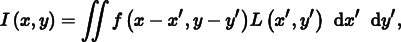
where I (x, y) is a final pixel value, f (x, y) is the pixel filter function (which we assume here to be normalized to integrate to 1), and L(x, y) is the image radiance function.
Assuming we have chosen image plane samples uniformly, all samples have the same probability density, which we will denote by pc. Thus, the unbiased Monte Carlo estimator of this equation is

This gives a different result from that of the pixel filtering equation we used previously, Equation (7.12), which was
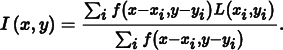
Yet, the biased estimator is preferable in practice because it gives a result with less variance. For example, if all radiance values L(xi, yi) have a value of 1, the biased estimator will always reconstruct an image where all pixel values are exactly 1—clearly a desirable property. However, the unbiased estimator will reconstruct pixel values that are not all 1, since the sum
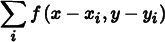
will generally not be equal to pc and thus will have a different value due to variation in the filter function depending on the particular (xi, yi) sample positions used for the pixel. Thus, the variance due to this effect leads to an undesirable result in the final image. Even for more complex images, the variance that would be introduced by the unbiased estimator is a more objectionable artifact than the bias from Equation (7.12).
13.10 Importance sampling
Importance sampling is a powerful variance reduction technique that exploits the fact that the Monte Carlo estimator
converges more quickly if the samples are taken from a distribution p(x) that is similar to the function f (x) in the integrand. The basic idea is that by concentrating work where the value of the integrand is relatively high, an accurate estimate is computed more efficiently (Figure 13.19).
For example, suppose we are evaluating the scattering equation, Equation (5.9). Consider what happens when this integral is estimated; if a direction is randomly sampled that is nearly perpendicular to the surface normal, the cosine term will be close to 0. All the expense of evaluating the BSDF and tracing a ray to find the incoming radiance at that sample location will be essentially wasted, as the contribution to the final result will be minuscule. In general, we would be better served if we sampled directions in a way that reduced the likelihood of choosing directions near the horizon. More generally, if directions are sampled from distributions that match other factors of the integrand (the BSDF, the incoming illumination distribution, etc.), efficiency is similarly improved.
As long as the random variables are sampled from a probability distribution that is similar in shape to the integrand, variance is reduced. We will not provide a rigorous proof of this fact but will instead present an informal and intuitive argument. Suppose we’re trying to use Monte Carlo techniques to evaluate some integral ∫ f (x) dx. Since we have freedom in choosing a sampling distribution, consider the effect of using a distribution p(x) ∝ f (x), or p(x) = cf (x). It is trivial to show that normalization forces
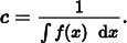
Finding such a PDF requires that we know the value of the integral, which is what we were trying to estimate in the first place. Nonetheless, for the purposes of this example, if we could sample from this distribution, each estimate would have the value
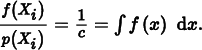
Since c is a constant, each estimate has the same value, and the variance is zero! Of course, this is ludicrous since we wouldn’t bother using Monte Carlo if we could integrate f directly. However, if a density p(x) can be found that is similar in shape to f (x), variance decreases.
Importance sampling can increase variance if a poorly chosen distribution is used. To understand the effect of sampling from a PDF that is a poor match for the integrand, consider using the distribution

to compute the estimate of ∫ f (x) dx where
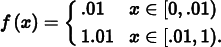
By construction, the value of the integral is one, yet using p(x) to draw samples to compute a Monte Carlo estimate will give a terrible result: almost all of the samples will be in the range [0, .01), where the estimator has the value f (x)/p(x) ≈ 0.0001. For any estimate where none of the samples ends up being outside of this range, the result will be very inaccurate, almost 10,000 times smaller than it should be. Even worse is the case where some samples do end up being taken in the range [.01, 1). This will happen rarely, but when it does, we have the combination of a relatively high value of the integrand and a relatively low value of the PDF, f (x)/p(x) = 101. A large number of samples would be necessary to balance out these extremes to reduce variance enough to get a result close to the actual value, 1.
Fortunately, it’s not too hard to find good sampling distributions for importance sampling for many integration problems in graphics. As we implement Integrators in the next three chapters, we will derive a variety of sampling distributions for BSDFs, lights, cameras, and participating media. In many cases, the integrand is the product of more than one function. It can be difficult to construct a PDF that is similar to the complete product, but finding one that is similar to one of the multiplicands is still helpful.
In practice, importance sampling is one of the most frequently used variance reduction techniques in rendering, since it is easy to apply and is very effective when good sampling distributions are used.
13.10.1 Multiple importance sampling
Monte Carlo provides tools to estimate integrals of the form ∫ f (x) dx. However, we are frequently faced with integrals that are the product of two or more functions: ∫ f (x)g(x) dx. If we have an importance sampling strategy for f (x) and a strategy for g(x), which should we use? (Assume that we are not able to combine the two sampling strategies to compute a PDF that is proportional to the product f (x)g(x) that can itself be sampled easily.) As discussed above, a bad choice of sampling distribution can be much worse than just using a uniform distribution.
For example, consider the problem of evaluating direct lighting integrals of the form

If we were to perform importance sampling to estimate this integral according to distributions based on either Ld or fr, one of these two will often perform poorly.
Consider a near-mirror BRDF illuminated by an area light where Ld’s distribution is used to draw samples. Because the BRDF is almost a mirror, the value of the integrand will be close to 0 at all ωi directions except those around the perfect specular reflection direction. This means that almost all of the directions sampled by Ld will have 0 contribution, and variance will be quite high. Even worse, as the light source grows large and a larger set of directions is potentially sampled, the value of the PDF decreases, so for the rare directions where the BRDF is non-0 for the sampled direction we will have a large integrand value being divided by a small PDF value. While sampling from the BRDF’s distribution would be a much better approach to this particular case, for diffuse or glossy BRDFs and small light sources, sampling from the BRDF’s distribution can similarly lead to much higher variance than sampling from the light’s distribution.
Unfortunately, the obvious solution of taking some samples from each distribution and averaging the two estimators is little better. Because the variance is additive in this case, this approach doesn’t help—once variance has crept into an estimator, we can’t eliminate it by adding it to another estimator even if it itself has low variance.
Multiple importance sampling (MIS) addresses exactly this issue, with a simple and easy-to-implement technique. The basic idea is that, when estimating an integral, we should draw samples from multiple sampling distributions, chosen in the hope that at least one of them will match the shape of the integrand reasonably well, even if we don’t know which one this will be. MIS provides a method to weight the samples from each technique that can eliminate large variance spikes due to mismatches between the integrand’s value and the sampling density. Specialized sampling routines that only account for unusual special cases are even encouraged, as they reduce variance when those cases occur, with relatively little cost in general. See Figure 14.13 in Chapter 14 to see the reduction in variance from using MIS to compute reflection from direct illumination compared to sampling either just the BSDF or the light’s distribution by itself.
If two sampling distributions pf and pg are used to estimate the value of ∫ f (x)g(x) dx, the new Monte Carlo estimator given by MIS is
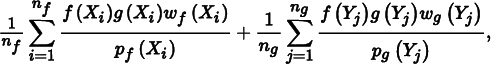
where nf is the number of samples taken from the pf distribution method, ng is the number of samples taken from pg, and wf and wg are special weighting functions chosen such that the expected value of this estimator is the value of the integral of f (x)g(x).
The weighting functions take into account all of the different ways that a sample Xi or Yj could have been generated, rather than just the particular one that was actually used. A good choice for this weighting function is the balance heuristic:

The balance heuristic is a provably good way to weight samples to reduce variance.
Consider the effect of this term for the case where a sample X has been drawn from the pf distribution at a point where the value pf(X) is relatively low. Assuming that pf is a good match for the shape of f (x), then the value of f (X) will also be relatively low. But suppose that g(X) has a relatively high value. The standard importance sampling estimate

will have a very large value due to pf (X) being small, and we will have high variance. With the balance heuristic, the contribution of X will be
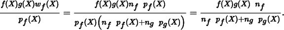
As long as pg’s distribution is a reasonable match for g(x), then the denominator won’t be too small thanks to the ngpg(X) term, and the huge variance spike is eliminated, even though X was sampled from a distribution that was in fact a poor match for the integrand. The fact that another distribution will also be used to generate samples and that this new distribution will likely find a large value of the integrand at X are brought together in the weighting term to reduce the variance problem.
Here we provide an implementation of the balance heuristic for the specific case of two distributions pf and pg. We will not need a more general multidistribution case in pbrt.
〈Sampling Inline Functions〉 + ≡
inline Float BalanceHeuristic(int nf, Float fPdf, int ng, Float gPdf) {
return (nf * fPdf) / (nf * fPdf + ng * gPdf);
In practice, the power heuristic often reduces variance even further. For an exponent β, the power heuristic is
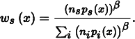
Veach determined empirically that β = 2 is a good value. We have β = 2 hard-coded into the implementation here.
〈Sampling Inline Functions〉 + ≡
inline Float PowerHeuristic(int nf, Float fPdf, int ng, Float gPdf) {
Float f = nf * fPdf, g = ng * gPdf;
return (f * f) / (f * f + g * g);
Further reading
Many books have been written on Monte Carlo integration. Hammersley and Handscomb (1964), Spanier and Gelbard (1969), and Kalos and Whitlock (1986) are classic references. More recent books on the topic include those by Fishman (1996) and Liu (2001). Chib and Greenberg (1995) have written an approachable but rigorous introduction to the Metropolis algorithm. The Monte Carlo and Quasi Monte Carlo Web site is a useful gateway to recent work in the field (www.mcqmc.org).
Good general references about Monte Carlo and its application to computer graphics are the theses by Lafortune (1996) and Veach (1997). Dutré’s Global Illumination Compendium (2003) also has much useful information related to this topic. The course notes from the Monte Carlo ray-tracing course at SIGGRAPH have a wealth of practical information (Jensen et al. 2001a, 2003).
The square to disk mapping was described by Shirley and Chiu (1997). The implementation here benefits by observations by Cline and “franz” that the logic could be simplified considerably from the original algorithm (Shirley 2011). Marques et al. (2013) note that well-distributed samples on [0, 1)2 still suffer some distortion when they are mapped to the sphere of directions and show how to generate low-discrepancy samples on the unit sphere.
Steigleder and McCool (2003) described an alternative to the multidimensional sampling approach from Section 13.6.7: they linearized 2D and higher dimensional domains into 1D using a Hilbert curve and then sampled using 1D samples over the 1D domain. This leads to a simpler implementation that still maintains desirable stratification properties of the sampling distribution, thanks to the spatial coherence preserving properties of the Hilbert curve.
Lawrence et al. (2005) described an adaptive representation for CDFs, where the CDF is approximated with a piecewise linear function with fewer, but irregularly spaced, vertices compared to the complete CDF. This approach can substantially reduce storage requirements and improve lookup efficiency, taking advantage of the fact that large ranges of the CDF may be efficiently approximated with a single linear function.
Cline et al. (2009) observed that the time spent in binary searches for sampling from precomputed distributions (like Distribution1D does) can take a meaningful amount of execution time. (Indeed, pbrt spends nearly 7% of the time when rendering the car scene lit by an InfiniteAreaLight in the Distribution1D::SampleContinuous() method, which is used by InfiniteAreaLight::Sample_Li().) They presented two improved methods for doing this sort of search: the first stores a lookup table with n integer values, indexed by ⌊nξ⌋, which gives the first entry in the CDF array that is less than or equal to ξ. Starting a linear search from this offset in the CDF array can be much more efficient than a complete binary search over the entire array. They also presented a method based on approximating the inverse CDF as a piecewise linear function of ξ and thus enabling constant-time lookups at a cost of some accuracy (and thus some additional variance).
The alias method is a technique that makes it possible to sample from discrete distributions in O(1) time (Walker 1974, 1977); this is much better than the O(log n) of the Distribution1D class when it is used for sampling discrete distributions. The downside of this approach is that it does not preserve sample stratification. See Schwarz’s writeup (2011) for information about implementing this approach well.
Arithmetic coding offers another interesting way to approach sampling from distributions (MacKay 2003, p. 118; Piponi 2012). If we have a discrete set of probabilities we’d like to generate samples from, one way to approach the problem is to encode the CDF as a binary tree where each node splits the [0, 1) interval at some point and where, given a random sample ξ, we determine which sample value it corresponds to by traversing the tree until we reach the leaf node for its sample value. Ideally, we’d like to have leaf nodes that represent higher probabilities be higher up in the tree, so that it takes fewer traversal steps to find them (and thus, those more frequently generated samples are found more quickly). Looking at the problem from this perspective, it can be shown that the optimal structure of such a tree is given by Huffman coding, which is normally used for compression.
Mitchell (1996b) wrote a paper that investigates the effects of stratification for integration problems in graphics (including the 2D problem of pixel antialiasing). In particular, he investigated the connection between the complexity of the function being integrated and the effect of stratification. In general, the smoother or simpler the function, the more stratification helps: for pixels with smooth variation over their areas or with just a few edges passing through them, stratification helps substantially, but as the complexity in a pixel is increased, the gain from stratification is reduced. Nevertheless, because stratification never increases variance, there’s no reason not to do it.
Starting with Durand et al.’s work (2005), a number of researchers have approached the analysis of light transport and variance from Monte Carlo integration for rendering using Fourier analysis. See Pilleboue et al.’s paper (2015) for recent work in this area, including references to previous work. Among other results, they show that Poisson disk patterns give higher variance than simple jittered patterns. They found that the blue noise pattern of de Goes et al. (2012) was fairly effective. Other work in this area includes the paper by Subr and Kautz (2013).
Multiple importance sampling was developed by Veach and Guibas (Veach and Guibas 1995; Veach 1997). Normally, a pre-determined number of samples are taken using each sampling technique; see Pajot et al. (2011) and Lu et al. (2013) for approaches to adaptively distributing the samples over strategies in an effort to reduce variance by choosing those that are the best match to the integrand.
Exercises
 13.1 Write a program that compares Monte Carlo and one or more alternative numerical integration techniques. Structure this program so that it is easy to replace the particular function being integrated. Verify that the different techniques compute the same result (given a sufficient number of samples for each of them). Modify your program so that it draws samples from distributions other than the uniform distribution for the Monte Carlo estimate, and verify that it still computes the correct result when the correct estimator, Equation (13.3), is used. (Make sure that any alternative distributions you use have nonzero probability of choosing any value of x where f (x) > 0.)
 13.2 Write a program that computes Monte Carlo estimates of the integral of a given function. Compute an estimate of the variance of the estimates by taking a series of trials and using Equation (13.2) to compute variance. Demonstrate numerically that variance decreases at a rate of
  .
.
13.3 The depth-of-field code for the ProjectiveCamera in Section 6.2.3 uses the ConcentricSampleDisk() function to generate samples on the circular lens, since this function gives less distortion than UniformSampleDisk(). Try replacing it with UniformSampleDisk(), and measure the difference in image quality. For example, you might want to compare the error in images from using each approach and a relatively low number of samples to a highly sampled reference image.
Does ConcentricSampleDisk() in fact give less error in practice? Does it make a difference if a relatively simple scene is being rendered versus a very complex scene?
13.4 Modify the Distribution1D implementation to use the adaptive CDF representation described by Lawrence et al. (2005), and experiment with how much more compact the CDF representation can be made without causing image artifacts. (Good test scenes include those that use InfiniteAreaLights, which use the Distribution2D and, thus, Distribution1D for sampling.) Can you measure an improvement in rendering speed due to more efficient searches through the approximated CDF?
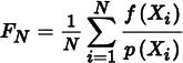
 13.5 One useful technique not discussed in this chapter is the idea of adaptive density distribution functions that dynamically change the sampling distribution as samples are taken and information is available about the integrand’s actual distribution as a result of evaluating the values of these samples. The standard Monte Carlo estimator can be written to work with a nonuniform distribution of random numbers used in a transformation method to generate samples Xi,

just like the transformation from one sampling density to another. This leads to a useful sampling technique, where an algorithm can track which samples ξi were effective at finding large values of f (x) and which weren’t and then adjusts probabilities toward the effective ones (Booth 1986). A straightforward implementation would be to split [0, 1] into bins of fixed width, track the average value of the integrand in each bin, and use this to change the distribution of ξi samples.
Investigate data structures and algorithms that support such sampling approaches and choose a sampling problem in pbrt to apply them to. Measure how well this approach works for the problem you selected. One difficulty with methods like this is that different parts of the sampling domain will be the most effective at different times in different parts of the scene. For example, trying to adaptively change the sampling density of points over the surface of an area light source has to contend with the fact that, at different parts of the scene, different parts of the area light may be visible and thus be the important areas. You may find it useful to read Cline et al.’s paper (2008) on this topic.