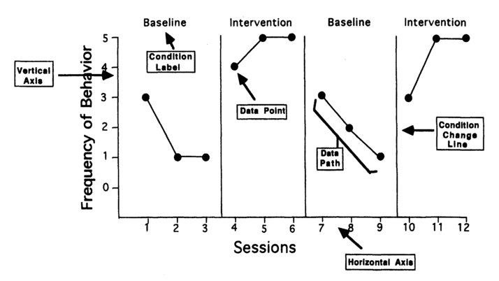
Figure 8.1 Hypothetical example of a single-case design graph depicting the major features of graphic display.
In Chapter 7 we outlined the protocols used to identify, operationalize, and assess target behaviors over time. Applied behavior analysis is also characterized by a series of experimental techniques known as single-case designs. These experimental techniques are used to determine if changes in the dependent variable or target behavior can be attributed to the independent variable or treatment. Single-case research designs are therefore used to examine whether treatment applications actually cause the desired change in the target behavior. In other words, these experimental techniques examine the functional relationships between changes in the environment and changes in the target behavior. Single-case designs are also unique in their ability to examine causally such functional relations with individual cases (i.e., one person) in addition to groups of individuals. Applied behavior analysts use several different types of single-case designs. These designs can also be combined to tease out complex maintaining variables (Higgins-Hains & Baer, 1989). Despite the variety of single-case designs, they are all based on the same set of fundamental premises and techniques.
All single-case methods are designed to eliminate threats to internal validity. Internal validity refers to the extent to which a research method can rule out alternative explanations for changes in the target behavior. The application of a treatment does not occur in a vacuum. There are other dynamic environmental conditions that are constantly changing and influencing a person's behavior. These other environmental influences may pose as alternative explanations for changes in the target behavior above and beyond the treatment application, and are thus described as threats to internal validity. Several categories of threats to internal validity have been described in the literature (see Kazdin, 1982). History and maturation are two such threats. History refers to any environmental event that occurs concurrently with the experiment or intervention and could account for similar results as those attributed to the intervention. History encapsulates a myriad of possible idiosyncratic environmental influences for a given case (for example, negative interactions with individuals, adverse environmental conditions etc.). Maturation refers to any changes in the target behavior over time that may result from processes within the person. These personal processes may include the health of the individual, boredom, or aging. For example, allergy symptoms have been shown to have a significant influence on treatment applications (Kennedy & Meyer, 1996). Single-case research methods are designed to rule out these and other threats to internal validity. The process by which each design accomplishes this will be discussed in later sections of this chapter.
External validity refers to the ability to extend the findings of an experiment to other persons, settings, and clinical syndromes with confidence. Some applied researchers have proposed that external validity should take precedence over internal validity when designing applied research studies (Kazdin, 1982). While such a proposition is probably incorrect, because demonstrating internal validity is a necessary prerequisite for demonstrating external validity, it emphasizes the importance of external validity in applied research.
Aspects of the experimental preparation that may limit the generality of findings are referred to as threats to external validity. There are numerous threats to the external validity of an experiment (see Cook & Campbell, 1979; Kazdin, 1982). Two of these threats include generality across settings, responses and time; and multiple treatment interference. This former threat to external validity proposes that, for any experimental manipulation, the results may be restricted to the particular target behaviors within the immediate context of the intervention and during the time of intervention only. Such threats to external validity can be minimized by using particular research design options (such as multiple baseline designs, discussed below) that can systematically examine these issues of generalization within the context of a given experimental preparation. Multiple treatment interference occurs when two or more treatments are evaluated with a given target behavior. When treatments are compared there is always the possibility that the effects of one treatment are confounded by experience with a previous treatment. In other words, the sequence of treatment administration may influence the performance of the individual. Strong conclusions about the influence of any one treatment cannot be made from such an experimental preparation. Extended single-case experimental preparations can be used to tease the relative effects of two or more treatments (see Barlow & Hersen, 1984) but such research designs may be impractical in most applied settings (Higgins-Hains & Baer, 1989).
Single-case research designs typically use graphic display to present an ongoing visual representation of each assessment session. Graphic display is a simple visual method for organizing, interpreting, and communicating findings in the field of applied behavior analysis. While many forms of graphic display can be used the majority of applied research results are presented in simple line graphs or frequency polygons. A line graph is a two dimensional plane formed by the intersection of two perpendicular lines. Each data point plotted on a line graph represents a relationship between the two properties described by the intersecting lines. In applied behavior analysis the line graph represents changes in the dependent variable (e.g., frequency, rate, or percentage of the target behavior per session) relative to a specific point in time and/or treatment (independent) variable.
An example of a line graph is presented in Figure 8.1. The major features of this graph include the horizontal and vertical axes, condition change lines, condition labels, data points and data paths. The horizontal axis represents the passage of time (consecutive sessions) and the different levels of the independent variable (baseline and intervention). The vertical axis represents values of the dependent variable. The condition change lines represent that point in time when the levels of the independent variable were systematically changed. Condition labels are brief descriptions of the experimental conditions in effect during each phase of the study. Each data point represents the occurrence of the target behavior during a session under a given experimental condition. Connecting the data points with a straight line under a given experimental condition creates a data path. A data path represents the relationship between the independent and dependent variables and is of primary interest when interpreting graphed data (see below).
The use of graphic display to examine functional relations has a number of inherent benefits. First, as a judgmental aid, it is easy to use and easy to learn (Michael, 1974). Second, it allows the therapist to have an ongoing access to a complete record of the participant's behavior. Behavior change can therefore be evaluated continuously. If the treatment is not proving effective then the therapist can alter the treatment protocol and subsequently evaluate these changes on an ongoing basis. Third, visual analysis provides a stringent method for evaluating the effectiveness of behavior change programs (Baer, 1977). Finally, graphic display provides an objective assessment of the effectiveness of the independent variable. These displays allow for independent judgements on the meaning and significance of behavior change strategies.

Figure 8.1 Hypothetical example of a single-case design graph depicting the major features of graphic display.
The primary method of analysis with all single-case research designs is a visual interpretation of graphic displays. There are several properties of graphic displays that are important to consider when making a determination of the effects of the treatment variable on the target behavior or when deciding to change from one condition (e.g., baseline) to another (e.g., treatment) during an applied behavioral intervention. These properties include number of data points, overall stability of the data, data levels, and data trends.
It is important to collect a sufficient number of data points in order to provide a believable estimate of the performance of the target behavior under a given experimental condition. There are no hard and fast rules about the number of data points that should be collected under a given experimental condition. Sidman (1960) suggests that at least three measures of the target behavior should be collected per experimental condition. This is an optimal suggestion if the data path is stable (see below) and the nature of the target behavior allows for multiple assessments under baseline and intervention conditions. For example, if the target behavior is dangerous to the client or others (for example, when it involves aggression) it may be unethical to conduct extended assessments under baseline conditions (that is, when the treatment variable is not present).
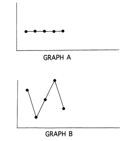
Figure 8.2 Hypothetical example of a stable data path (Graph A) and variable data points (Graph B).
Stability refers to a lack of variability in the data under a given experimental condition. In Figure 8.2 it is clear that Graph A presents a stable data path whereas the data in Graph B are variable. It is unusual in applied research to achieve prefect stability of data as illustrated in Graph A. Tawney and Gast (1984) provide a general rule for determining stability of data within experimental conditions. We may concluded that there is stability if 80-90% of the data points within a condition fall within a 15% range of the mean level of all data points for that particular experimental condition. It is unusual for applied researchers to use such mathematical formulae. If stability is not obvious from a visual examination of the data then it may be prudent to identify those environmental stimuli that are causing such variability in the data set. This further analysis may yield additional functional variables that may need to be manipulated to achieve successful intervention results.
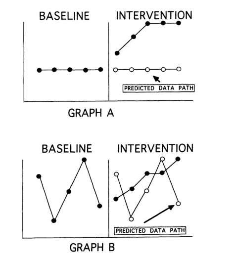
Figure 8.3 Stable baseline data (Graph A) allow for a clear interpretation of the effectiveness of treatment in the intervention phase. When baseline data are variable (Graph B) it becomes difficult to evaluate the effects of the treatment in the intervention phase.
Stability of data within a given experimental condition is also important because the data path serves a predictive function for interpreting data within the subsequent experimental condition. A stable data path within a given experimental condition allows the therapist to infer that if that experimental condition was continued over time, a similar data pattern would emerge (see Figure 8.3). The effects of the subsequent condition are determined by comparing the observed data (i.e., the actual data obtained when the experimental conditions were changed) with the predicted data from the previous condition. Stability of predicted data therefore allows for a clearer interpretation of the effect of subsequent experimental conditions on the target behavior. In Figure 8.3 the predicted data paths for a stable data set (Graph A) and variable data set (Graph B) are plotted. It is obvious that the effects of the intervention can be more clearly interpreted by comparing predicted with observed data for Graph A than for Graph B.

Figure 8.4 There is a clear change in level between the last data point of the baseline phase and the first data point of the intervention phase in Graph A. There is no change in level between the baseline and intervention in Graph B until the third data point of the intervention phase. This delayed change in level when treatment is applied may mean that something other than the treatment caused a change in the target behavior.
Level can be defined as the value of a behavioral measure or group of measures on the vertical axis of a line graph. Level can be used to describe overall performance within an experimental condition or between experimental conditions. Typically, the levels of performance within and between conditions are analyzed visually by the therapist. However, a mean level can also be calculated for each condition. Stability and level are inextricably linked in the visual analysis of data. If extreme variability exists in the data paths then a visual examination of level within and between conditions may be impossible. Level is also used to examine the difference between the last data point of a condition and the first data point of the following experimental condition. If there is an obvious level change in behavior at that point in time when the new experimental condition is implemented then the therapist can more confidently infer that the change in behavior is due to a change in the experimental condition. In Figure 8.4 (Graph A) there is an obvious level change between conditions when the intervention is implemented. In Graph B the level change during the intervention phase does not occur until the third data point. It may be the case for Graph B that something other than or in addition to the intervention causes a level change in behavior from the third data point onwards.
Trend can be defined as the overall direction taken by a data path. Trends can be described as increasing, decreasing, or zero. A stable data path represents a zero trend, increasing and decreasing trends can be problematic for interpreting data. If, for example, a therapist wants to increase responding, an increasing trend in the baseline data path may make interpretation of the effects of the intervention difficult (see Figure 8.5, Graph A). This logic also holds for decreasing trends (see Figure 8.5, Graph B). It is advisable in such cases to withhold the intervention until the data path stabilizes under baseline conditions or until the behavior reaches the desired goal. In some applied situations it may be impractical (the presence of the therapist may be time-limited) or unethical (the behavior may be dangerous to self or others) to withhold treatment for extended periods. In these situations experimental control may need to be sacrificed in order to achieve the desired behavioral outcomes. Under some circumstances a trend in data may not interfere with the interpretation of the subsequent experimental condition. This is true for situations where the trend under a given experimental condition is going in the opposite direction that would be predicted when the subsequent experimental condition is implemented (see Figure 8.5, Graph C).
Withdrawal or ABAB designs represent a series of experimental arrangements whereby selected conditions are systematically presented and withdrawn over time. This design typically consists of two phases, a baseline or A phase and an intervention or B phase that are replicated (hence the ABAB notation). The design begins with an assessment of behavior under baseline conditions. Once the target behavior stabilizes
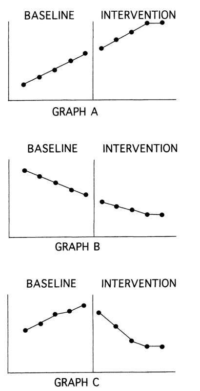
Figure 8.5 An increasing or decreasing trend in baseline data paths can be problematic if the subsequent intervention is designed to increase (Graph A) or decrease (Graph B) the target behavior respectively. A trend in the baseline data path may not interfere with an interpretation of an intervention effect if the treatment is designed to change the trend in the opposite direction (Graph C).
under baseline conditions the intervention condition is implemented. The intervention condition is continued until the target behavior reaches a stable level or diverges from the level predicted from the baseline data. At this point the intervention is withdrawn and the baseline condition is replicated until stability is achieved. Finally the intervention condition is once again implemented. Experimental control is achieved when there is a visible difference between the data paths in the A and B phases and this difference is again achieved in the A and B phase replications.
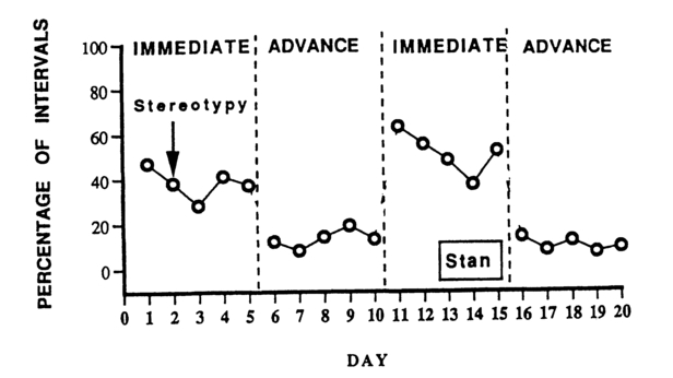
Figure 8.6 Percentage of intervals of stereotypy during transition between work activities for a man with autism. This ABAB design compared immediate requests with an advanced notice procedure to change work tasks (Tustin, 1995).
Examples of the use of ABAB designs abound in the applied literature. In a recent study, Tustin (1995) used a withdrawal design to compare the effects of two methods of requesting activity change on the stereotypic behavior of an adult with autism. Persons with autism tend to engage in stereotypic behavior (e.g., body rocking, hand flapping) when asked to change from one activity to another. An immediate request for change involved the work supervisor presenting new materials, removing present materials, and instructing the new task. An advanced notice request involved much the same behavior by the work supervisor with the exception that the activities for the new task were placed in view of the participant 2 minutes prior to the request to change tasks. Stereotypy was measured using a partial interval recording procedure, and the influence of the two requesting conditions was examined over a 20-day period. The results of the investigation are presented in Figure 8.6. The immediate request condition produced a relatively stable pattern of responding during the first five days of the assessment. The advanced notice request condition produced an immediate reduction in stereotypy and stable responding over the next five days. These results were again replicated in an immediate and advanced notice condition. The results of the ABAB design clearly show the effectiveness of the advanced notice requesting technique in reducing stereotypy when transitioning between tasks for this participant.
In another example, Friman and Vollmer (1995) examined the effectiveness of a urine alarm to treat chronic diurnal enuresis for a young female diagnosed with depression and attention deficit hyperactivity disorder. Wetness was examined twice a day under baseline conditions (i.e., no intervention in place) for a 5-week period. The participant was then fitted with a moisture sensitive alarm for 4 weeks. The baseline and alarm conditions were then replicated. The results of this study are presented in Figure 8.7. During the initial baseline assessment the participant had wetting accidents each day. Once the alarm intervention was implemented the wetting accidents decreased dramatically to zero levels. When the alarm was removed (second baseline condition) the number of wetting accidents increased again but did not return to the same level observed during the initial baseline condition. Once the alarm was reinstated the number of accidents decreased to zero with maintenance of these results for up to 6 months.
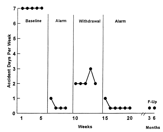
Figure 8.7 Number of accident days per week for an adolescent girl with diurnal enuresis (Friman & Vollmer, 1995).

Figure 8.8 The number of self-identified designated drivers per evening during weekend evenings in a college campus bar. The mean number of self-identified designated drivers in each phase for the design is also included in the graph (Brigham, Meier, & Goodner, 1995).
Finally, Brigham, Meier, and Goodner (1995) examined the influence of a prompts-with-incentives program to increase designated drivers in a local bar (that is, people who would not drink alcohol that night, and thus be fit to drive). The intervention consisted of a series of posters displayed around the bar that indicated the availability of free non-alcoholic beverages (beer, wine, coffee, juice etc.) for those patrons who identified themselves as designated drivers. These posters were not displayed during baseline conditions. The dependent measure consisted of those bar patrons who identified themselves as designated drivers to the bar staff (and received free beverages) and subsequently drove a vehicle away from the bar. The intervention was conducted on Friday and Saturday nights and used an ABAB design to evaluate its effectiveness (see Figure 8.8). Overall, the results of this study indicate that there is an increase in designated drivers under the intervention conditions. However, these results are not as clear as those of the other two studies described. For example, there is not a clear visual differentiation or separation between the data paths under baseline and intervention conditions. Additionally, there is no immediate level change between the last data point of the second baseline phase and the first data point of the second intervention phase. Data paths during both intervention conditions did not achieve stability, however there is a data trend in the direction expected by the intervention (the intervention is expected to increase designated drivers). Based on these visual analyses of the data, the positive effects of the intervention must be interpreted with caution.
Withdrawal designs can be adapted to answer additional research questions (other than the comparative effect of a baseline and an intervention on a dependent variable) and to examine causality where the traditional design strategy would be inappropriate. For example, the ABAB design has been used to examine the influence of a baseline and intervention condition on multiple and simultaneous data paths. Kern, Wacker, Mace, Falk, Dunlap, and Kromrey (1995) evaluated the effects of a seif-evaluation program to improve peer interactions of students with emotional and behavior disorders. The experimental protocol used by Kern et al., (1995) included a withdrawal design that simultaneously measured appropriate and inappropriate interactions of the targeted students with their peers during observation sessions.
Withdrawal designs can also be used to examine the effectiveness of more than one treatment. Occasionally the initial treatment (in the B phase) may fail to achieve sufficient change in the target behavior. In such situations an alternative treatment may be examined. This type of design is typically described as an ABABCBC design. Such a design incorporates a systematic comparison of the first treatment with baseline (ABAB) and the first treatment with the second treatment (BCBC). The results of such treatment comparisons must be interpreted with caution as they do not rule out sequence effects (that is, the effectiveness of C may be influenced by the fact that it was preceded by B). Jason and Liotta (1982) used an ABABCBC design to compare the effects of sign prompting alone and sign prompting plus verbal prompting on the reduction of smoking at a university cafeteria. Figure 8.9 shows the results of this study. The sign prompting alone did not produce a significant change in the number of smokers or the number of minutes smoked during observation sessions. When sign prompting was combined with verbal prompting there was a significant reduction in the target behaviors.
The sequence of A and B conditions in a withdrawal design can also be reversed, to BABA, without compromising the experimental validity of this
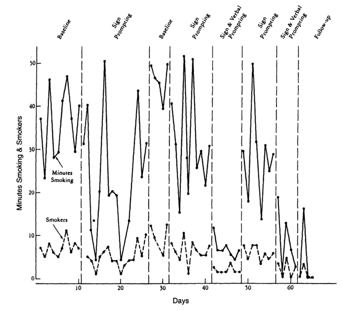
Figure 8.9 An example of an ABABCBC design. This research examined the influence of two interventions (sign prompting and sign plus verbal prompting) on minutes smoking and number of smokers in a university cafeteria. The first intervention (sign prompting alone) was not successful (see ABAB phases of the design). Sign prompting was then compared with sign plus verbal prompting (see BCBC phases of the design) (Jason & Liotta, 1982).
design option. In other words, once the target behavior is clearly identified the intervention can be implemented immediately. Once the data path achieves stability in the B phase the intervention can then be withdrawn. These phases can then be replicated. For applied intervention purposes the design can be completed with a third replication of the intervention phase (i.e., BABAB). Several authors have suggested such a design option for behavior that is in need of immediate intervention (behavior that is of danger to self or others) (Cooper, Heron, & Heward, 1987; Tawney & Gast, 1984). However, this research protocol would be inappropriate in such cases as it continues to require a return to pre-intervention conditions. Alternative design strategies that do not require extended baseline assessments (such as multielement designs) would be more efficient and ethically appropriate in such cases.
Withdrawal designs have been described as the most rigorous of the single-case research options for ruling out threats to internal validity (Kazdin, 1994). The withdrawal design is a very effective means of examining the effects of a treatment on selected target behaviors. There are several issues that must be considered however, before selecting to use the withdrawal design above one of the other design options. This design option demonstrates experimental control by systematically applying and removing the treatment variables. The purposeful withdrawal of treatment is seldom a preferable option in clinical practice. There may therefore be ethical reasons (as in the example of behavior that is dangerous to self or others) for not using such a design option. Certain types of behaviors (e.g., social skills) might be expected to maintain or at least to continue to be performed above initial baseline levels after the intervention is withdrawn. If the target behavior does not revert to the initial baseline levels with the withdrawal of treatment (i.e., second A phase) then experimental control is lost. It is therefore important to consider whether the target behavior would be sensitive to the changing contingencies of an ABAB design. Again, alternative designs can be chosen if this is a potential issue.
The multiple baseline design is an experimental preparation whereby the independent variable is sequentially applied to a minimum of two levels of a dependent variable. There are three types of multiple baseline design described in the literature. The multiple baseline across behaviors design examines behavior change across two or more behaviors of a particular individual. The multiple baseline across settings design examines changes in the same behavior of the same individual across two or more different settings. Finally, the multiple baseline across subjects design examines changes in the same behavior across two or more individuals. The multiple baseline design can therefore examine the effects of a treatment variable across multiple behaviors for an individual, across multiple settings for a given behavior of an individual, and across multiple individuals for a given behavior. It is essential that only one component of the dependent variable (i.e., behaviors, settings, or persons) be systematically changed within the context of an experiment. If, for example, the effects of an independent variable were examined across different behaviors of different persons then it would be unclear whether changes in the dependent variable were a function of different individuals, different behaviors, or a combination of both.
Experimental control is demonstrated by sequentially applying the treatment variable across behaviors, settings, or persons. In a multiple baseline across persons design, baseline data on a target behavior are collected across two or more individuals. Once baseline reaches stability for all individuals then the intervention is implemented with the first individual. Baseline assessment is continued with the other individuals while the intervention is implemented with the first individual. The behavior of the first individual is expected to change while the other individuals should continue to show stable baseline responding. The intervention is continued with the first individual until the target behavior reaches a stable level or diverges from the level predicted from the baseline data. At this point the intervention is implemented with the second individual while the third individual continues to remain under baseline conditions. This procedure is continued until all individuals are exposed to the treatment protocol. Experimental control is demonstrated if baseline responding changes at that point in time when the treatment variable is applied to each person. A minimum of two behaviors, persons, or settings are required to demonstrate experimental control. Typically, three or more behaviors, persons, or settings are used in a multiple baseline design.
A multiple baseline across persons design was used to examine the effects of an instructional strategy to teach three children with autism to ask the question "What's that?" when presented with novel stimuli during an instructional task (Taylor & Harris, 1995). A time delay instructional protocol was used to teach the response to the children when they were presented with photographs of novel items. Photographs of novel items were presented randomly during teaching sessions in which the children were asked to name pictures of familiar items. The results of this investigation are presented in Figure 8.10. During baseline conditions the children, for the most part, did not ask the question when presented with novel photographs. With the introduction of the instructional program the children rapidly acquired the question asking skill. Each child did not begin to acquire the question asking skill until the intervention was introduced. This example of a multiple baseline design provides a clear demonstration of the effects of the intervention on the acquisition of the skills by the students.
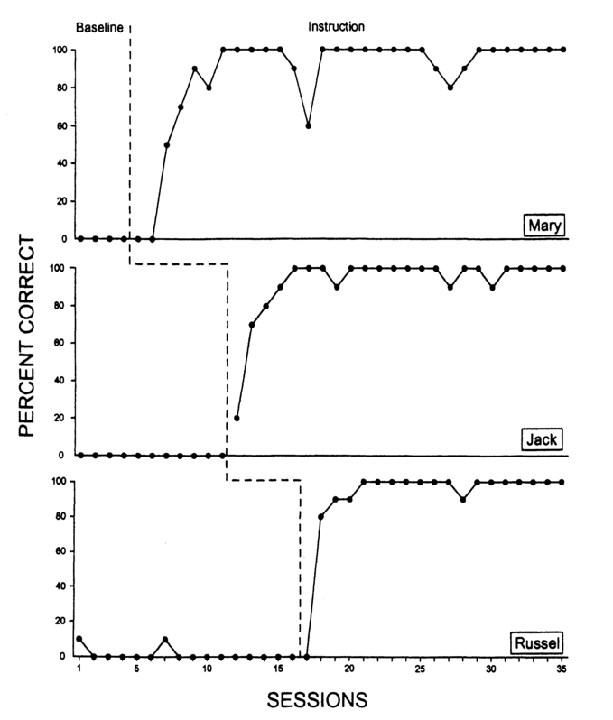
Figure 8.10 Percentage of correctly asking the question "What's that?" when pointing to a novel stimulus across baseline and instruction phases of a multiple baseline design for three students with autism (Taylor & Harris, 1995).
Jackson and Mathews (1995) used a multiple baseline design across settings (that is, various grocery stores) to examine the effectiveness of a public posting program on contributions to a senior citizens center. Grocery store customers were given the opportunity to redeem coupons or to donate the worth of the coupon to the senior center. The experimental condition consisted of posting signs around the store that included visual and written instructions and feedback on the value of coupons donated by customers the previous week in that particular store. Figure 8.11 demonstrates the effects of the public posting condition over baseline conditions across three stores. The percentage and value of coupons donated are plotted separately. The results of this public posting intervention are unclear. Baseline data did not achieve stability prior to the intervention in any of the three stores. As a result it would be difficult to predict what performance would be like if baseline assessment had continued and the intervention had not been implemented. Additionally, there are no clear level changes between baseline and intervention conditions across the three stores. These results seem to implicate that the intervention had little effect on shoppers behavior above and beyond baseline conditions. This study also demonstrates an interesting variation of the multiple baseline across settings design. There is no control exerted over the number or identity of the individuals who purchase items in each store during any given assessment period. This variation of a multiple baseline across settings design is frequently used in community behavior analysis applications (Greene, Winett, Van Houten, Geller, & Iwata, 1987).
In an example of a multiple baseline design across behaviors, Rasing and Duker (1992) examined the effects of a teaching protocol to train social skills to children with severe and profound hearing loss. The intervention was implemented across two classrooms (consisting of 4 and 5 children respectively). Experimental control was demonstrated using a multiple baseline design across social skills for each classroom. The teaching strategy consisted of modeling, role-play, corrective feedback for incorrect responding, and positive reinforcement for correct responding. The social skills taught included turn waiting during conversations, initiating interactions with others, and interacting with others. The mean percentage of intervals of appropriate and inappropriate instances of the target behaviors for each class was recorded during observation sessions. The results of the intervention for Class 2 are presented in Figure 8.12. These results indicate a reduction of inappropriate instances of all three target behaviors with the introduction of the intervention. The effects of the intervention for appropriate instances of the behaviors are less definitive. For turn waiting, the intervention produced a clear level change in responding for the class, however, differences between baseline and
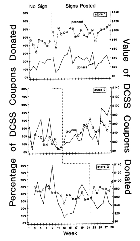
Figure 8.11 The effects of a public posting intervention across three stores on the percentage of coupons (designated by the open squares in the graphs) and value of coupons (designated by the closed dots in the graphs) per week that were donated to a local senior citizens center (Jackson & Mathews, 1995).
intervention for the other two target behaviors are less dramatic. Overall, the results of this intervention must be viewed with caution. Stable baselines were not established for appropriate instances of initiating interactions and interacting with others prior to introducing the intervention with the class. This violates one of the fundamental properties of single-case research design logic, as mentioned previously.
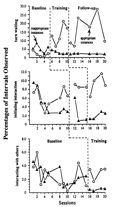
Figure 8.12 Percentage of intervals in which appropriate and inappropriate turn waiting, initiating interactions, and interacting with others was observed for a class of students with severe/profound hearing loss (Rasing & Duker, 1992).
This design demonstrates experimental control by sequentially applying the independent variable across multiple baselines (persons, behaviors, or settings). A confident interpretation of the effects of the independent variable can be obtained if there are visible changes in the data paths when and only when the independent variable is applied across the separate baselines. The multiple baseline design therefore does not require a withdrawal of treatment in order to demonstrate experimental control. This design option should be considered when it is expected that a withdrawal of treatment might not result in a return of behavior to previous baseline levels. Multiple baseline designs are often employed to examine the effectiveness of teaching strategies on the acquisition of skills as such skills are expected to maintain once instruction is withdrawn (Cuvo, 1979). The multiple baseline design would not be an appropriate option for behaviors that are in need of rapid elimination (such as behaviors that are dangerous to self or others) as measurement of responding prior to intervention is required.
The changing criterion design is used to increase or decrease the rate of responding of a behavior that is already in the repertoire of the individual. As the design has such a specific application it is seldom reported in the literature. This design demonstrates experimental control by showing that the target behavior achieves and stabilizes at a series of predetermined criteria of responding.
A baseline level of responding is initially established for the target behavior. Once behavior has stabilized under baseline conditions the experimenter establishes a criterion of responding that is more stringent than baseline levels of responding. The participant must achieve this criterion in order to access reinforcement. Once behavior stabilizes at this criterion an alternative criterion for responding is set and so on. The nature of the behavior must be of such that it requires multiple changes in criteria to be made before the desired rate of responding is achieved. There are no strict rules for calculating the magnitude of criterion change from one phase to the next. A general rule of thumb is that the criterion change should be small enough to be achievable but not so small that it will be exceeded. If responding exceeds or does not achieve the criterion level then experimental control is lost. Experimental control can also be enhanced if criteria are made less stringent from time to time during the intervention phase and the target behavior reverses to these criteria. A withdrawal design logic can therefore be incorporated within a changing criterion design without the need for the behavior to return to original baseline levels.
Bates, Renzaglia and Clees (1980) used a changing criterion design to examine the effectiveness of reinforcement contingencies to increase the work productivity of three adults with severe and profound developmental disabilities. One participant was taught to self-administer a penny following completion of two work units. The number of pennies needed to access a snack during break period were identified for the participant prior to each work period. The rate of work units per minute was measured for each work period. The criteria of work units per minute was systematically increased across fourteen phases during the intervention (i.e., the participant needed to earn more pennies in order to access a snack item). The results for this participant are illustrated in Figure 8.13. Overall, the patterns of participant responding stabilized around the criteria established by the experimenter. Interestingly, responding began to exceed the established criteria, particularly in the last three phases of the design. These data in the final phases of the design seem to indicate that a more stringent criterion for reinforcement should have been established at that point in order to regain experimental control.
The changing criterion design has a very specific application. The behaviors selected for change must already be in the repertoire of the individual. It must also be possible and appropriate to increase or decrease these behaviors in incremental steps. Cooper, Heron, and Heward (1987) note that this design is often mistakenly recommended for use when shaping new behaviors. A shaping program focuses on gradually changing the topography of behavior over time whereas the changing criterion design is suitable for examining changes in the level of responding of an already established behavior. It can be difficult to determine responding criteria for future phases of the design. If responding exceeds or does not reach the criterion within a phase then experimental control is lost for that phase of the design. In such instances it may be prudent to reverse the criterion to a level that had previously established stable responding. Experimental control can thus be re-established and a more sensitive criterion can be calculated for the following phase.
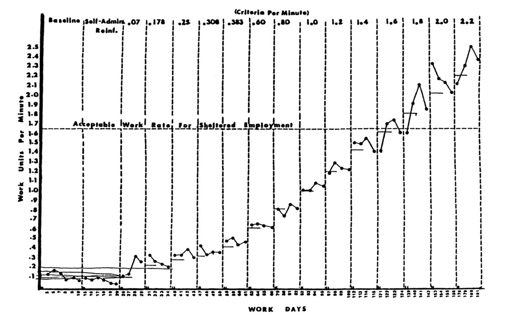
Figure 8.13 Use of a changing criterion design to systematically increase work units per minute for workers with developmenta disabilities (Bates, Renzaglia, & Clees, 1980).
The alternating treatment design is used to compare the effects of two or more contingencies or treatments on a target behavior. All treatment comparisons are implemented during a single phase of the design. Treatments are rapidly implemented in a random or semi-random order. Other potential extraneous variables such as time of day or therapist are held constant across the treatments in order to control their influence. Experimental control is demonstrated if there is a clear visible differentiation between treatments. If there is no clear difference between treatments it may be that each selected treatment is equally successful or that there is some extraneous factor influencing the results (e.g., carryover effects). Baseline levels of responding are sometimes assessed prior to the alternating treatment phase of the design. A prior baseline phase is not necessary in order to establish experimental control. On some occasions a baseline condition is implemented as part of the alternating treatments phase of the design in order to examine rate of responding without treatment. Alternating treatment designs are frequently used to assess the contingencies that maintain responding and to examine the comparative effectiveness of various treatment options.
Kennedy and Souza (1995) used an alternating treatment design to examine the contingencies that maintained severe eye poking for a young man with profound developmental disabilities. The duration of eye poking was measured across four conditions. Each condition was implemented during 10-minute sessions in a random order across days. In the no-attention condition the participant was seated at a table and received no social interactions. During the attention condition the therapist sat next to the participant and provided 10 seconds of social comments contingent on eye poking. During the demand condition the participant was taught to perform a domestic task. If the participant engaged in eye poking the task was removed for 15 seconds (negative reinforcement). In the recreation condition various magazines were provided and the participant was praised every 15 seconds in the absence of eye poking. The results of this analysis are presented in Figure 8.14. Eye poking only occurred during the no attention condition. The results of this intervention imply that eye poking served an automatic or self-stimulatory function for the participant.
In another example, Smith, Iwata, and Shore (1995) combined an alternating treatments design with a multiple baseline design to compare the effectiveness of participant-selected versus experimenter-selected reinforcers on the performance of four individuals with profound disabilities. A series of items were initially identified as reinforcing for the participants (e.g., mirror, light, music etc.). Participants were required to perform a free operant task (closing a microswitch or placing small blocks in a plastic bucket) during trials. Task performance under baseline conditions (in multiple baseline across participants format) was measured prior to the comparison phase of the design. In the experimenter selected reinforcer condition the therapist delivered a reinforcing item on a fixed-ratio (FR) 5 schedule. In the subject selected reinforcer condition the participant was allowed to choose from an array of reinforcing items on an FR 5 schedule. The experimenter and subject selected reinforcer conditions were compared in the alternating treatments phase of the design. The results of this experiment are shown in Figure 8.15. The results of the multiple baseline design show stable responding or decreasing trends prior to the reinforcement conditions. There is an increase in responding with the implementation of the reinforcement contingencies for the first three participants. Variability in responding under baseline conditions for participant 4 make data difficult to interpret for that participant. The results of the alternating treatments design phase demonstrates that there is little difference in responding across the two reinforcement conditions for all four participants.
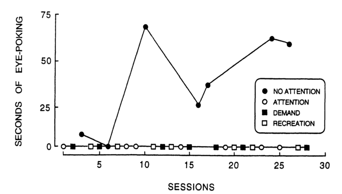
Figure 8.14 Total seconds of eye poking during four assessment conditions presented in an alternating treatments design (Kennedy & Souza, 1995).
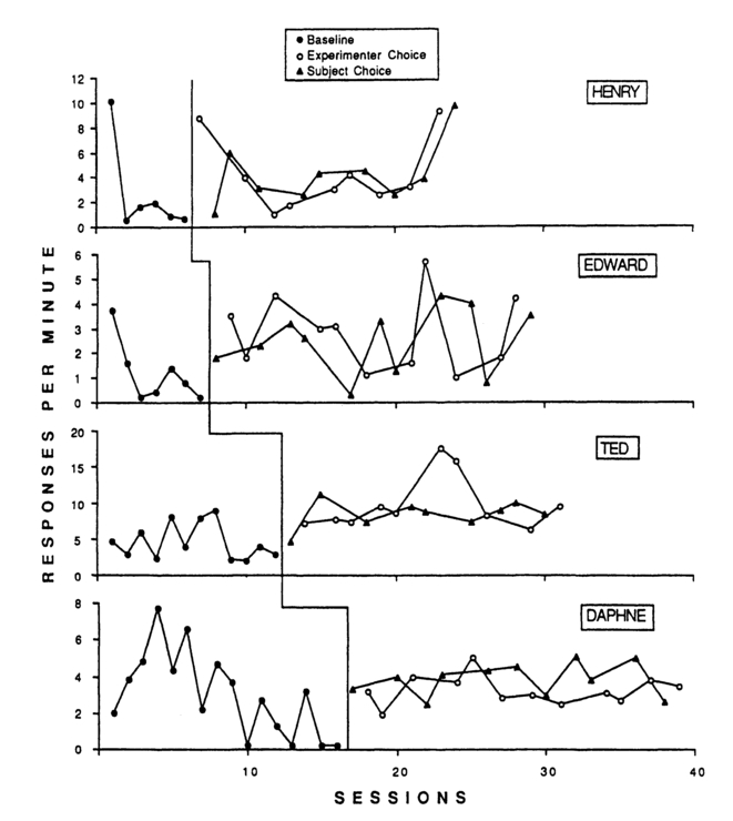
Figure 8.15 The effects of experimenter-selected versus subject-selected reinforcers on responses per minute for four individuals with developmental disabilities (Smith, Iwata, & Shore, 1995).
Alternating treatment designs allow for the comparative assessment of various treatments or contingencies within one experimental phase. It is therefore more efficient than reversal or multiple baseline designs for examining the effectiveness of one or more treatments as it does not require multiple phases or withdrawals of treatment. Additionally, the alternating treatment design does not require a baseline assessment prior to intervention nor a reversal to baseline levels during the evaluation of treatment. If responding under baseline is of interest to the therapist then a baseline condition can be included and assessed as a treatment within the alternating treatments phase of the design. This design can be a useful protocol for examining the comparative effectiveness of different treatments to reduce dangerous behaviors. The alternating treatment design produces relatively rapid results and does not invoke ethical concerns regarding extended baseline assessments for behaviors such as self-injury or aggression.
The experimental methods used by applied behavior analysts to evaluate the effects of interventions on target behaviors have been described in this chapter. These experimental designs can clarify the effects of the intervention by ruling out alternative explanations for changes in the target behavior. In other words, single-case experimental designs are used to identify the functional relationship between the intervention and the target behavior. Additionally, single-case designs can be used to examine the generalizability of interventions across persons, settings, and behaviors.
Single-case research designs typically use graphic display to present an ongoing visual presentation of the target behavior over time. The effectiveness of the intervention is evaluated by visually comparing the target behavior when the intervention is not available (baseline phase) and when it is applied (intervention phase). The target behavior should be fairly stable prior to implementing or removing the intervention. This allows for a clearer prediction of what the behavior would be like if these experimental conditions remained in place. It also allows for a clearer comparison between predicted and actual performance under the subsequent experimental phase. Variability or trends in data paths can temper any firm conclusions about the effectiveness of the intervention.
Several of the most frequently used design options were presented. The withdrawal or ABAB design consists of an A phase (baseline) and B phase (intervention) that are replicated. Experimental control is demonstrated if there is a visible difference in the data paths of the A and B phases and this difference is again demonstrated in the A and B phase replications. The multiple baseline design can examine the effects of an intervention across multiple persons, settings, or behaviors. The intervention is applied sequentially across multiple baselines, and experimental control is demonstrated if baseline responding changes at that point in time when the treatment variable is applied to each baseline. The changing criterion design is specifically used to examine incremental changes in the level of the target behavior over time. Experimental control is demonstrated if the level of responding matches the established criteria for responding during each phase of the design. Finally, the alternating treatments design is used to compare the effects of multiple interventions on the target behavior. Treatments are rapidly implemented in a random or semi-random order. Experimental control is demonstrated if there is a visible differentiation between treatments.
Selection of a research design is determined by the applied question of interest, constraints of the applied setting, nature of the target behavior and so on. The applied behavior analyst must find an appropriate balance between the need for experimental control and the constraints of the applied setting. For example, the ABAB design demonstrates the most powerful experimental control. However, this design may be difficult to implement in many instances for therapists or parents may be unwilling to withdraw or withhold treatments for extended periods of time. In such cases a multiple baseline design or alternating treatment design should be selected.