Chapter 7. Graphing Linear Equations and Inequalities in One and Two Variables
7.1. Objectives*
After completing the chapter, you should
Graphing Linear Equations and Inequalities In One Variable (Section 7.2)
understand the concept of a graph and the relationship between axes, coordinate systems, and dimension
be able to construct one-dimensional graphs
Plotting Points in the Plane (Section 7.3)
be familiar with the plane
know what is meant by the coordinates of a point
be able to plot points in the plane
Graphing Linear Equations in Two Variables (Section 7.8)
be able to relate solutions to a linear equation to lines
know the general form of a linear equation
be able to construct the graph of a line using the intercept method
be able to distinguish, by their equations, slanted, horizontal, and vertical lines
The Slope-Intercept Form of a Line (Section 7.5)
be more familiar with the general form of a line
be able to recognize the slope-intercept form of a line
be able to interpret the slope and intercept of a line
be able to use the slope formula to find the slope of a line
Graphing Equations in Slope-Intercept Form (Section 7.6)
be able to use the slope and intercept to construct the graph of a line
Finding the Equation of a Line (Section 7.7)
be able to find the equation of line using either the slope-intercept form or the point-slope form of a line
Graphing Linear Inequalities in Two Variables (Section 7.8)
be able to locate solutions linear inequalitites in two variables using graphical techniques
7.2. Graphing Linear Equations and Inequalities in One Variable *
Overview
Graphs
Axes, Coordinate Systems, and Dimension
Graphing in One Dimension
Graphs
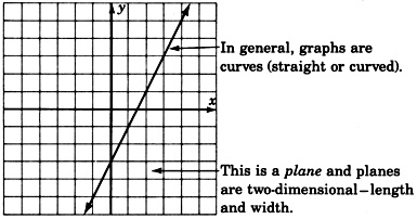
We have, thus far in our study of algebra, developed and used several methods for obtaining solutions to linear equations in both one and two variables. Quite often it is helpful to obtain a picture of the solutions to an equation. These pictures are called graphs and they can reveal information that may not be evident from the equation alone.
The geometric representation (picture) of the solutions to an equation is called the graph of the equation.
Axes, Coordinate Systems, and Dimension
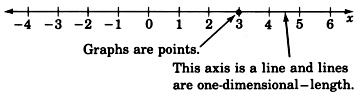
The basic structure of the graph is the axis. It is with respect to the axis that all solutions to an equation are located. The most fundamental type of axis is the number line.

We have the following general rules regarding axes.
| An equation in one variable requires one axis. |
| An equation in two variables requires two axes. |
| An equation in three variables requires three axes. |
| ... An equation in n variables requires n axes. |
We shall always draw an axis as a straight line, and if more than one axis is required, we shall draw them so they are all mutually perpendicular (the lines forming the axes will be at 90° angles to one another).
A system of axes constructed for graphing an equation is called a coordinate system.
The phrase graphing an equation is used frequently and should be interpreted as meaning geometrically locating the solutions to an equation.
We will not start actually graphing equations until Section Section 7.3, but in the following examples we will relate the number of variables in an equation to the number of axes in the coordinate system.
|
1. One-Dimensional Graphs:
If we wish to graph the equation 5x + 2 = 17 , we would need to construct a coordinate system consisting of a single axis (a single number line) since the equation consists of only one variable. We label the axis with the variable that appears in the equation. We might interpret an equation in one variable as giving information in one-dimensional space. Since we live in three-dimensional space, one-dimensional space might be hard to imagine. Objects in one-dimensional space would have only length, no width or depth. |
|
2. Two-Dimensional Graphs:
To graph an equation in two variables such as
y = 2x–3 , we would need to construct a coordinate system consisting of two mutually perpendicular number lines (axes). We call the intersection of the two axes the origin and label it with a 0. The two axes are simply number lines; one drawn horizontally, one drawn vertically. We might interpret equations in two variables as giving information in two-dimensional space. Objects in two-dimensional space would have length and width, but no depth. |
|
3. Three-Dimensional Graphs:
An equation in three variables, such as 3x
2 –4y
2 + 5z = 0 , requires three mutually perpendicular axes, one for each variable. We would construct the following coordinate system and graph. We might interpret equations in three variables as giving information about three-dimensional space. |
|
4. Four-Dimensional Graphs:
To graph an equation in four variables, such as 3x–2y + 8x–5w = –7 , would require four mutually perpendicular number lines. These graphs are left to the imagination. We might interpret equations in four variables as giving information in four-dimensional space. Four-dimensional objects would have length, width, depth, and some other dimension.
Black Holes These other spaces are hard for us to imagine, but the existence of “black holes” makes the possibility of other universes of one-, two-, four-, or n-dimensions not entirely unlikely. Although it may be difficult for us “3-D” people to travel around in another dimensional space, at least we could be pretty sure that our mathematics would still work (since it is not restricted to only three dimensions)! |

Graphing in One Dimension
Graphing a linear equation in one variable involves solving the equation, then locating the solution on the axis (number line), and marking a point at this location. We have observed that graphs may reveal information that may not be evident from the original equation. The graphs of linear equations in one variable do not yield much, if any, information, but they serve as a foundation to graphs of higher dimension (graphs of two variables and three variables).
Sample Set A
Example 7.1.
Graph the equation 3x–5 = 10 .
Solve the equation for x and construct an axis. Since there is only one variable, we need only one axis. Label the axis x .


Example 7.2.
Graph the equation 3x + 4 + 7x–1 + 8 = 31 .
Solving the equation we get,


Sample Set B
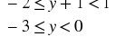
Example 7.3.
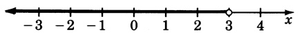
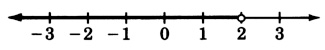
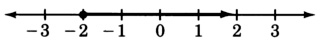
Graph the linear inequality  .
.
We proceed by solving the inequality.

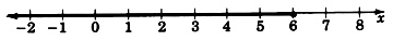
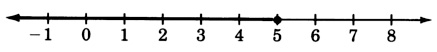
As we know, any value greater than or equal to 3 will satisfy the original inequality. Hence we have infinitely many solutions and, thus, infinitely many points to mark off on our graph. 
The closed circle at 3 means that 3 is included as a solution. All the points beginning at 3 and in the direction of the arrow are solutions.
Example 7.4.
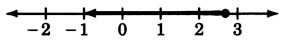
Graph the linear inequality –2y–1 > 3 .
We first solve the inequality.

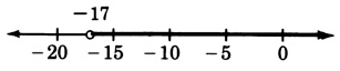
Thus, all numbers strictly less than − 2 will satisfy the inequality and are thus solutions.
Since − 2 itself is not to be included as a solution, we draw an open circle at − 2 . The solutions are to the left of − 2 so we draw an arrow pointing to the left of − 2 to denote the region of solutions.

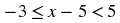
Example 7.5.
Graph the inequality  .
.
We recognize this inequality as a compound inequality and solve it by subtracting 1 from all three parts.
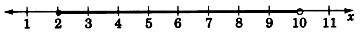
Thus, the solution is all numbers between − 3 and 0, more precisely, all numbers greater than or equal to − 3 but strictly less than 0.

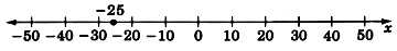
Example 7.6.
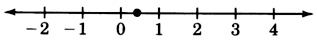
Graph the linear equation 5x = –125 .
The solution is x = –25 . Scaling the axis by units of 5 rather than 1, we obtain
Practice Set B

Exercises
For problems 1 - 25, graph the linear equations and inequalities.
Exercise 7.2.7.
8x − 1 = 7

Exercise 7.2.9.
x + 3 = 15
Exercise 7.2.11.
2x = 0
Exercise 7.2.13.


Exercise 7.2.15.

Exercise 7.2.17.
y − 5 < 3
Exercise 7.2.19.
z + 5 > 11
Exercise 7.2.21.
− 5t ≥ 10
Exercise 7.2.23.


Exercise 7.2.25.


Exercise 7.2.27.

Exercise 7.2.29.
6 ≤ x + 4 ≤ 7
Exercises for Review
Exercise 7.2.32. (Go to Solution)
(Section 4.2) List, if any should appear, the common factors in the expression 10x 4 − 15x 2 + 5x 6 .
Solutions to Exercises


7.3. Plotting Points in the Plane *
Overview
The Plane
Coordinates of a Point
Plotting Points
The Plane
We are now interested in studying graphs of linear equations in two variables. We know that solutions to equations in two variables consist of a pair of values, one value for each variable. We have called these pairs of values ordered pairs. Since we have a pair of values to graph, we must have a pair of axes (number lines) upon which the values can be located.
We draw the axes so they are perpendicular to each other and so that they intersect each other at their
0 ' s
. This point is called the origin.

These two lines form what is called a rectangular coordinate system. They also determine a plane.
x y-plane A plane is a flat surface, and a result from geometry states that through any two intersecting lines (the axes) exactly one plane (flat surface) may be passed. If we are dealing with a linear equation in the two variables x and y , we sometimes say we are graphing the equation using a rectangular coordinate system, or that we are graphing the equation in the x y-plane .
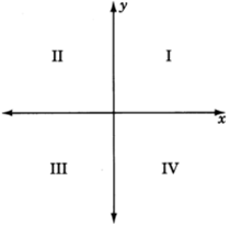
Notice that the two intersecting coordinate axes divide the plane into four equal regions. Since there are four regions, we call each one a quadrant and number them counterclockwise using Roman numerals. 
Recall that when we first studied the number line we observed the following:
For each real number there exists a unique point on the number line, and for each point on the number line we can associate a unique real number.
We have a similar situation for the plane.
For each ordered pair (a, b) , there exists a unique point in the plane, and to each point in the plane we can associate a unique ordered pair (a, b) of real numbers.
Coordinates of a Point
The numbers in an ordered pair that are associated with a particular point are called the coordinates of the point. The first number in the ordered pair expresses the point’s horizontal distance and direction (left or right) from the origin. The second number expresses the point’s vertical distance and direction (up or down) from the origin.
A positive number means a direction to the right or up. A negative
number means a direction to the left or down. 
Plotting Points
Since points and ordered pairs are so closely related, the two terms are sometimes used interchangeably. The following two phrases have the same meaning:
Plot the point (a, b) .
Plot the ordered pair (a, b) .
Both phrases mean: Locate, in the plane, the point associated with the ordered pair (a, b) and draw a mark at that position.
Sample Set A
Example 7.7.
Plot the ordered pair (2, 6) .
We begin at the origin. The first number in the ordered pair, 2, tells us we move 2 units to the right (
+ 2
means 2 units to the right) The second number in the ordered pair, 6, tells us we move 6 units up (
+ 6
means 6 units up). 
Practice Set A
Exercises
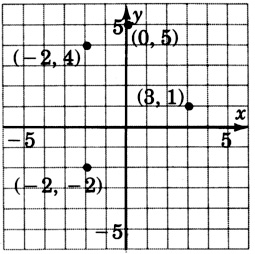
Exercise 7.3.2. (Go to Solution)
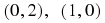
Plot the following ordered pairs. (Do not draw the arrows as in Practice Set A.) .
. 
Exercise 7.3.3.
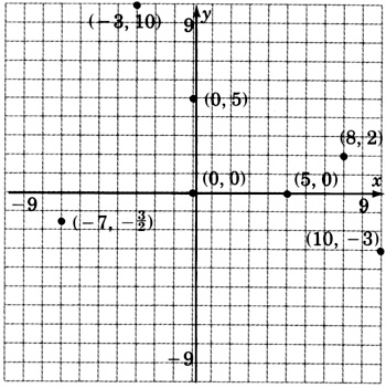
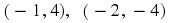
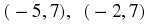
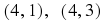
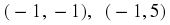
As accurately as possible, state the coordinates of the points that have been plotted on the following graph. 
Exercise 7.3.4. (Go to Solution)
Using ordered pair notation, what are the coordinates of the origin?
Exercise 7.3.5.
We know that solutions to linear equations in two variables can be expressed as ordered pairs. Hence, the solutions can be represented as points in the plane. Consider the linear equation y = 2x − 1 . Find at least ten solutions to this equation by choosing x-values between − 4 and 5 and computing the corresponding y-values . Plot these solutions on the coordinate system below. Fill in the table to help you keep track of the ordered pairs.
| x | ||||||||||||
| y |
 Keeping in mind that there are infinitely many ordered pair solutions to
y = 2x − 1
, speculate on the geometric structure of the graph of all the solutions. Complete the following statement:The name of the type of geometric structure of the graph of all the solutions to the linear equation
y = 2x − 1
seems to be __________ .Where does this figure cross the
y-axis
? Does this number appear in the equation
y = 2x − 1
?Place your pencil at any point on the figure (you may have to connect the dots to see the figure
clearly). Move your pencil exactly one unit to the right (horizontally). To get back onto the figure,
you must move your pencil either up or down a particular number of units. How many units must you move vertically to get back onto the figure, and do you see this number in the equation
y = 2x − 1
?
Keeping in mind that there are infinitely many ordered pair solutions to
y = 2x − 1
, speculate on the geometric structure of the graph of all the solutions. Complete the following statement:The name of the type of geometric structure of the graph of all the solutions to the linear equation
y = 2x − 1
seems to be __________ .Where does this figure cross the
y-axis
? Does this number appear in the equation
y = 2x − 1
?Place your pencil at any point on the figure (you may have to connect the dots to see the figure
clearly). Move your pencil exactly one unit to the right (horizontally). To get back onto the figure,
you must move your pencil either up or down a particular number of units. How many units must you move vertically to get back onto the figure, and do you see this number in the equation
y = 2x − 1
?
Exercise 7.3.6. (Go to Solution)
Consider the
x
y-plane
.  Complete the table by writing the appropriate inequalities.
| I | II | III | IV |
| x > 0 | x < 0 | x | x |
| y > 0 | y | y | y |
In the following problems, the graphs of points are called scatter diagrams and are frequently used by statisticians to determine if there is a relationship between the two variables under consideration. The first component of the ordered pair is called the input variable and the second component is called the output variable. Construct the scatter diagrams. Determine if there appears to be a relationship between the two variables under consideration by making the following observations: A relationship may exist if
as one variable increases, the other variable increases
as one variable increases, the other variable decreases
Exercise 7.3.7.
A psychologist, studying the effects of a placebo on assembly line workers at a particular industrial site, noted the time it took to assemble a certain item before the subject was given the placebo, x , and the time it took to assemble a similar item after the subject was given the placebo, y . The psychologist's data are
| x | y |
| 10 | 8 |
| 12 | 9 |
| 11 | 9 |
| 10 | 7 |
| 14 | 11 |
| 15 | 12 |
| 13 | 10 |

Exercise 7.3.8. (Go to Solution)
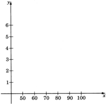
The following data were obtained in an engineer’s study of the relationship between the amount of pressure used to form a piece of machinery, x , and the number of defective pieces of machinery produced, y .
| x | y |
| 50 | 0 |
| 60 | 1 |
| 65 | 2 |
| 70 | 3 |
| 80 | 4 |
| 70 | 5 |
| 90 | 5 |
| 100 | 5 |
Exercise 7.3.9.
The following data represent the number of work days missed per year, x , by the employees of an insurance company and the number of minutes they arrive late from lunch, y .
| x | y |
| 1 | 3 |
| 6 | 4 |
| 2 | 2 |
| 2 | 3 |
| 3 | 1 |
| 1 | 4 |
| 4 | 4 |
| 6 | 3 |
| 5 | 2 |
| 6 | 1 |
Exercise 7.3.10. (Go to Solution)
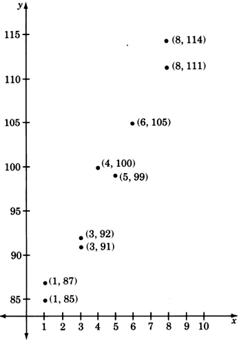
A manufacturer of dental equipment has the following data on the unit cost (in dollars), y , of a particular item and the number of units, x , manufactured for each order.
| x | y |
| 1 | 85 |
| 3 | 92 |
| 5 | 99 |
| 3 | 91 |
| 4 | 100 |
| 1 | 87 |
| 6 | 105 |
| 8 | 111 |
| 8 | 114 |

Exercises for Review

Exercise 7.3.12. (Go to Solution)
(Section 4.3) Supply the missing word. An __________ is a statement that two algebraic expressions are equal.
Exercise 7.3.13.
(Section 4.4) Simplify the expression 5x y(x y − 2x + 3y) − 2x y(3x y − 4x) − 15x y 2 .
Exercise 7.3.14. (Go to Solution)
(Section 5.2) Identify the equation x + 2 = x + 1 as an identity, a contradiction, or a conditional equation.
Exercise 7.3.15.
(Section 7.2) Supply the missing phrase. A system of axes constructed for graphing an equation is called a __________ .
Solutions to Exercises
Solution to Exercise 7.3.1. (Return to Exercise)
(Notice that the dotted lines on the graph are only for illustration and should not be included when plotting points.)

Solution to Exercise 7.3.6. (Return to Exercise)
| I | II | III | IV |
| x > 0 | x < 0 | x < 0 | x > 0 |
| y > 0 | y > 0 | y < 0 | y < 0 |

7.4. Graphing Linear Equations in Two Variables *
Overview
Solutions and Lines
General form of a Linear Equation
The Intercept Method of Graphing
Graphing Using any Two or More Points
Slanted, Horizontal, and Vertical Lines
Solutions and Lines
We know that solutions to linear equations in two variables can be expressed as ordered pairs. Hence, the solutions can be represented by point in the plane. We also know that the phrase “graph the equation” means to locate the solution to the given equation in the plane. Consider the equation y − 2x = − 3 . We’ll graph six solutions (ordered pairs) to this equation on the coordinates system below. We’ll find the solutions by choosing x-values (from − 1 to + 4 ), substituting them into the equation y − 2x = − 3 , and then solving to obtain the corresponding y-values . We can keep track of the ordered pairs by using a table.
y − 2x = − 3
| If x = | Then y = | Ordered Pairs |
| − 1 | − 5 | ( − 1, − 5 ) |
| 0 | − 3 | ( 0, − 3 ) |
| 1 | − 1 | ( 1, − 1 ) |
| 2 | 1 | ( 2, 1 ) |
| 3 | 3 | ( 3, 3 ) |
| 4 | 5 | ( 4, 5 ) |

We have plotted only six solutions to the equation y − 2x = − 3 . There are, as we know, infinitely many solutions. By observing the six points we have plotted, we can speculate as to the location of all the other points. The six points we plotted seem to lie on a straight line. This would lead us to believe that all the other points (solutions) also lie on that same line. Indeed, this is true. In fact, this is precisely why first-degree equations are called linear equations.


General Form of a Linear Equation
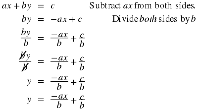
There is a standard form in which linear equations in two variables are written. Suppose that a , b , and c are any real numbers and that a and b cannot both be zero at the same time. Then, the linear equation in two variables
a x + b y = c
is said to be in general form.
We must stipulate that a and b cannot both equal zero at the same time, for if they were we would have
0x + 0y = c
0 = c
This statement is true only if c = 0 . If c were to be any other number, we would get a false statement.
Now, we have the following:
The graphing of all ordered pairs that solve a linear equation in two variables produces a straight line.
This implies,
The graph of a linear equation in two variables is a straight line.
From these statements we can conclude,
If an ordered pair is a solution to a linear equations in two variables, then it lies on the graph of the equation.
Also,
Any point (ordered pairs) that lies on the graph of a linear equation in two variables is a solution to that equation.
The Intercept Method of Graphing
When we want to graph a linear equation, it is certainly impractical to graph infinitely many points. Since a straight line is determined by only two points, we need only find two solutions to the equation (although a third point is helpful as a check).
When a linear equation in two variables is given in general from, a x + b y = c , often the two most convenient points (solutions) to fine are called the Intercepts: these are the points at which the line intercepts the coordinate axes. Of course, a horizontal or vertical line intercepts only one axis, so this method does not apply. Horizontal and vertical lines are easily recognized as they contain only one variable. (See Sample Set C .)

y-Intercept The point at which the line crosses the y-axis is called the y-intercept . The x-value at this point is zero (since the point is neither to the left nor right of the origin).
x-Intercept The point at which the line crosses the x-axis is called the x-intercept and the y-value at that point is zero. The y-intercept can be found by substituting the value 0 for x into the equation and solving for y . The x-intercept can be found by substituting the value 0 for y into the equation and solving for x .
Since we are graphing an equation by finding the intercepts, we call this method the intercept method
Sample Set A
Graph the following equations using the intercept method.
Example 7.8.
y − 2x = − 3
To find the y-intercept , let x = 0 and y = b .
Thus, we have the point ( 0, − 3 ) . So, if x = 0 , y = b = − 3 .
To find the x-intercept , let y = 0 and x = a .
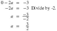
Thus, we have the point  . So, if
  ,
y = 0 .
,
y = 0 .
Construct a coordinate system, plot these two points, and draw a line through them. Keep in mind that every point on this line is a solution to the equation y − 2x = − 3 .
Example 7.9.
− 2x + 3y = 3
To find the y-intercept , let x = 0 and y = b .

Thus, we have the point ( 0, 1 ) . So, if x = 0 , y = b = 1 .
To find the x-intercept , let y = 0 and x = a .

Thus, we have the point  . So, if
 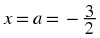 ,
y = 0 .
,
y = 0 .
Construct a coordinate system, plot these two points, and draw a line through them. Keep in mind that all the solutions to the equation − 2x + 3y = 3 are precisely on this line.

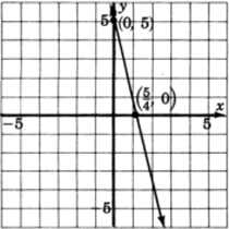
Example 7.10.
4x + y = 5
To find the y-intercept , let x = 0 and y = b .

Thus, we have the point ( 0, 5 ) . So, if x = 0 , y = b = 5 .
To find the x-intercept , let y = 0 and x = a .

Thus, we have the point  . So, if
  ,
y = 0 .
,
y = 0 .
Construct a coordinate system, plot these two points, and draw a line through them.
Graphing Using any Two or More Points
The graphs we have constructed so far have been done by finding two particular points, the intercepts. Actually, any two points will do. We chose to use the intercepts because they are usually the easiest to work with. In the next example, we will graph two equations using points other than the intercepts. We’ll use three points, the extra point serving as a check.
Sample Set B
Example 7.11.
x − 3y = − 10 .We can find three points by choosing three x-values and computing to find the corresponding y-values . We’ll put our results in a table for ease of reading.
Since we are going to choose x-values and then compute to find the corresponding y-values , it will be to our advantage to solve the given equation for y .

| x | y | ( x, y ) |
| 1 | If
x = 1 , then 
|

|
| − 3 | If
x = − 3 , then 
|

|
| 3 | If
x = 3 , then 
|

|
Thus, we have the three ordered pairs (points),  ,
,  ,
,  . If we wish, we can change the improper fractions to mixed numbers,
  ,
,  ,
,  .
.

Example 7.12.
4x + 4y = 0
We solve for y .

| x | y | ( x, y ) |
| 0 | 0 | ( 0, 0 ) |
| 2 | − 2 | ( 2, − 2 ) |
| − 3 | 3 | ( − 3, 3 ) |

Notice that the x − and y-intercepts are the same point. Thus the intercept method does not provide enough information to construct this graph.
When an equation is given in the general form a x + b y = c , usually the most efficient approach to constructing the graph is to use the intercept method, when it works.
Practice Set B
Graph the following equations.
Slanted, Horizontal, and Vertical Lines
In all the graphs we have observed so far, the lines have been slanted. This will always be the case when both variables appear in the equation. If only one variable appears in the equation, then the line will be either vertical or horizontal. To see why, let’s consider a specific case:
Using the general form of a line, a x + b y = c , we can produce an equation with exactly one variable by choosing a = 0 , b = 5 , and c = 15 . The equation a x + b y = c then becomes
0x + 5y = 15
Since 0⋅( any number ) = 0 , the term 0x is 0 for any number that is chosen for x .
Thus,
0x + 5y = 15
becomes
0 + 5y = 15
But, 0 is the additive identity and 0 + 5y = 5y .
5y = 15
Then, solving for y we get
y = 3
This is an equation in which exactly one variable appears.
This means that regardless of which number we choose for x , the corresponding y-value is 3. Since the y-value is always the same as we move from left-to-right through the x-values , the height of the line above the x-axis is always the same (in this case, 3 units). This type of line must be horizontal.
An argument similar to the one above will show that if the only variable that appears is x , we can expect to get a vertical line.
Sample Set C
Example 7.13.
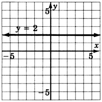
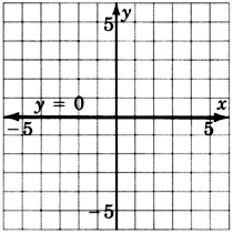
Graph y = 4 .The only variable appearing is y . Regardless of which x-value we choose, the y-value is always 4. All points with a y-value of 4 satisfy the equation. Thus we get a horizontal line 4 unit above the x-axis .
| x | y | ( x, y ) |
| − 3 | 4 | ( − 3, 4 ) |
| − 2 | 4 | ( − 2, 4 ) |
| − 1 | 4 | ( − 1, 4 ) |
| 0 | 4 | ( 0, 4 ) |
| 1 | 4 | ( 1, 4 ) |
| 2 | 4 | ( 2, 4 ) |
| 3 | 4 | ( 3, 4 ) |
| 4 | 4 | ( 4, 4 ) |

Example 7.14.
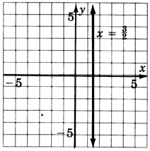
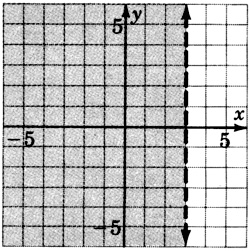
Graph x = − 2 .The only variable that appears is x . Regardless of which y-value we choose, the x-value will always be − 2 . Thus, we get a vertical line two units to the left of the y-axis .
| x | y | ( x,y ) |
| − 2 | − 4 | ( − 2, − 4 ) |
| − 2 | − 3 | ( − 2, − 3 ) |
| − 2 | − 2 | ( − 2, − 2 ) |
| − 2 | − 1 | ( − 2, − 1 ) |
| − 2 | 0 | ( − 2, 0 ) |
| − 2 | 1 | ( − 2, 1 ) |
| − 2 | 2 | ( − 2, 0 ) |
| − 2 | 3 | ( − 2, 3 ) |
| − 2 | 4 | ( − 2, 4 ) |
 |
Practice Set C
Summarizing our results we can make the following observations:
When a linear equation in two variables is written in the form a x + b y = c , we say it is written in general form.
To graph an equation in general form it is sometimes convenient to use the intercept method.
A linear equation in which both variables appear will graph as a slanted line.
A linear equation in which only one variable appears will graph as either a vertical or horizontal line. x = a graphs as a vertical line passing through a on the x-axis . y = b graphs as a horizontal line passing through b on the y-axis .
Exercises
For the following problems, graph the equations.
Exercise 7.4.8.
3x − 2y = 6

Exercise 7.4.10.
x − 3y = 5
Exercise 7.4.12.
2x + 5y = 10
Exercise 7.4.14.
− 2x + 3y = − 12
Exercise 7.4.16.
4y − x − 12 = 0
Exercise 7.4.18.
− 2x + 5y = 0
Exercise 7.4.20.
0x + y = 3
Exercise 7.4.22.

Exercise 7.4.24.

Exercise 7.4.26.
y = 3
Exercise 7.4.28.
− 4y = 20
Exercise 7.4.30.
− 3x = − 9
Exercise 7.4.32.
Construct the graph of all the points that have coordinates ( a, a ) , that is, for each point, the
x − and
y-values are the same.
 Calculator Problems
Exercise 7.4.34.
1.96x + 2.05y = 6.55
Exercise 7.4.36.
626.01x − 506.73y = 2443.50
Exercises for Review
Exercise 7.4.37. (Go to Solution)
(Section 2.3) Name the property of real numbers that makes 4 + x = x + 4 a true statement.
Exercise 7.4.38.
(Section 3.3) Supply the missing word. The absolute value of a number a , denoted | a | , is the __________ from a to 0 on the number line.
Exercise 7.4.41. (Go to Solution)
(Section 7.3) Supply the missing word. The coordinate axes divide the plane into four equal regions called __________.
Solutions to Exercises


7.5. The Slope-Intercept Form of a Line*
Overview
The General Form of a Line
The Slope-Intercept Form of a Line
Slope and Intercept
The Formula for the Slope of a Line
The General Form of a Line
We have seen that the general form of a linear equation in two variables is a x + b y = c (Section Section 7.4). When this equation is solved for y , the resulting form is called the slope-intercept form. Let's generate this new form.
This equation is of the form
y = m
x + b
if we replace  with
m
and constant
with
m
and constant  with
b
. (Note: The fact that we let
with
b
. (Note: The fact that we let  is unfortunate and occurs beacuse of the letters we have chosen to use in the general form. The letter
b
occurs on both sides of the equal sign and may not represent the same value at all. This problem is one of the historical convention and, fortunately, does not occur very often.)
is unfortunate and occurs beacuse of the letters we have chosen to use in the general form. The letter
b
occurs on both sides of the equal sign and may not represent the same value at all. This problem is one of the historical convention and, fortunately, does not occur very often.)
The following examples illustrate this procedure.
Example 7.15.
Solve 3x + 2y = 6 for y .

This equation is of the form
y = m
x + b
. In this case,  and
b = 3
.
and
b = 3
.
Example 7.16.
Solve – 15x + 5y = 20 for y .
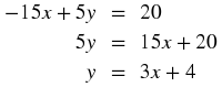
This equation is of the form y = m x + b . In this case, m = 3 and b = 4 .
Example 7.17.
Solve 4x – y = 0 for y .

This equation is of the form y = m x + b . In this case, m = 4 and b = 0 . Notice that we can write y = 4x as y = 4x + 0 .
The Slope-Intercept Form of a Line
A linear equation in two variables written in the form y = m x + b is said to be in slope-intercept form.
Sample Set A
The following equations are in slope-intercept form:
Example 7.18.

Example 7.19.

Example 7.20.

Example 7.21.

The following equations are not in slope-intercept form:
Example 7.22.

Example 7.23.

Example 7.24.

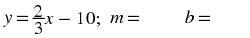
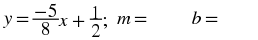
Practice Set A
The following equation are in slope-intercept form. In each case, specify the slope and y-intercept .


Slope and Intercept
When the equation of a line is written in slope-intercept form, two important properties of the line can be seen: the slope and the intercept. Let's look at these two properties by graphing several lines and observing them carefully.
Sample Set B
Example 7.25.
Graph the line y = x − 3 .
| x | y | ( x, y ) |
| 0 | − 3 | (0, − 3) |
| 4 | 1 | (4, 1) |
| − 2 | − 5 | ( − 2, − 5) |

Looking carefully at this line, answer the following two questions.
Problem 1.
At what number does this line cross the y-axis ? Do you see this number in the equation?
Solution
The line crosses the y-axis at – 3 .
Problem 2.
Place your pencil at any point on the line. Move your pencil exactly one unit horizontally to the right. Now, how many units straight up or down must you move your pencil to get back on the line? Do you see this number in the equation?
Solution
After moving horizontally one unit to the right, we must move exactly one vertical unit up. This number is the coefficient of x .
Example 7.26.
Graph the line  .
.
| x | y | ( x, y ) |
| 0 | 1 | (0, 1) |
| 3 | 3 | (3, 3) |
| − 3 | − 1 | ( − 3, − 1) |

Looking carefully at this line, answer the following two questions.
Problem 1.
At what number does this line cross the y-axis ? Do you see this number in the equation?
Solution
The line crosses the y-axis at + 1 .
Problem 2.
Place your pencil at any point on the line. Move your pencil exactly one unit horizontally to the right. Now, how many units straight up or down must you move your pencil to get back on the line? Do you see this number in the equation?
Solution
After moving horizontally one unit to the right, we must move exactly  unit upward. This number is the coefficient of
x
.
unit upward. This number is the coefficient of
x
.
Practice Set B
Example 7.27.
Graph the line y = − 3x + 4 .
| x | y | (x, y) |
| 0 | ||
| 3 | ||
| 2 |

Looking carefully at this line, answer the following two questions.
Exercise 7.5.7. (Go to Solution)
At what number does the line cross the y-axis ? Do you see this number in the equation?
Exercise 7.5.8. (Go to Solution)
Place your pencil at any point on the line. Move your pencil exactly one unit horizontally to the right. Now, how many units straight up or down must you move your pencil to get back on the line? Do you see this number in the equation?
In the graphs constructed in Sample Set B and Practice Set B, each equation had the form y = m x + b . We can answer the same questions by using this form of the equation (shown in the diagram).
y -Intercept
Exercise 7.5.9.
At what number does the line cross the y-axis ? Do you see this number in the equation?
Solution
In each case, the line crosses the y-axis at the constant b . The number b is the number at which the line crosses the y-axis , and it is called the y-intercept . The ordered pair corresponding to the y-intercept is (0, b).
Exercise 7.5.10.
Place your pencil at any point on the line. Move your pencil exactly one unit horizontally to the right. Now, how many units straight up or down must you move your pencil to get back on the line? Do you see this number in the equation?
Solution
To get back on the line, we must move our pencil exactly m vertical units.
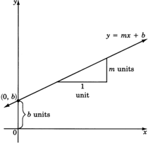
The number m is the coefficient of the variable x . The number m is called the slope of the line and it is the number of units that y changes when x is increased by 1 unit. Thus, if x changes by 1 unit, y changes by m units. Since the equation y = m x + b contains both the slope of the line and the y-intercept , we call the form y = m x + b the slope-intercept form.
The slope-intercept form of a straight line is y = m x + b The slope of the line is m , and the y-intercept is the point (0 , b) .
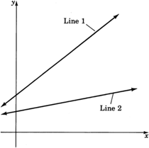
The word slope is really quite appropriate. It gives us a measure of the steepness of the line. Consider two lines, one with slope  and the other with slope 3. The line with slope 3 is steeper than is the line with slope
  . Imagine your pencil being placed at any point on the lines. We make a 1-unit increase in the
x
-value by moving the pencil one unit to the right. To get back to one line we need only move vertically
. Imagine your pencil being placed at any point on the lines. We make a 1-unit increase in the
x
-value by moving the pencil one unit to the right. To get back to one line we need only move vertically  unit, whereas to get back onto the other line we need to move vertically 3 units.

Sample Set C
Find the slope and the y -intercept of the following lines.
Example 7.28.
y = 2x + 7. The line is in the slope-intercept form y = m x + b. The slope is m , the coefficient of x . Therefore, m = 2. The y-intercept is the point (0, b). Since b = 7 , the y-intercept is (0, 7).

Example 7.29.
y = − 4x + 1. The line is in slope-intercept form y = m x + b. The slope is m , the coefficient of x . So, m = − 4. The y-intercept is the point (0, b). Since b = 1 , the y-intercept is (0, 1).

Example 7.30.
3x + 2y = 5. The equation is written in general form. We can put the equation in slope-intercept form by solving for y .
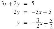
Now the equation is in slope-intercept form.

Practice Set C
The Formula for the Slope of a Line
We have observed that the slope is a measure of the steepness of a line. We wish to develop a formula for measuring this steepness.
It seems reasonable to develop a slope formula that produces the following results:
Steepness of line 1 > steepness of line 2.
Consider a line on which we select any two points. We’ll denote these points with the ordered pairs (x 1, y 1 ) and (x 2, y 2 ) . The subscripts help us to identify the points.
(x 1, y 1 ) is the first point. Subscript 1 indicates the first point. (x 2, y 2 ) is the second point. Subscript 2 indicates the second point.

The difference in x values (x 2 − x 1 ) gives us the horizontal change, and the difference in y values (y 2 − y 1 ) gives us the vertical change. If the line is very steep, then when going from the first point to the second point, we would expect a large vertical change compared to the horizontal change. If the line is not very steep, then when going from the first point to the second point, we would expect a small vertical change compared to the horizontal change.


We are comparing changes. We see that we are comparing

This is a comparison and is therefore a ratio. Ratios can be expressed as fractions. Thus, a measure of the steepness of a line can be expressed as a ratio.
The slope of a line is defined as the ratio
Mathematically, we can write these changes as 
The slope of a nonvertical line passing through the points (x
1,
y
1 ) and (x
2,
y
2 ) is found by the formula
Sample Set D
For the two given points, find the slope of the line that passes through them.
Example 7.31.
( 0, 1 ) and ( 1, 3 ) .Looking left to right on the line we can choose (x
1,
y
1 ) to be ( 0, 1 ) , and (x
2,
y
2 ) to be ( 1, 3 ) . Then,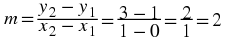
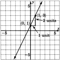 This line has slope 2. It appears fairly steep. When the slope is written in fraction form,
  , we can see, by recalling the slope formula, that as
x
changes 1 unit to the right (because of the + 1 )
y
changes 2 units upward (because of the + 2 ).
, we can see, by recalling the slope formula, that as
x
changes 1 unit to the right (because of the + 1 )
y
changes 2 units upward (because of the + 2 ).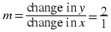 Notice that as we look left to right, the line rises.
Example 7.32.
(2, 2 ) and (4, 3 ) .Looking left to right on the line we can choose (x
1,
y
1 ) to be (2, 2 ) and (x
2,
y
2 ) to be (4, 3 ). Then,
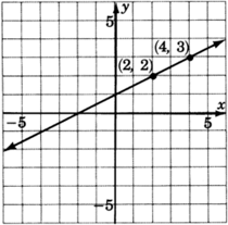 This line has slope
  . Thus, as
x
changes 2 units to the right (because of the + 2 ),
y
changes 1 unit upward (because of the + 1 ).
. Thus, as
x
changes 2 units to the right (because of the + 2 ),
y
changes 1 unit upward (because of the + 1 ). Notice that in examples 1 and 2, both lines have positive slopes, + 2 and
  , and both lines rise as we look left to right.
Example 7.33.
( − 2, 4) and (1, 1) .Looking left to right on the line we can choose (x
1,
y
1 ) to be ( − 2, 4) and (x
2,
y
2 ) to be (1, 1) . Then,
 This line has slope − 1. When the slope is written in fraction form,
  , we can see that as
x
changes 1 unit to the right (because of the + 1 ),
y
changes 1 unit downward (because of the − 1 ).Notice also that this line has a negative slope and declines as we look left to right.
, we can see that as
x
changes 1 unit to the right (because of the + 1 ),
y
changes 1 unit downward (because of the − 1 ).Notice also that this line has a negative slope and declines as we look left to right.
Example 7.34.
( 1, 3 ) and ( 5, 3 ) .
 This line has 0 slope. This means it has no rise and, therefore, is a horizontal line. This does not mean that the line has no slope, however.
Example 7.35.
( 4, 4 ) and ( 4, 0 ) .This problem shows why the slope formula is valid only for nonvertical lines. 
 Since division by 0 is undefined, we say that vertical lines have undefined slope. Since there is no real number to represent the slope of this line, we sometimes say that vertical lines have undefined slope, or no slope.
Practice Set D
Exercise 7.5.12. (Go to Solution)
Find the slope of the line passing through ( 2, 1 ) and ( 6, 3 ) . Graph this line on the graph of problem 2 below.
Exercise 7.5.13. (Go to Solution)
Find the slope of the line passing through (3, 4 ) and (5, 5 ) . Graph this line. 
Exercise 7.5.14. (Go to Solution)
Compare the lines of the following problems. Do the lines appear to cross? What is it called when lines do not meet (parallel or intersecting)? Compare their slopes. Make a statement about the condition of these lines and their slopes.
Before trying some problems, let’s summarize what we have observed.
Exercise 7.5.15.
The equation y = m x + b is called the slope-intercept form of the equation of a line. The number m is the slope of the line and the point (0, b ) is the y-intercept .
Exercise 7.5.16.
The slope, m, of a line is defined as the steepness of the line, and it is the number of units that y changes when x changes 1 unit.
Exercise 7.5.17.
The formula for finding the slope of a line through any two given points (x
1 ,y
1 ) and (x
2 ,y
2 ) is 
Exercise 7.5.18.
The fraction  represents the
Exercise 7.5.19.
As we look at a graph from left to right, lines with positive slope rise and lines with negative slope decline.
Exercise 7.5.20.
Parallel lines have the same slope.
Exercise 7.5.21.
Horizontal lines have 0 slope.
Exercise 7.5.22.
Vertical lines have undefined slope (or no slope).
Exercises
For the following problems, determine the slope and y-intercept of the lines.
Exercise 7.5.24.
y = 2x + 9
Exercise 7.5.26.
y = 7x + 10
Exercise 7.5.28.
y = − 2x + 8
Exercise 7.5.30.
y = − x − 6
Exercise 7.5.32.
2y = 4x + 8
Exercise 7.5.34.
− 5y = 15x + 55
Exercise 7.5.36.


Exercise 7.5.38.


Exercise 7.5.40.
− 3y = 5x + 8
Exercise 7.5.42.
− y = x + 1
Exercise 7.5.44.
3x − y = 7
Exercise 7.5.46.
− 6x − 7y = − 12
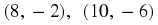
For the following problems, find the slope of the line through the pairs of points.
Exercise 7.5.48.
(1, 6), (4,9)
Exercise 7.5.50.
(3, 5), (4,7)
Exercise 7.5.52.
(0, 5), (2,-6)
Exercise 7.5.54.
(3, -9), (5,1)
Exercise 7.5.56.
(-5, 4), (-1,0)
Exercise 7.5.58.
(9, 12), (6,0)
Exercise 7.5.60.
(-2, -6), (-4,-1)
Exercise 7.5.62.
(-6, -6), (-5,-4)
Exercise 7.5.64.
(-4, -2), (0,0)
Exercise 7.5.66.
(4, -2), (4,7)
Exercise 7.5.68.
(4, 2), (6,2)
Exercise 7.5.70.
Do lines with a positive slope rise or decline as we look left to right?
Exercise 7.5.71. (Go to Solution)
Do lines with a negative slope rise or decline as we look left to right?
Exercise 7.5.72.
Make a statement about the slopes of parallel lines.
 Calculator Problems
For the following problems, determine the slope and y-intercept of the lines. Round to two decimal places.
Exercise 7.5.74.
8.09x + 5.57y = − 1.42
Exercise 7.5.76.
− 6.003x − 92.388y = 0.008
For the following problems, find the slope of the line through the pairs of points. Round to two decimal places.
Exercise 7.5.78.
(33.1, 8.9), (42.7, − 1.06)
Exercise 7.5.80.
(0.00426, − 0.00404), ( − 0.00191, − 0.00404)
Exercise 7.5.82.
( − 0.0000567, − 0.0000567), ( − 0.00765, 0.00764)
Exercises for Review
Exercise 7.5.85. (Go to Solution)
(Section 5.6) When four times a number is divided by five, and that result is decreased by eight, the result is zero. What is the original number?

Solutions to Exercises


Solution to Exercise 7.5.7. (Return to Exercise)
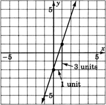
The line crosses the y-axis at + 4 . After moving horizontally 1 unit to the right, we must move exactly 3 units downward.


Solution to Exercise 7.5.14. (Return to Exercise)
The lines appear to be parallel. Parallel lines have the same slope, and lines that have the same slope are parallel. 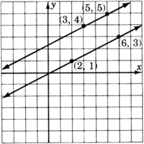


7.6. Graphing Equations in Slope-Intercept Form *
Overview
Using the Slope and Intercept to Graph a Line
Using the Slope and Intercept to Graph a Line
When a linear equation is given in the general form, a x + b y = c , we observed that an efficient graphical approach was the intercept method. We let x = 0 and computed the corresponding value of y , then let y = 0 and computed the corresponding value of x .
When an equation is written in the slope-intercept form, y = m x + b , there are also efficient ways of constructing the graph. One way, but less efficient, is to choose two or three x-values and compute to find the corresponding y-values . However, computations are tedious, time consuming, and can lead to errors. Another way, the method listed below, makes use of the slope and the y-intercept for graphing the line. It is quick, simple, and involves no computations.
Graphing Method
Plot the y-intercept (0, b) .
Determine another point by using the slope m .
Draw a line through the two points.
Recall that we defined the slope m
as the ratio  . The numerator
y
2 − y
1
represents the number of units that
y
changes and the denominator
x
2 − x
1
represents the number of units that
x
changes. Suppose
. The numerator
y
2 − y
1
represents the number of units that
y
changes and the denominator
x
2 − x
1
represents the number of units that
x
changes. Suppose  . Then
p
is the number of units that
y
changes and
q
is the number of units that
x
changes. Since these changes occur simultaneously, start with your pencil at the
y-intercept , move
p
units in the appropriate vertical direction, and then move
q
units in the appropriate horizontal direction. Mark a point at this location.
. Then
p
is the number of units that
y
changes and
q
is the number of units that
x
changes. Since these changes occur simultaneously, start with your pencil at the
y-intercept , move
p
units in the appropriate vertical direction, and then move
q
units in the appropriate horizontal direction. Mark a point at this location.
Sample Set A
Graph the following lines.
Example 7.36.

The y-intercept is the point ( 0, 2 ) . Thus the line crosses the y-axis 2 units above the origin. Mark a point at ( 0, 2 ) .

The slope, m , is
 . This means that if we start at any point on the line and move our pencil 3 units up and then 4 units to the right, we’ll be back on the line. Start at a known point, the
y-intercept ( 0, 2 ) . Move up 3 units, then move 4 units to the right. Mark a point at this location. (Note also that
. This means that if we start at any point on the line and move our pencil 3 units up and then 4 units to the right, we’ll be back on the line. Start at a known point, the
y-intercept ( 0, 2 ) . Move up 3 units, then move 4 units to the right. Mark a point at this location. (Note also that  . This means that if we start at any point on the line and move our pencil 3 units down and 4 units to the left, we’ll be back on the line. Note also that
  . This means that if we start at any point on the line and move to the right 1 unit, we’ll have to move up 3 / 4 unit to get back on the line.)
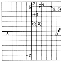
Draw a line through both points.
Example 7.37.
The y-intercept is the point
 . Thus the line crosses the
y-axis
. Thus the line crosses the
y-axis
 above the origin. Mark a point at
  , or
, or  .
.
The slope, m , is
 . We can write
  as
as  . Thus, we start at a known point, the
y-intercept
. Thus, we start at a known point, the
y-intercept
 , move down one unit (because of the − 1 ), then move right 2 units. Mark a point at this location.
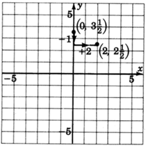
Draw a line through both points.

Example 7.38.

We can put this equation into explicit slope-intercept by writing it as
 .The
y-intercept is the point ( 0, 0 ) , the origin. This line goes right through the origin.
.The
y-intercept is the point ( 0, 0 ) , the origin. This line goes right through the origin.
The slope, m , is
 . Starting at the origin, we move up 2 units, then move to the right 5 units. Mark a point at this location.
Draw a line through the two points.
Example 7.39.
y = 2x − 4
The y-intercept is the point ( 0, − 4 ) . Thus the line crosses the y-axis 4 units below the origin. Mark a point at ( 0, − 4 ) .
The slope, m , is 2. If we write the slope as a fraction,
 , we can read how to make the changes. Start at the known point ( 0, − 4 ) , move up 2 units, then move right 1 unit. Mark a point at this location.
Draw a line through the two points.
Practice Set A
Use the y-intercept and the slope to graph each line.

Excercises
For the following problems, graph the equations.

Exercise 7.6.4.

Exercise 7.6.6.

Exercise 7.6.8.

Exercise 7.6.10.
Exercise 7.6.12.
y = − 2x + 1
Exercise 7.6.14.


Exercise 7.6.16.
y = x
Exercise 7.6.18.
3y − 2x = − 3
Exercise 7.6.20.
x + y = 0
Excersise for Review

Exercise 7.6.25. (Go to Solution)
(Section 7.5) Find the slope of the line passing through the points ( − 1, 5) and (2, 3) .
Solutions to Exercises


7.7. Finding the Equation of a Line *
Overview
The Slope-Intercept and Point-Slope Forms
The Slope-Intercept and Point-Slope Forms
In the pervious sections we have been given an equation and have constructed the line to which it corresponds. Now, however, suppose we're given some geometric information about the line and we wish to construct the corresponding equation. We wish to find the equation of a line.
We know that the formula for the slope of a line is  We can find the equation of a line using the slope formula in either of two ways:
Example 7.40.
If we’re given the slope, m , and any point (x, y 1 ) on the line, we can substitute this information into the formula for slope.Let (x, y 1 ) be the known point on the line and let (x,y) be any other point on the line. Then

Since this equation was derived using a point and the slope of a line, it is called the point-slope form of a line.
Example 7.41.
If we are given the slope, m , y-intercept, (0,b) , we can substitute this information into the formula for slope.Let (0,b) be the y-intercept and (x,y) be any other point on the line. Then,

Since this equation was derived using the slope and the intercept, it was called the slope-intercept form of a line.
We summarize these two derivations as follows.
We can find the equation of a line if we’re given either of the following sets of information:
- The slope,
m, and the
y-intercept, (0,b), by substituting these values into
This is the slope-intercept form.
- The slope,
m, and any point, (x
1 ,y
1 ), by substituting these values into
This is the point-slope form.
Notice that both forms rely on knowing the slope. If we are given two points on the line we may still find the equation of the line passing through them by first finding the slope of the line, then using the point-slope form.
It is customary to use either the slope-intercept form or the general form for the final form of the line. We will use the slope-intercept form as the final form.
Sample Set A
Find the equation of the line using the given information.
Example 7.42.
m = 6 ,y-intercept (0,4)
Since we’re given the slope and the y-intercept, we’ll use the slope-intercept form. m = 6,b = 4.

Example 7.43.
Since we’re given the slope and the
y-intercept, we’ll use the slope-intercept form. 
Example 7.44.
 Write the equation in slope-intercept form.
Since we’re given the slope and some point, we’ll use the point-slope form.

Example 7.45.
 Write the equation in slope-intercept form.
Since we’re given the slope and some point, we’ll use the point-slope form.

Example 7.46.
 Write the equation in slope-intercept form.
We’re given the slope and a point, but careful observation reveals that this point is actually the y-intercept. Thus, we’ll use the slope-intercept form. If we had not seen that this point was the y-intercept we would have proceeded with the point-slope form. This would create slightly more work, but still give the same result.

Example 7.47.
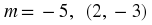
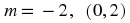
The two points (4,1) and (3,5). Write the equation in slope-intercept form.
Since we’re given two points, we’ll find the slope first.

Now, we have the slope and two points. We can use either point and the point-slope form.
| Using (4, 1) | Using (3, 5) |
|
|
We can see that the use of either point gives the same result.
Practice Set A
Find the equation of each line given the following information. Use the slope-intercept form as the final form of the equation.
Sample Set B
Example 7.48.
Find the equation of the line passing through the point (4, – 7) having slope 0.
We’re given the slope and some point, so we’ll use the point-slope form. With m = 0 and (x 1 ,y 1 ) as (4, – 7), we have

This is a horizontal line.
Example 7.49.
Find the equation of the line passing through the point (1,3) given that the line is vertical.
Since the line is vertical, the slope does not exist. Thus, we cannot use either the slope-intercept form or the point-slope form. We must recall what we know about vertical lines. The equation of this line is simply x = 1.
Practice Set B
Exercise 7.7.11. (Go to Solution)
Find the equation of the line passing through the point ( – 2,9) having slope 0.
Exercise 7.7.12. (Go to Solution)
Find the equation of the line passing through the point ( – 1,6) given that the line is vertical.
Sample Set C
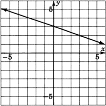
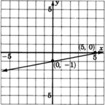
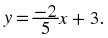
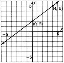
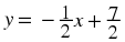
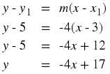
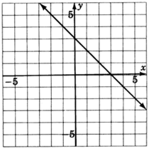
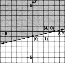
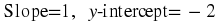
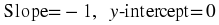
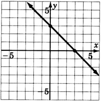
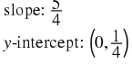
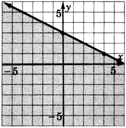
Example 7.50.
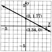
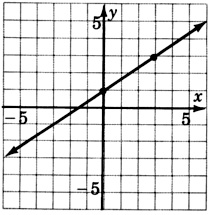
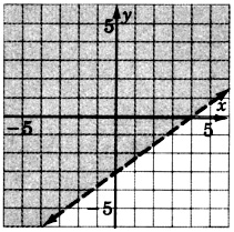
Reading only from the graph, determine the equation of the line.
The slope of the line is  and the line crosses the
y-axis at the point (0, – 3). Using the slope-intercept form we get
and the line crosses the
y-axis at the point (0, – 3). Using the slope-intercept form we get

Practice Set C

Exercises
For the following problems, write the equation of the line using the given information in slope-intercept form.
Exercise 7.7.15.
m = 2, y-intercept (0,5)
Exercise 7.7.17.
m = 5, y-intercept (0, – 3)
Exercise 7.7.19.
m = – 4, y-intercept (0,0)

Exercise 7.7.21.
m = 3, (1,4)
Exercise 7.7.23.
m = 2, (1,4)
Exercise 7.7.25.
m = – 3, (3,0)
Exercise 7.7.27.
m = – 6, (0,0)
Exercise 7.7.29.
(0,0), (3,2)
Exercise 7.7.31.
(4,1), (6,3)
Exercise 7.7.33.
(5, – 3), (6,2)
Exercise 7.7.35.
( – 1,5), (4,5)
Exercise 7.7.37.
(2,7), (2,8)
Exercise 7.7.39.
(0,0), (1,1)
Exercise 7.7.41.
(1,6), ( – 1, – 6)
Exercise 7.7.43.
(0, – 4), (5,0)
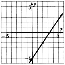
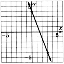
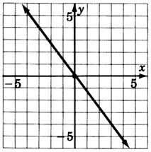
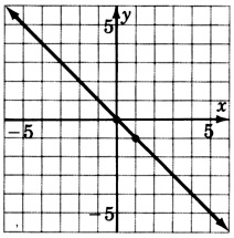
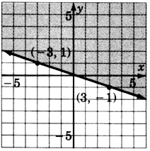
For the following problems, read only from the graph and determine the equation of the lines.
Exercise 7.7.45.


Exercise 7.7.47.

Exercise 7.7.49.
Exercises for Review

Exercise 7.7.52. (Go to Solution)
(Section 7.4) Supply the missing word. The point at which a line crosses the y-axis is called the __________.
Exercise 7.7.53.
(Section 7.5) Supply the missing word. The __________ of a line is a measure of the steepness of the line.
Exercise 7.7.54. (Go to Solution)
(Section 7.5) Find the slope of the line that passes through the points (4,0) and ( – 2, – 6).

Solutions to Exercises


7.8. Graphing Linear Inequalities in Two Variables *
Overview
Location of Solutions
Method of Graphing
Location of Solutions
In our study of linear equations in two variables, we observed that all the solutions to the equation, and only the solutions to the equation, were located on the graph of the equation. We now wish to determine the location of the solutions to linear inequalities in two variables. Linear inequalities in two variables are inequalities of the forms:

A straight line drawn through the plane divides the plane into two half-planes.
The straight line is called the boundary line.

Recall that when working with linear equations in two variables, we observed that ordered pairs that produced true statements when substituted into an equation were called solutions to that equation. We can make a similar statement for inequalities in two variables. We say that an inequality in two variables has a solution when a pair of values has been found such that when these values are substituted into the inequality a true statement results.
As with equations, solutions to linear inequalities have particular locations in the plane. All solutions to a linear inequality in two variables are located in one and only in one entire half-plane. For example, consider the inequality
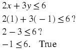
2x + 3y ≤ 6

All the solutions to the inequality 2x + 3y ≤ 6 lie in the shaded half-plane.
Example 7.51.
Point A(1, − 1) is a solution since
Example 7.52.
Point B(2, 5) is not a solution since

Method of Graphing
The method of graphing linear inequalities in two variables is as follows:
Graph the boundary line (consider the inequality as an equation, that is, replace the inequality sign with an equal sign).
If the inequality is ≤ or ≥ , draw the boundary line solid. This means that points on the line are solutions and are part of the graph.
If the inequality is < or > , draw the boundary line dotted. This means that points on the line are not solutions and are not part of the graph.
Determine which half-plane to shade by choosing a test point.
If, when substituted, the test point yields a true statement, shade the half-plane containing it.
If, when substituted, the test point yields a false statement, shade the half-plane on the opposite side of the boundary line.
Sample Set A
Example 7.53.
Graph 3x − 2y ≥ − 4 .
1. Graph the boundary line. The inequality is ≥ so we’ll draw the line solid. Consider the inequality as an equation. 3x − 2y = − 4
| x | y | ( x, y ) |

|

|

|

2. Choose a test point. The easiest one is ( 0, 0 ) . Substitute ( 0, 0 ) into the original inequality.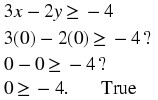 Shade the half-plane containing ( 0, 0 ) .
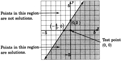
Example 7.54.
Graph x + y − 3 < 0 .
1. Graph the boundary line:
x + y − 3 = 0 . The inequality is < so we’ll draw the line dotted. 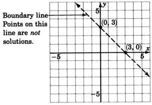
2. Choose a test point, say (0, 0) . Shade the half-plane containing (0, 0) .
Example 7.55.
Graph y ≤ 2x .
Graph the boundary line y = 2x . The inequality is ≤ , so we’ll draw the line solid.

- Choose a test point, say ( 0, 0 ) .
Shade the half-plane containing ( 0, 0 ) . We can’t! ( 0, 0 ) is right on the line! Pick another test point, say ( 1, 6 ) .
Shade the half-plane on the opposite side of the boundary line.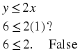

Example 7.56.
Graph y > 2 .
1. Graph the boundary line
y = 2 . The inequality is > so we’ll draw the line dotted. 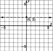
2. We don’t really need a test point. Where is
y > 2 ?
Above the line
y = 2! Any point above the line clearly has a
y-coordinate greater than 2. 
Practice Set A
Solve the following inequalities by graphing.
Exercises
Solve the inequalities by graphing.
Exercise 7.8.6.
x + y ≤ 1
Exercise 7.8.8.
− x + 5y − 10 < 0
Exercise 7.8.10.
2x + 5y − 15 ≥ 0
Exercise 7.8.12.
x ≥ 2
Exercise 7.8.14.
x − y < 0
Exercise 7.8.16.
− 2x + 4y > 0
Exercises for Review

Exercise 7.8.18.
(Section 7.2) Supply the missing word. The geometric representation (picture) of the solutions to an equation is called the __________ of the equation.

Exercise 7.8.21. (Go to Solution)
(Section 7.7) Write the equation of the line that has slope 4 and passes through the point ( − 1, 2 ) .
Solutions to Exercises


7.9. Summary of Key Concepts *
Summary of Key Concepts
The geometric representation (picture) of the solutions to an equation is called the graph of the equation.
An axis is the most basic structure of a graph. In mathematics, the number line is used as an axis.
A system of axes that is constructed for graphing an equation is called a coordinate system.
The phrase graphing an equation is interpreted as meaning geometrically locating the solutions to that equation.
A graph may reveal information that may not be evident from the equation.
A rectangular coordinate system is constructed by placing two number lines at 90 ° angles. These lines form a plane that is referred to as the xy -plane.
For each ordered pair ( a,b ), there exists a unique point in the plane, and for each point in the plane we can associate a unique ordered pair ( a,b ) of real numbers.
When graphed, a linear equation produces a straight line.
The general form of a linear equation in two variables is a x + b y = c, where a and b are not both 0.
The graphing of all ordered pairs that solve a linear equation in two variables produces a straight line.The graph of a linear equation in two variables is a straight line.If an ordered pair is a solution to a linear equation in two variables, then it lies on the graph of the equation.Any point (ordered pair) that lies on the graph of a linear equation in two variables is a solution to that equation.
An intercept is a point where a line intercepts a coordinate axis.
The intercept method is a method of graphing a linear equation in two variables by finding the intercepts, that is, by finding the points where the line crosses the x-axis and the y-axis .
An equation in which both variables appear will graph as a slanted line.A linear equation in which only one variable appears will graph as either a vertical or horizontal line. x = a graphs as a vertical line passing through a on the x-axis . y = b graphs as a horizontal line passing through b on the y-axis .
The slope of a line is a measure of the line’s steepness. If
(x
1
,y
1
)
and
(x
2
,y
2
)
are any two points on a line, the slope of the line passing through these points can be found using the slope formula.
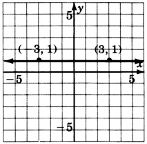
Moving left to right, lines with positive slope rise, and lines with negative slope decline.
An equation written in slope intercept form can be graphed by
Plotting the y-intercept ( 0,b ) .
Determining another point using the slope, m .
Drawing a line through these two points.

A straight line drawn through the plane divides the plane into two half-planes. The straight line is called a boundary line.
A solution to an inequality in two variables is a pair of values that produce a true statement when substituted into the inequality.
All solutions to a linear inequality in two variables are located in one, and only one, half-plane.
7.10. Exercise Supplement *
Exercise Supplement
Graphing Linear Equations and Inequalities in One Variable (Section 7.2)
For the following problems, graph the equations and inequalities.
Exercise 7.10.2.
4x − 3 = − 7

Exercise 7.10.4.
10x − 16 < 4

Exercise 7.10.6.


Exercise 7.10.8.
− 16 ≤ 5x − 1 ≤ − 11
Exercise 7.10.10.

Plotting Points in the Plane (Section 7.3)

Exercise 7.10.12.
As accurately as possible, state the coordinates of the points that have been plotted on the graph. 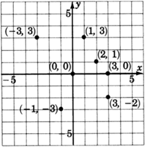
Graphing Linear Equations in Two Variables (Section 7.4)
Exercise 7.10.13. (Go to Solution)
What is the geometric structure of the graph of all the solutions to the linear equation y = 4x − 9 ?
Graphing Linear Equations in Two Variables (Section 7.4) - Graphing Equations in Slope-Intercept Form (Section 7.6)
For the following problems, graph the equations.
Exercise 7.10.14.
y − x = 2
Exercise 7.10.16.
− 2x + 3y = − 6
Exercise 7.10.18.
4(x − y) = 12
Exercise 7.10.20.
y = − 3
Exercise 7.10.22.
x = 4
Exercise 7.10.24.
x = 0
The Slope-Intercept Form of a Line (Section 7.5)
Exercise 7.10.26.
Write the slope-intercept form of a straight line.
Exercise 7.10.27. (Go to Solution)
The slope of a straight line is a __________ of the steepness of the line.
Exercise 7.10.28.
Write the formula for the slope of a line that passes through the points (x 1 ,y) and (x 2 ,y) .
For the following problems, determine the slope and y-intercept of the lines.
Exercise 7.10.30.
y = 3x − 11
Exercise 7.10.32.
y = − x + 2
Exercise 7.10.34.
y = x
Exercise 7.10.36.
3y = 4x + 9
Exercise 7.10.38.
2y = 9x
Exercise 7.10.40.
7y + 3x = 10
Exercise 7.10.42.
5y − 10x − 15 = 0
Exercise 7.10.44.
7y + 2x = 0
For the following problems, find the slope, if it exists, of the line through the given pairs of points.
Exercise 7.10.46.

Exercise 7.10.48.

Exercise 7.10.50.

Exercise 7.10.52.


Exercise 7.10.54.

Exercise 7.10.56.
Moving left to right, lines with __________ slope rise while lines with __________ slope decline.
Finding the Equation of a Line (Section 7.7)
For the following problems, write the equation of the line using the given information. Write the equation in slope-intercept form.
Exercise 7.10.58.

Exercise 7.10.60.
Exercise 7.10.62.


Exercise 7.10.64.

Exercise 7.10.66.


Exercise 7.10.68.

Exercise 7.10.70.

Exercise 7.10.72.


Exercise 7.10.74.
Exercise 7.10.76.
Exercise 7.10.78.

Exercise 7.10.80.

Exercise 7.10.82.
Exercise 7.10.84.

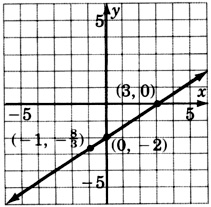
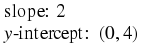
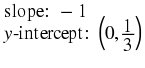
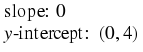
For the following problems, reading only from the graph, determine the equation of the line.
Exercise 7.10.86.


Exercise 7.10.88.


Exercise 7.10.90.


Graphing Linear Inequalities in Two Variables (Section 7.8)
For the following problems, graph the inequalities.
Exercise 7.10.92.
y ≤ x + 2

Exercise 7.10.94.

Exercise 7.10.96.
2x + 5y ≥ 20
Exercise 7.10.98.
y ≥ − 2
Exercise 7.10.100.
y ≤ 0
Solutions to Exercises


7.11. Proficiency Exam *
Proficiency Exam
For the following problems, construct a coordinate system and graph the inequality.
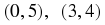
Exercise 7.11.3. (Go to Solution)
(Section 7.2) Plot the ordered pairs
(3, 1),( − 2, 4),(0, 5),( − 2, − 2)
. 
Exercise 7.11.4. (Go to Solution)
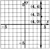
(Section 7.3) As accurately as possible, label the coordinates of the points that have been plotted on the graph. 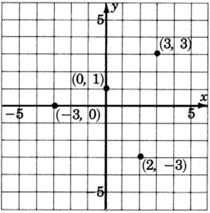
Exercise 7.11.5. (Go to Solution)
(Section 7.4) What is the geometric structure of the graph of all the solutions to the equation 2y + 3x = − 4 ?
Exercise 7.11.6. (Go to Solution)
(Section 7.4) In what form is the linear equation in two variables a x + b y = c ?
Exercise 7.11.7. (Go to Solution)
(Section 7.5) In what form is the linear equation in two variables y = m x + b ?
Exercise 7.11.8. (Go to Solution)
(Section 7.4) If an ordered pair is a solution to a linear equation in two variables, where does it lie geometrically?
Exercise 7.11.9. (Go to Solution)
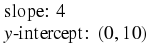
(Section 7.5) Consider the graph of  . If we were to place our pencil at any point on the line and then move it horizontally
7 units
to the right, how many units and in what direction would we have to move our pencil to get back on the line?
. If we were to place our pencil at any point on the line and then move it horizontally
7 units
to the right, how many units and in what direction would we have to move our pencil to get back on the line?
For the following two problems, find the slope, if it exists, of the line containing the following points.
Exercise 7.11.12. (Go to Solution)
(Section 7.5) Determine the slope and y − intercept of the line 3y + 2x + 1 = 0 .
Exercise 7.11.13. (Go to Solution)
(Section 7.5) As we look at a graph left to right, do lines with a positive slope rise or decline?
For the following problems, find the equation of the line using the information provided. Write the equation in slope-intercept form.


For the following problems, graph the equation of inequality.


Exercise 7.11.25. (Go to Solution)
(Section 7.7) Reading only from the graph, determine the equation of the line.