CHAPTER 6

Unsupervised Learning

UNSUPERVISED LEARNING includes a host of exploratory techniques that can be used to gain insight into data, often when there is no outcome variable or clear target. Although around for over a century, principal components analysis remains a data science staple and it is introduced along with MultivariateStats.jl. Probabilistic principal components analysis (PPCA) is considered next and an expectation-maximization algorithm for PPCA is implemented in Julia this is the first of two examples in this chapter that illustrate Julia as a base language for data science. Clustering, or unsupervised classification, is introduced along with the famous k-means clustering technique and Clustering.jl. A mixture of probabilistic principal components analyzers is then discussed and implemented, thereby providing the second example of Julia as a base language for data science.

6.1  INTRODUCTION

Unsupervised learning differs from supervised learning (Chapter 5) in that there are no labelled observations. It may be that there are labels but none are known a priori, it may be that some labels are known but the data are being treated as if unlabelled, or it may be the case that there are no labels per se. Because there are no labelled observations, it might be advantageous to lean towards statistical approaches and models — as opposed to machine learning — when tackling unsupervised learning problems. In a statistical framework, we can express our uncertainty in mathematical terms, and use clearly defined models and procedures with well-understood assumptions. Statistical approaches have many practical advantages, e.g., we may be able to write down likelihoods and compare models using likelihood-based criteria.

Suppose n realizations x₁, …, x_n of p-dimensional random variables X₁, …, X_n are observed, where X_i = (X_i1, X_i2, …, X_ip)′ for i = 1, …, n. As mentioned in Section 3.1, the quantity $\mathcal{X}$ = (X₁, X₂, …, X_n)’ can be considered a random matrix and its realization is called a data matrix. Recall also that a matrix A with all entries constant is called a constant matrix. Now, each X_i is a p × 1 random vector and, for our present purposes, it will be helpful to consider some results for random vectors. Let X and Y be p × 1 random vectors. Then,

$\mathbb{E}\left[X+Y\right]=\mathbb{E}\left[X\right]+\mathbb{E}\left[Y\right],$

and, if A, B, and C are m × n, p × q, and m × q constant matrices, respectively, then

$\mathbb{E}\left[AXB+C\right]=A\mathbb{E}\left[X\right]B+C.$

Suppose X has mean μ. Then, the covariance matrix of X is

$\sum =\mathbb{V}\text{ar}\left[X\right]=\mathbb{E}\left[\left(X-\mu \right){\left(X-\mu \right)}^{\prime }\right].$

Suppose p-dimensional X has mean μ and q-dimensional Y has mean θ. Then,

$\text{Cov}\left[X,Y\right]=\mathbb{E}\left[\left(X-\mu \right){\left(Y-\theta \right)}^{\prime }\right].$

The covariance matrix Σ of p-dimensional X can be written

$\Sigma =\left(\begin{array}{cccc}{\sigma }_{11}& {\sigma }_{12}& \cdots & {\sigma }_{1p}\\ {\sigma }_{21}& {\sigma }_{22}& \cdots & {\sigma }_{2p}\\ ⋮& ⋮& \ddots & ⋮\\ {\sigma }_{p1}& {\sigma }_{p2}& \cdots & {\sigma }_{pp}\end{array}\right).$

The elements σ_ii are variances and σ_ij, where i ≠ j, are the co-variances. The matrix Σ is symmetric because σ_ij = σ_ji. Also, Σ is positive semi-definite, i.e., for any p × 1 constant vector a = (a₁, …, a_p)’,

$\text{a}\prime \Sigma \text{a\hspace{0.17em}}\ge 0\text{.}$

Suppose C is a q × p constant matrix and c is a q × 1 constant vector. Then, the covariance matrix of Y = CX + c is

$\mathbb{V}\text{ar}\left[Y\right]=C\Sigma C^{\prime }.$

In general, the covariance matrix Σ is positive semi-definite. Therefore, the eigenvalues of Σ are non-negative, and are denoted

${\kappa }_1\ge {\kappa }_2\ge \cdots \ge {\kappa }_p\ge 0.$

Eigenvalues are also known as characteristic roots. Write v_i to denote the eigenvector corresponding to the eigenvalue κ_i, for i = 1, …, p. Eigenvectors are also known as characteristic vectors. Without loss of generality, it can be assumed that the eigenvectors are orthonormal, i.e.,

${v^{\prime }}_i{v}_i=1$

and

${v^{\prime }}_i{v}_j=0$

for i ≠ j. The eigenvalues and eigenvectors satisfy

$\Sigma v_i={\kappa }_i{v}_i,$

(6.1)

for i = 1, …, p.

Write V = v₁, …, v_p) and

$K=\text{diag}\left\{{\kappa }_1,\dots ,{\kappa }_p\right\}=\left(\begin{array}{cccc}{\kappa }_1& 0& \cdots & 0\\ 0& {\kappa }_2& \cdots & 0\\ ⋮& ⋮& \ddots & ⋮\\ 0& 0& \cdots & {\kappa }_p\end{array}\right).$

Then, (6.1) can be written

$\Sigma V=VK.$

Note that V′V = I_p, and

$\Sigma =VK{V}^{\prime }=V{K}^{1/2}{V}^{\prime }V{K}^{1/2}{V}^{\prime },$

where

$K^{1/2}=\text{diag}\left\{\sqrt{{\kappa }_1},\dots ,\sqrt{{\kappa }_p}\right\}.$

The determinant of the covariance matrix Σ can be written

$\begin{array}{l}|\Sigma |=\left|VK{V}^{\prime }\right|=\left|K\right|\\ ={\kappa }_1\times {\kappa }_2\times \cdots \times {\kappa }_p={\displaystyle \prod _{i=1}^p{\kappa }_i}.\end{array}$

The total variance of the covariance matrix Σ can be written

$\text{tr}\{\Sigma \}=\text{tr}\left\{K\right\}={\kappa }_1+{\kappa }_2+\cdots +{\kappa }_p.$

The determinant and total variance are sometimes used as summaries of the total scatter amongst the p variables. Note that some background on eigenvalues is provided in Appendix C.1.

6.2  PRINCIPAL COMPONENTS ANALYSIS

In general, observed data will contain correlated variables. The objective of principal components analysis is to replace the observed variables by a number of uncorrelated variables that explain a sufficiently large amount of the variance in the data. Before going into mathematical details, it will be helpful to understand the practical meaning of a principal component. The first principal component is the direction of most variation in the data. The second principal component is the direction of most variation in the data conditional on it being orthogonal to the first principal component. In general, for r ∈ (1, p], the rth principal component is the direction of most variation in the data conditional on it being orthogonal to the first r − 1 principal components. There are several mathematical approaches to motivating principal components analysis and the approach followed here is based on that used by Fujikoshi et al. (2010).

Let X be a p-dimensional random vector with mean μ and co-variance matrix Σ. Let κ₁ ≥ κ₂ ≥ … ≥ κ_ρ ≥ 0 be the (ordered) eigenvalues of Σ, and let v₁, v₂, …, v_p be the corresponding eigenvectors. The ith principal component of X is

$W_i={{\mathbf{v}}^{\prime }}_i\left(\mathbf{X}-\mathit{\mu }\right),$

(6.2)

for i = 1, …, p. Which we can write as

$W=V^{\prime }\left(X-\mathit{\mu }\right),$

(6.3)

where W = (W₁, …, W_p) and V = (v₁, … v_p).

Now, it is helpful to consider some properties of W. First of all, because $\mathbb{E}\left[X\right]=\mu$,

$\mathbb{E}\left[W\right]=0.$

Recalling that $\mathbb{V}\text{ar}\left[\mathbf{X}\right]$ = Σ = VKV′, we have

$\begin{array}{l}\mathbb{V}\text{ar}\left[\mathbf{W}\right]=V^{\prime }\mathbb{V}\text{ar}\left[X\right]V\\ =V^{\prime }\left(VK{V}^{\prime }\right)V\\ =\left(V^{\prime }V\right)K\left(V^{\prime }V\right)=K.\end{array}$

(6.4)

Rearranging (6.3),

$V^{\prime }X=V^{\prime }\mathit{\mu }+W,$

and left-multiplying by V gives

$X=\mu +VX=\mathit{\mu }+{\displaystyle \sum _{i=1}^p{v}_i{W}_i}.$

From (6.4), we can develop the result that

$\begin{array}{r}{\displaystyle \sum _{i=1}^p\mathbb{V}\text{ar}}\left[W_i\right]=\text{tr}\left\{K\right\}=\text{tr}\left\{K{V}^{\prime }V\right\}\\ =\text{tr}\left\{VK{V}^{\prime }\right\}=\text{tr}\left\{\Sigma \right\}.\end{array}$

Now, the proportion of the total variation explained by the jth principal component is

$\frac{{\kappa }_i}{\text{tr}\left\{K\right\}}=\frac{{\kappa }_i}{\text{tr}\left\{\Sigma \right\}}.$

Therefore, the proportion of the total variation explained by the first k principal components is

$\frac{{\sum }_{i=1}^k{\kappa }_i}{\text{tr}\left\{\Sigma \right\}}.$

To understand how the theoretical explanation of a principal component relates to the intuition given at the beginning of this section, consider

$W=v^{\prime }\left(X-\mu \right)$

such that v′v = 1. Now,

$\mathbb{V}\text{ar}\left[W\right]=v^{\prime }\Sigma v$

and we can write

$v=a_1{v}_1+\cdots +a_p{v}_p=Va$

for a′a = 1. Therefore,

$\mathbb{V}\text{ar}\left[W\right]=a_1^2{\kappa }_1+\cdots +a_p^2{\kappa }_p.$

(6.5)

Now, maximizing (6.5) subject to the constraint a′a = 1 gives $\mathbb{V}\text{ar}\left[W\right]$ = κ₁, i.e., a₁ = 1 and a_j = 0 for j > 1. In other words, $\mathbb{V}\text{ar}\left[W\right]$ is maximized at W = W₁, i.e., the first principal component.

Now suppose that W is uncorrelated with the first r − 1 < p principal components W₁, …, W_r−1. We have

$\text{Cov}\left[W,W_i\right]=\mathbb{E}\left[v^{\prime }\left(X-\mathit{\mu }\right){\left(X-\mathit{\mu }\right)}^{\prime }{v}_i\right]={\kappa }_i{c}_i$

and so c_i = 0 for i = 1, …, r − 1. Maximizing (6.5) subject to the constraint c_i = 0, for i = 1, …, r − 1, gives $\mathbb{V}\text{ar}\left[W\right]$ = κ_r. In other words, $\mathbb{V}\text{ar}\left[W\right]$ is maximized at W = Wr, i.e., the rth principal component.

Illustrative Example: Crabs Data

The following code block performs principal components analyses on the crabs data.

using LinearAlgebra

## function to do pca via SVD

  function pca_svd(X)

  n,p = size(X)

  k = min(n,p)

  S = svd(X)

  D = S.S[1:k]

  V = transpose(S.Vt)[:,1:k]

  sD = /(D, sqrt(n-1))

  rotation = V

  projection = *(X, V)

  return(Dict(

   "sd" => sD,

   "rotation" => rotation,

   "projection" => projection

  ))

end

## crab_mat_c is a Float array with 5 continuous mearures

## each variable is mean centered

crab_mat = convert(Array{Float64}, df_crabs[[:FL, :RW, :CL, :CW, : BD]])

mean_crab = mean(crab_mat, dims = 1)

crab_mat_c = crab_mat .- mean_crab

pca1 = pca_svd(crab_mat)

## df for plotting

## label is the combination of sp and sex

pca_df2 = DataFrame(

 pc1 = pca1["projection"][:,1],

 pc2 = pca1["projection"][:,2],

 pc3 = pca1["projection"][:,3],

 pc4 = pca1["projection"][:,4],

 pc5 = pca1["projection"][:,5],

 label = map(string, repeat(1:4, inner = 50))

)

More than 98% of the variation in the data is explained by the first principal component, with subsequent principal components accounting for relatively little variation (Table 6.1).

Table 6.1 The proportion, and cumulative proportion, of variation in the crabs data that is explained by the principal components (PCs).

PC	Prop. of Variation Explained	Cumulative Prop.
1	0.9825	0.9825
2	0.0091	0.9915
3	0.0070	0.9985
4	0.0009	0.9995
5	0.0005	1.0000

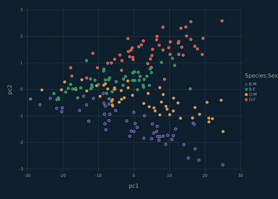
Interestingly, even though the second and third principal components explain a total of 1.61% of the variation in the data, they give very good separation of the four classes in the crabs dataset; in fact, they give much better separation of the classes than the first two principal components (Figures 6.1 and 6.2). This example illustrates that principal components that explain the vast majority of the variation within data still might be missing important information about subpopulations or, perhaps unknown, classes.

6.3  PROBABILISTIC PRINCIPAL COMPONENTS ANALYSIS

Probabilistic principal components analysis (PPCA; Tipping and Bishop, 1999b) is a data reduction technique that replaces p observed variables by q < p latent components. The method works well when the q latent components explain a satisfactory amount of the variability in the p observed variables. In some situations, we might even have substantial dimension reduction, i.e., q ≪ p. There are interesting relationships between PPCA and principal components analysis and, indeed, between PPCA and factor analysis (Spearman, 1904, 1927) — these relationships will be discussed later. In what follows, the notation and approach are similar to those used by McNicholas (2016a).

Consider independent p-dimensional random variables X₁, …, X_n. The PPCA model can be written

$X_i=\mathit{\mu }+\Lambda U_i+{\mathit{ϵ}}_i,$

(6.6)

Figure 6.1 Scallerplot depicting the first two principal components for the crabs data, coloured by class.

Figure 6.2 Scallerplot depicting the second and third principal components for the crabs data, coloured by class.

for i = 1, …, n, where Λ is a p × q matrix of component (or factor) loadings, the latent component $U_i\sim \mathcal{N}\left(0,I_q\right)$, and ${ϵ}_i\sim \mathcal{N}\left(0,\phi I_p\right)$, where ψ ∈ ℝ⁺. Note that the U_i are independently distributed and independent of the ϵ_i, which are also independently distributed. From (6.6), it follows that the marginal distribution of X_i under the PPCA model is $\mathcal{N}\left(\mathit{\mu },\mathbf{\Lambda }{\mathbf{\Lambda }}^{\prime }+\psi I_p\right)$ There are

$pq-\frac{1}{2}q\left(q-1\right)+1$

free parameters in the covariance matrix ΛΛ′ + ψΙ_p (Lawley and Maxwell, 1962). Therefore, the reduction in free covariance parameters under the PPCA model is

$\frac{1}{2}p\left(p+1\right)-\left[pq-\frac{1}{2}q\left(q-2\right)+1\right]=\frac{1}{2}\left[{\left(p-q\right)}^2+p-q-2\right],$

(6.7)

and there is a reduction in the number of free parameters provided that (6.7) is positive, i.e., provided that

${\left(p-q\right)}^2>q-p+2.$

The log-likelihood for p-dimensional x₁, x₂, …, x_n from the PPCA model is

$\begin{array}{l}l\left(\mu ,\Lambda ,\Psi \right)={\displaystyle \sum _{i=1}^{n}log\varphi }\left(x_i|\mathit{\mu },\Lambda {\Lambda }^{\prime }+\psi I_p\right)\\ =-\frac{np}{2}log2\pi -\frac{n}{2}log\left|\Lambda {\Lambda }^{\prime }+\psi I_p\right|-\frac{n}{2}\text{tr}\left\{S{\left(\Lambda {\Lambda }^{\prime }+\psi I_p\right)}^{-1}\right\},\end{array}$

(6.8)

where

$S=\frac{1}{n}{\displaystyle \sum _{i=1}^n\left(x_i-\mathit{\mu }\right){\left(x_i-\mu \right)}^{\prime }}.$

(6.9)

The maximum likelihood estimate for μ is easily obtained by differentiating (6.8) with respect to μ and setting the resulting score function equal to zero to get $\widehat{\mu }=\text{X}¯$. An EM algorithm can be used to obtain maximum likelihood estimates for Λ and Ψ.

6.4  EM ALGORITHM FOR PPCA

6.4.1  Background: EM Algorithm

The expectation-maximization (EM) algorithm (Dempster et al., 1977) is an iterative procedure for finding maximum likelihood estimates when data are incomplete or treated as such. The EM algorithm iterates between an E-step and an M-step until some stopping rule is reached. On the E-step, the expected value of the complete-data log-likelihood is computed conditional on the current parameter estimates. On the M-step, this quantity is maximized with respect to the parameters to obtain (new) updates. Extensive details on the EM algorithm are provided by McLachlan and Krishnan (2008).

6.4.2  E-step

The complete-data comprise the observed x₁, …, x_n together with the latent components u₁, …, u_n, where $u_i={\left(u_{i1},\dots ,u_{iq}\right)}^{\prime }$. Now, noting that $X_i|u_i\sim \mathcal{N}\left(\mu ,+\Lambda u_i,\phi I_p\right)$, we have

$\begin{array}{l}logf\left(x_i|u_i\right)=-\frac{p}{2}log2\pi -\frac{1}{2}log\left|\psi I_p\right|\\ -\frac{1}{2}{\left(x_i-\mu -\Lambda u_i\right)}^{\prime }{\left(\psi I_p\right)}^{-1}\left(x_i-\mu -\Lambda u_i\right)\\ =-\frac{p}{2}log2\pi -\frac{p}{2}log\psi -\frac{1}{2\psi }[{\left(x_i-\mu \right)}^{\prime }\left(x_i-\mu \right)+{\left(x_i-\mu \right)}^{\prime }\Lambda u_i\\ +{u^{\prime }}_i{\Lambda }^{\prime }\left(x_i-\mu \right)-{u^{\prime }}_i{\Lambda }^{\prime }\Lambda u_i]\\ =-\frac{p}{2}log2\pi -\frac{p}{2}log\psi -\frac{1}{2\psi }\text{tr}\left\{\left(x_i-\mu \right){\left(x_i-\mu \right)}^{\prime }\right\}\\ +\frac{1}{\psi }\text{tr}\left\{{\left(x_i-\mu \right)}^{\prime }\Lambda u_i\right\}-\frac{1}{2\psi }\text{tr}\left\{{\Lambda }^{\prime }\Lambda u_i{u^{\prime }}_i\right\}.\end{array}$

Now, the complete-data log-likelihood can be written

$\begin{array}{l}{l}_{\text{c}}\left(\mu ,\Lambda ,\Psi \right)={\displaystyle \sum _{i=1}^{n}log}\left[f\left(x_i|u_i\right)f\left(u_i\right)\right]\\ =C-\frac{np}{2}log\psi -\frac{1}{2\psi }\text{tr}\left\{{\displaystyle \sum _{i=1}^n\left(x_i-\mu \right){\left(x_i-\mu \right)}^{\prime }}\right\}\\ +\frac{1}{\psi }{\displaystyle \sum _{i=1}^n\text{tr}}\left\{{\left(x_i-\mu \right)}^{\prime }\Lambda u_i\right\}-\frac{1}{2\psi }\text{tr}\left\{{\Lambda }^{\prime }\Lambda {\displaystyle \sum _{i=1}^n{\text{u}}_i{\text{u}}_i{}^{\prime }}\right\},\end{array}$

where C is constant with respect to μ, Λ, and ψ.

Consider the joint distribution

$\left[\begin{array}{c}{X}_i\\ U_i\end{array}\right]\sim \mathcal{N}\left(\left[\begin{array}{c}\mu \\ 0\end{array}\right],\left[\begin{array}{cc}\Lambda {\Lambda }^{\prime }+\psi I_p& \Lambda \\ {\Lambda }^{\prime }& I_q\end{array}\right]\right).$

It follows that

$\mathbb{E}\left[{\text{U}}_i|{\text{x}}_i\right]=\beta \left({\text{x}}_i-\mu \right),$

(6.10)

where β = Λ′(ΛΛ′ + ψΙp)⁻¹, and

$\begin{array}{c}\mathbb{E}\left[{\text{U}}_i{\text{U}}_i{}^{\prime }|{\text{x}}_i\right]=\mathbb{V}\text{ar}\left[{\text{U}}_i|{\text{x}}_i\right]+\mathbb{E}\left[{\text{U}}_i|{\text{x}}_i\right]\mathbb{E}{\left[{\text{U}}_i|{\text{x}}_i\right]}^{\prime }\\ ={\text{I}}_q-\beta \Lambda +\beta \left({\text{x}}_i-\mu \right){\left({\text{x}}_i-\mu \right)}^{\prime }{\beta }^{\prime }.\end{array}$

(6.11)

Therefore, noting that $\widehat{\mu }=\overline{\text{x}}$ and that we are conditioning on the current parameter estimates, the expected value of the complete-data log-likelihood can be written

$\begin{array}{l}Q\left(\Lambda ,\psi \right)=C-\frac{np}{2}log\psi -\frac{1}{2\psi }\text{tr}\left\{{\displaystyle \sum _{i=1}^n\left({\text{x}}_i-\overline{\text{x}}\right){\left({\text{x}}_i-\overline{\text{x}}\right)}^{\prime }}\right\}\\ +\frac{1}{\psi }{\displaystyle \sum _{i=1}^n\text{tr}\left\{{\left({\text{x}}_i-\overline{\text{x}}\right)}^{\prime }\Lambda \mathbb{E}\left[{\text{U}}_i\left|{\text{x}}_i\right|\right]\right\}}\\ -\frac{1}{2\psi }\text{tr}\left\{{\Lambda }^{\prime }\Lambda {\displaystyle \sum _{i=1}^n\mathbb{E}\left[{\text{U}}_i{\text{U}}_i{}^{\prime }|{\text{x}}_i,\right]}\right\}\\ =C-\frac{np}{2}log\psi -\frac{n}{2\psi }\text{tr}\left\{{\text{S}}_{\overline{\text{x}}}\right\}+\frac{n}{\psi }\text{tr}\left\{\Lambda \widehat{\beta }\text{S}\overline{\text{x}}¯\right\}-\frac{n}{2\psi }\text{tr}\left\{{\Lambda }^{\prime }\Lambda \Theta \right\},\end{array}$

where $\Theta ={\text{I}}_q-\widehat{\beta }\widehat{\Lambda }+\widehat{\beta }{S}_{\overline{\text{x}}}{\widehat{\beta }}^{\prime }$ is a symmetric q × q matrix, $\widehat{\beta }={\widehat{\Lambda }}^{\prime }{\left(\widehat{\Lambda }{\widehat{\Lambda }}^{\prime }+\widehat{\phi }{\text{I}}_p\right)}^{-1}$, and

${\text{S}}_{\overline{\text{x}}}=\frac{1}{n}{\displaystyle \sum _{i=1}^n\left({\text{x}}_i-\overline{\text{x}}\right)}{\left({\text{x}}_i-\overline{\text{x}}\right)}^{\prime }$

(6.12)

can be thought of as the sample, or observed, covariance matrix.

6.4.3  M-step

Differentiating Q with respect to Λ and ψ, respectively, gives the score functions

$\begin{array}{ll}{S}_1(\mathbf{\Lambda },\psi )=\frac{\partial Q}{\partial \mathbf{\Lambda }}\hfill & =\frac{n}{\psi }\frac{\partial }{\partial \mathbf{\Lambda }}\text{tr}\left\{\mathbf{\Lambda }\widehat{\beta }{S}_{\overline{x}}\right\}-\frac{n}{2\psi }\frac{\partial }{\partial \mathbf{\Lambda }}\text{tr}\{{\mathbf{\Lambda }}^{\prime }\mathbf{\Lambda }\Theta \}\hfill \\ \hfill & =\frac{n}{\psi }{S}^{\prime }{}_{\overline{x}}{\widehat{\beta }}^{\prime }-\frac{n}{2\psi }(2\mathbf{\Lambda }\Theta )=\frac{n}{\psi }(S_{\overline{x}}{\widehat{\beta }}^{\prime }-\mathbf{\Lambda }\Theta ),\hfill \end{array}$

and

$\begin{array}{ll}{S}_2(\mathbf{\Lambda },\psi )\hfill & =\frac{\partial Q}{\partial {\psi }^{-1}}\hfill \\ \hfill & =\frac{np\psi }{2}-\frac{n}{2}\text{tr}\left\{S_{\overline{x}}\right\}+n\text{tr}\left\{\mathbf{\Lambda }\widehat{\beta }{S}_{\overline{x}}\right\}\frac{n}{2}\text{tr}\{{\mathbf{\Lambda }}^{\prime }\mathbf{\Lambda }\Theta \}\hfill \\ \hfill & =\frac{n}{2}\left(p\psi -\text{tr}\{S_{\overline{x}}-2\mathbf{\Lambda }\widehat{\beta }{S}_{\overline{x}}+{\mathbf{\Lambda }}^{\prime }\mathbf{\Lambda }\Theta \}\right).\hfill \end{array}$

Solving the equations $S_1\left({\widehat{\Lambda }}^{\text{new}},{\widehat{\phi }}^{\text{new}}\right)=0$ and $S_2\left({\widehat{\Lambda }}^{\text{new}},{\widehat{\phi }}^{\text{new}}\right)=0$ gives

$\begin{array}{ll}{\widehat{\mathbf{\Lambda }}}^{\text{new}}\hfill & =S_{\overline{x}}{\widehat{\beta }}^{\prime }{\Theta }^{-1}\hfill \\ {\widehat{\psi }}^{\text{new}}\hfill & =\frac{1}{p}\text{tr}\{S_{\overline{x}}-2{\widehat{\mathbf{\Lambda }}}^{\text{new}}\widehat{\beta }{S}_{\overline{x}}+{({\widehat{\mathbf{\Lambda }}}^{\text{new}})}^{\prime }{\widehat{\mathbf{\Lambda }}}^{\text{new}}\Theta \}\hfill \\ \hfill & =\frac{1}{p}\text{tr}\{S_{\overline{x}}-2{\widehat{\mathbf{\Lambda }}}^{\text{new}}\widehat{\beta }{S}_{\overline{x}}+{(S_{\overline{x}}\widehat{\beta }{\Theta }^{-1})}^{\prime }{\widehat{\mathbf{\Lambda }}}^{\text{new}}\Theta \}\hfill \\ \hfill & =\frac{1}{p}\text{tr}\{S_{\overline{x}}-{\widehat{\mathbf{\Lambda }}}^{\text{new}}\widehat{\beta }{S}_{\overline{x}}\}.\hfill \end{array}$

The matrix results used to compute these score functions, and used elsewhere in this section, are listed in Appendix C.

6.4.4  Woodbury Identity

On each iteration of the EM algorithm for PPCA, the p × p matrix ${\left(\widehat{\Lambda }{\widehat{\Lambda }}^{\prime }+\widehat{\phi }{\text{I}}_p\right)}^{-1}$ needs to be computed. Computing this matrix inverse can be computationally expensive, especially for larger values of p. The Woodbury identity (Woodbury, 1950) can be used in such situations to avoid inversion of non-diagonal p × p matrices. For an m × m matrix A, an m × k matrix U, a k × k matrix C, and a k × m matrix V, the Woodbury identity is

${\left(A+UCV\right)}^{-1}=A^{-1}-A^{-1}U{\left(C^{-1}+V{A}^{-1}U\right)}^{-1}V{A}^{-1}.$

Setting $\mathbf{U}=\widehat{\mathbf{\Lambda }}$, $\mathbf{V}={\widehat{\mathbf{\Lambda }}}^{\prime }$,$\mathbf{A}=\widehat{\phi }{\mathbf{I}}_p$, and C = I_q gives

$\begin{array}{ll}{(\widehat{\psi }{I}_p+\widehat{\mathbf{\Lambda }}{\widehat{\mathbf{\Lambda }}}^{\prime })}^{-1}\hfill & =\frac{1}{\widehat{\psi }}{I}_p-\frac{1}{\widehat{\psi }}\mathbf{\Lambda }{(I_q+\frac{1}{\widehat{\psi }}{\widehat{\mathbf{\Lambda }}}^{\prime }\widehat{\mathbf{\Lambda }})}^{-1}{\widehat{\mathbf{\Lambda }}}^{\prime }\frac{1}{\widehat{\psi }}\hfill \\ \hfill & =\frac{1}{\widehat{\psi }}{I}_p-\frac{1}{\widehat{\psi }}\mathbf{\Lambda }{(\widehat{\psi }{I}_q+\mathbf{\Lambda }{\mathbf{\Lambda }}^{\prime })}^{-1}{\mathbf{\Lambda }}^{\prime },\hfill \end{array}$

(6.13)

which can be used to speed up the EM algorithm for the PPCA model. The left-hand side of (6.13) requires inversion of a p × p matrix but the right-hand side leaves only a q × q matrix and some diagonal matrices to be inverted. A related identity for the determinant of the covariance matrix,

$\begin{array}{l}\begin{array}{c}\begin{array}{l}\begin{array}{ll}|\widehat{\mathbf{\Lambda }}{\widehat{\mathbf{\Lambda }}}^{\prime }+\widehat{\psi }{I}_p|\hfill & =\frac{\left|\widehat{\psi }{I}_p\right|}{|I_p-{\mathbf{\Lambda }}^{\prime }{(\mathbf{\Lambda }{\mathbf{\Lambda }}^{\prime }+\widehat{\psi }{I}_p)}^{-1}\mathbf{\Lambda }|}\hfill \\ \hfill & =\frac{{\widehat{\psi }}^p}{|I_p-{\mathbf{\Lambda }}^{\prime }{(\mathbf{\Lambda }{\mathbf{\Lambda }}^{\prime }+\widehat{\psi }{I}_p)}^{-1}\mathbf{\Lambda }|},\hfill \end{array}\\ \end{array}\\ \end{array}\hfill \\ \hfill \end{array}$

(6.14)

is also helpful in computation of the component densities. Identities (6.13) and (6.14) give an especially significant computational advantage when p is large and q ≪ p.

6.4.5  Initialization

Similar to McNicholas and Murphy (2008), the parameters $\widehat{\Lambda }$ and $\widehat{\phi }$ can be initialized in several ways, including via eigendecomposition of $S_{\overline{\text{x}}}$. Specifically, $S_{\overline{\text{x}}}$ is computed and then it is eigen-decomposed to give

$S_{\overline{\text{x}}}=PD{P}^{-1},$

and $\widehat{\Lambda }$ is initialized using

$\widehat{\Lambda }=dP,$

where d is the element-wise square root of the diagonal of D. The initial value of ψ can be taken to be

$\widehat{\psi }=\frac{1}{p}\text{tr}\left\{S_{\overline{\text{x}}}-\left(dP\right){\left(dP\right)}^{\prime }\right\}.$

6.4.6  Stopping Rule

There are several options for stopping an EM algorithm. One popular approach is to stop an EM algorithm based on lack of progress in the log-likelihood, i.e., stopping the algorithm when

$l^{\left(k+1\right)}-l^{\left(k\right)}<ϵ,$

(6.15)

for ϵ small, where l^(k) is the (observed) log-likelihood value from iteration k. This stopping rule can work very well when the log-likelihood increases and then plateaus at the maximum likelihood estimate. However, likelihood values do not necessarily behave this way and so it can be worth considering alternatives — see Chatper 2 of McNicholas (2016a) for an illustrated discussion.

As McNicholas (2016a) points out, Böhning et al. (1994), Lindsay (1995), and McNicholas et al. (2010) consider convergence criteria based on Aitken’s acceleration Aitken (1926). Aitken’s acceleration at iteration k is

$a^{\left(k\right)}=\frac{l^{\left(k+1\right)}-l^{\left(k\right)}}{l^{\left(k\right)}-l^{\left(k-1\right)}},$

(6.16)

and an asymptotic estimate of the log-likelihood at iteration k + 1 can be computed via

$l_{\infty }^{\left(k+1\right)}=l^{\left(k\right)}+\frac{l^{\left(k+1\right)}-l^{\left(k\right)}}{1-a^{\left(k\right)}}.$

(6.17)

Note that “asymptotic” here refers to the iteration number so that (6.17) can be interpreted as an estimate, at iteration k + 1, of the ultimate value of the log-likelihood. Following McNicholas et al. (2010), the algorithm can be considered to have converged when

$0<l_{\infty }^{\left(k+1\right)}-l^{\left(k\right)}<ϵ.$

(6.18)

6.4.7  Implementing the EM Algorithm for PPCA

The EM algorithm for PPCA is implemented in two steps. First, we define some helper functions in the following code block. They are used by the EM algorithm function. Specifically, we have implemented a function for each of the identities (6.13) and (6.14) along with functions for each of the equations (6.8) and (6.16). Doing this helps keep the code modular, which facilitates testing some of the more complex mathematics in the algorithm.

## EM Algorithm for PPCA -- Helper functions

function wbiinv(q, p, psi, L)

 ## Woodbury Indentity eq 6.13

 Lt = transpose(L)

 Iq = Matrix{Float64}(I, q, q)

 Ip = Matrix{Float64}(I, p, p)

 psi2 = /(1, psi)

 m1 = *(psi2, Ip)

 m2c = +(*(psi, Iq), *(Lt, L))

 m2 = *(psi2, L, inv(m2c), Lt)

 return(-(m1, m2))

end

function wbidet(q, p, psi, L)

 ## Woodbury Indentity eq 6.14

 Iq = Matrix{Float64}(I, q, q)

 num = psi^p

 denl = *(transpose(L), wbiinv(q, p, psi, L), L)

 den = det(-(Iq, den1))

 return(/(num, den))

end

function ppca_ll(n, q, p, psi, L, S)

 ## log likelihood eq 6.8

 n2 = /(n, 2)

 c = /(*(n, p, log(*(2, pi))), 2)

 l1 = *(n2, log(wbidet(q, p, psi, L)))

 l2 = *(n2, tr(*(S, wbiinv(q, p, psi, L))))

 return(*(-1,+(c, l1, l2)))

end

function cov_mat(X)

 n,p = size(X)

 mux = mean(X, dims = 1)

 X_c = .-(X, mux)

 res = *(/(1,n), *(transpose(X_c), X_c))

 return(res)

end

function aitkenaccel(l1, l2, l3, tol)

 ## l1 = l(k+1), l2 = l(k), l3 = l(k-1)

 conv = false

 num = -(l1,l2)

 den = -(l2, l3)

 ## eq 6.16

 ak = /(num, den)

 if ak <= 1.0

  c1 = -(l1, l2)

  c2 = -(1.0, ak)

  ## eq 6.17

  l_inf = +(l2, /(c2, c1))

  c3 = -(l_inf, l2)

  if 0.0 < c3 < tol

   conv = true

  end

 end

 return conv

end

function ppca_fparams(p, q)

 ## number of free parameters in the ppca model

 c1 = *(p, q)

 c2 = *(-1,q, -(q, 1), 0.5)

 return(+(c1, c2, 1))

end

function BiC(ll, n, q, ρ)

 ## name does not conflict with StatsBase

 ## eq 6.19

 c1 = *(2, ll)

 c2 = *(ρ,log(n))

 return(-(c1, c2))

end

The ppca() function, illustrated in the following code block, carries out the EM algorithm described previously. It uses the eigen-decomposition of the sample covariance matrix to initialize Λ, which is used in turn to initialize ψ. A while loop is used to iteratively perform the (post-) E-step updates for β and Θ as well as the M-step updates of Λ and ψ. After the M-step, the log-likelihood is calculated and its value is stored in an array. The values in the array are used to calculate the Aitken acceleration to check convergence. The Woodbury identity is used to speed up the beta updates and the log-likelihood computations. The function returns a Julia dictionary with the PPCA results. The results include the number of iterations the EM algorithm ran, the array of log-likelihoods, the model parameters, the number of latent components q, the standard deviations from the eigen-decomposition, the orthonormal coefficients, and the projections of the data onto the latent space.

using LinearAlgebra, Random

Random.seed!(429)

include("chp6_ppca_functions.jl")

## EM Function for PPCA

function ppca(X; q = 2, thresh = 1e-5, maxit = 1e5)

  Iq = Matrix{Float64}(I, q, q)

  qI = *(q, Iq)

  n,p = size(X)

  ## eigfact has eval/evec smallest to largest

  ind = p:-1:(p-q+1)

  Sx = cov_mat(X)

  D = eigen(Sx)

  d = diagm(0 => map(sqrt, D.values[ind]))

  P = D.vectors[:, ind]

  ## initialize parameters

  L = *(P, d) ## pxq

  psi = *(/(1,p), tr(-(Sx, *(L, transpose(L)))))

  B = zeros(q,p)

  T = zeros(q,q)

  conv = true

  iter = 1

  ll = zeros(100)

  ll[1] = 1e4

 ## while not converged

 while(conv)

  ## above eq 6.12

  B = *(transpose(L), wbiinv(q, p, psi, L)) ## qxp

  T = -(qI, +(*(B,L), *(B, Sx, transpose(B)))) ## qxq

  ## sec 6.4.3 - update Lambda_new

  L_new = *(Sx, transpose(B), inv(T)) ## pxq

  ## update psi_new

  psi_new = *(/(1,p), tr(-(Sx, *(L_new, B, Sx)))) #num

  iter += 1

  if iter > maxit

    conv = false

    println("ppca() while loop went over maxit parameter. iter =

      $iter")

  else

    ## stores at most the 100 most recent ll values

    if iter <= 100

     ll[iter]=ppca_ll(n, q, p, psi_new, L_new, Sx)

    else

     ll = circshift(ll, -1)

     ll[100] = ppca_ll(n, q, p, psi_new, L_new, Sx)

    end

    if 2 < iter < 101

      ## scales the threshold by the latest ll value

      thresh2 = *(-1,ll[iter], thresh)

      if aitkenaccel(ll[iter], ll[(iter-1)], ll[(iter-2)], thresh2)

        conv = false

      end

    else

      thresh2 = *(-1,ll[100], thresh)

      if aitkenaccel(ll[100], ll[(99)], ll[(98)], thresh2)

       conv = false

      end

    end

  end ## if maxit

  L = L_new

  psi = psi_new

 end ## while

 ## orthonormal coefficients

 coef = svd(L).U

 ## projections

 proj = *(X, coef)

 if iter <= 100

  resize!(ll, iter)

 end

 fp = ppca_fparams(p, q)

 bic_res = BiC(ll[end], n, q, fp)

 return(Dict(

   "iter" => iter,

   "ll" => ll,

   "beta" => B,

   "theta" => T,

   "lambda" => L,

   "psi" => psi,

   "q" =>

   "sd" => diag(d),

   "coef" => coef,

   "proj" => proj,

   "bic" => bic_res

  ))

end

ppca1 = ppca(crab_mat_c, q=3, maxit = 1e3)

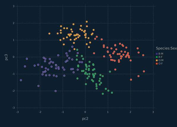
It should be noted that the Λ matrix is neither orthonormal nor composed of eigenvectors (Tipping and Bishop, 1999b). To get orthonormal principal components from it, a singular value decomposition is performed on Λ and the left singular vectors are used as principal component loadings. The projections are plotted in Figure 6.3. With three latent components, we see a clear separation between the crab species.

Figure 6.3 Scallerplot depicting the second and third principal components from the PPCA model with three latent components for the crabs data, coloured by sex and species.

6.4.8  Comments

The choice of the number of latent components is an important consideration in PPCA. One approach is to choose the number of latent components that captures a certain proportion of the variation in the data. Lopes and West (2004) carry out simulation studies showing that the Bayesian information criterion (BIC; Schwarz, 1978) can be effective for selection of the number of latent factors in a factor analysis model, and a similar approach can be followed for PPCA. The BIC is given by

$\text{BIC}=2l\left(\widehat{\vartheta }\right)-\rho logn,$

(6.19)

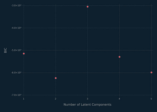
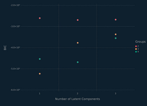
where $\widehat{\vartheta }$ is the maximum likelihood estimate of $\vartheta$,$l\left(\widehat{\vartheta }\right)$ is the maximized (observed) log-likelihood, and ρ is the number of free parameters in the model. The BIC values for PPCA models with different numbers of latent components run on the crabs data are displayed in figure 6.4. The clear choice is the model with three latent components, which has the largest BIC value based on equation 6.19. Clearly this model is capturing the important information in the third principal component, visualized in figure 6.3.

Figure 6.4 BIC values for the PPCA models with different numbers of latent components for the crabs data.

The goal of PPCA is not to necessarily give better results than PCA, but to permit a range of extensions. The probabilistic formulation of the PPCA model allows these extensions, one of which will be illustrated in Section 6.6. Because the PPCA model has a likelihood formulation, it can easily be compared to other probabilistic models, it may be formulated to work with missing data, and adapted for use as a Bayesian method. Noted that, as ψ → 0, the PPCA solution converges to the PCA solution (see Tipping and Bishop, 1999b, for details).

6.5  K-MEANS CLUSTERING

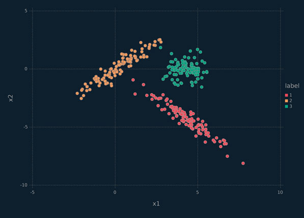
The k-means clustering technique iteratively finds k cluster centres and assigns each observation to the nearest cluster centre. For k-means clustering, these cluster centres are simply the means. The result of k-means clustering is effectively to fit k circles of equal radius to data, where each circle centre corresponds to one of the k means. Of course, for p > 2 dimensions, we have p-spheres rather than circles. Consider the k-means clustering of the x2 data in the following code block. Recall that the x2 data is just a mixture of three bivariate Gaussian distributions (Figure 6.5).

Figure 6.5 Scallerplot depicting the x2 data, coloured by class.

The x2 data present an interesting example of simulated data where classes from the generative model, i.e., a three-component Gaussian mixture model, cannot quite be taken as the correct result. Specifically, an effective clustering procedure would surely put one of the green-coloured points in Figure 6.5 in the same cluster as the yellow points.

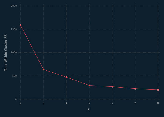
In the following code block, the choice of k is made using the elbow method, where one plots k against the total cost, i.e., the total within-cluster sum of squares, and chooses the value of k corresponding to the “elbow” in the plot. Note that the total within-cluster sum of squares is

${\displaystyle \sum _{g=1}^k{\displaystyle \sum _{{\text{x}}_i\in C_g}{\left({\text{x}}_i-{\overline{\text{x}}}_g\right)}^2,}}$

where C_g is the gth cluster and ${\overline{x}}_g$ is its mean.

using DataFrames, Clustering, Gadfly, Random

Random.seed!(429)

mean_x2 = mean(x2_mat, dims=1)

## mean center the cols

x2_mat_c = x2_mat .- mean_x2

N = size(x2_mat_c)[1]

## kmeans() - each column of X is a sample - requires reshaping x2

x2_mat_t = reshape(x2_mat_c, (2,N))

## Create data for elbow plot

k = 2:8

df_elbow = DataFrame(k = Vector{Int64}(), tot_cost = Vector{Float64}())

for i in k

  tmp = [i, kmeans(x2_mat_t, i; maxiter=10, init=:kmpp).totalcost ]

  push!(df_elbow, tmp)

end

## create elbow plot

p_km_elbow = plot(df_elbow, x = :k, y = :tot_cost, Geom.point, Geom.line,

 Guide.xlabel("k"), Guide.ylabel("Total Within Cluster SS"),

 Coord.Cartesian(xmin = 1.95), Guide.xticks(ticks = collect(2:8)))

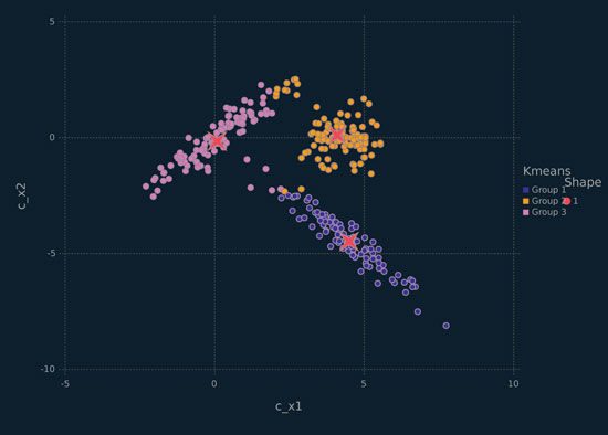
From Figure 6.6, it is clear that the elbow occurs at k = 3. The performance of k-means clustering on this data is not particularly good (Figure 6.7), which is not surprising. The reason this result is not surprising is that, as mentioned before, k-means clustering will essentially fit k circles — for the x2 data, two of the three clusters are long ellipses.

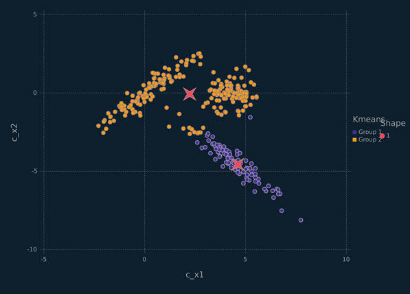
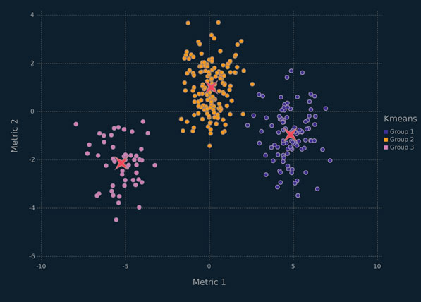
It is of interest to consider the solution for k = 2 (Figure 6.8) because it further illustrates the reliance of k-means clustering on clusters that are approximately circles. An example where k-means should, and does, work well is shown in Figure 6.9, where the clusters are well described by fitted circles of equal radius. It is also worth noting that k-means clustering works well for trivial clustering problems where there is significant spatial separation between each cluster, regardless of the cluster shapes.

Figure 6.6 Elbow plot for selecting k in the k-means clustering of the x2 data.

Figure 6.7 Scallerplot depicting the x2 data, coloured by the k-means clustering solution for k = 3, with red stars marking the cluster means.

Figure 6.8 Scallerplot depicting the x2 data, coloured by the k-means clustering solution for k = 2, with red stars marking the cluster means.

Figure 6.9 Scallerplot depicting a dataset where k-means works well, coloured by the k-means clustering solution for k = 3, with red stars marking the cluster means.

6.6  MIXTURE OF PROBABILISTIC PRINCIPAL COMPONENTS ANALYZERS

6.6.1  Model

Building on the PPCA model, Tipping and Bishop (1999a) introduced the the mixture of probabilistic principal components analyzers (MPPCA) model. It can model complex structures in a dataset using a combination of local PPCA models. As PPCA provides a reduced dimensional representation of the data, MPPCA models work well in high-dimensional clustering, density estimation and classification problems.

Analogous to the PPCA model (Section 6.3), the MPPCA model assumes that

$X_i={\mu }_g+{\Lambda }_g{U}_{ig}+{ϵ}_{ig}$

(6.20)

with probability π_g, for i = 1, …, n and g = 1, …, G, where Λ_g is a p × q matrix of loadings, the U_ig are independently N(0, I_q) and are independent of the ϵ_ig, which are independently N(0, ψ₉I_p), where ψ_g ∈ ℝ⁺. It follows that the density of X_i from the MPPCA model is

$f\left(x_i|\vartheta \right)={\displaystyle \sum _{g=1}^G{\pi }_g\varphi \left(x_i|{\mu }_g,{\Lambda }_g{{\Lambda }^{\prime }}_g+{\psi }_g{I}_p\right),}$

(6.21)

where ϑ denotes the model parameters.

6.6.2  Parameter Estimation

Overview

Parameter estimation for the MPPCA model can be carried out using an alternating expectation-conditional maximization (AECM) algorithm (Meng and van Dyk, 1997). The expectation-conditional maximization (ECM) algorithm (Meng and Rubin, 1993) is a variant of the EM algorithm that replaces the M-step by a series of conditional maximization steps. The AECM algorithm allows a different specification of complete-data for each conditional maximization step. Accordingly, the AECM algorithm is suitable for the MPPCA model, where there are two sources of missing data: the unknown component membership labels and the latent components (or factors) u_ig, for i = 1, …,n and g = 1, …,G. Details of fitting the AECM algorithm for the more general mixture of factor analyzers model are given by McLachlan and Peel (2000), and parameter estimation for several related models is discussed by McNicholas and Murphy (2008, 2010) and McNicholas et al. (2010).

AECM Algorithm: First Stage

As usual, denote by z₁, …, z_n the unobserved component membership labels, where $z_{ig}=1$ if observation i belongs to component g and $z_{ig}=0$ otherwise. At the first stage of the AECM algorithm, the complete-data are taken to be the observed x₁, …, x_n together with the unobserved z₁, …, z_n, and the parameters π_g and µ_g are estimated, for g = 1, …, G. The complete-data log-likelihood is

$l_1={\displaystyle \sum _{i=1}^n{\displaystyle \sum _{g=1}^G{z}_{ig}log\left[{\pi }_g\varphi \left(x_i|{\mu }_g,{\Lambda }_g{{\Lambda }^{\prime }}_g+{\psi }_g{I}_p\right)\right]},}$

(6.22)

and the (conditional) expected values of the component membership labels are given by

${\widehat{z}}_{ig}=\frac{{\widehat{\pi }}_g\varphi \left(x_i|{\widehat{\mu }}_g,{\widehat{\Lambda }}_g{\widehat{{\Lambda }^{\prime }}}_g+{\widehat{\psi }}_g{I}_p\right)}{{\displaystyle \sum {}_{h=1}^G}{\widehat{\pi }}_h\varphi \left(x_i|{\widehat{\mu }}_g,{\widehat{\Lambda }}_h{\widehat{{\Lambda }^{\prime }}}_h+{\widehat{\psi }}_h{I}_p\right)},$

(6.23)

for i = 1, …, n and g = 1, …, G.

Using the expected values given by (6.23) within (6.22), the expected value of the complete-data log-likelihood at the first stage is

$\begin{array}{ll}{Q}_1\hfill & ={\displaystyle \sum }_{i=1}^n{\displaystyle \sum }_{g=1}^G{\widehat{z}}_{ig}[log{\pi }_g+log\varphi (x_i|{\mu }_g,{\mathbf{\Lambda }}_g{\mathbf{\Lambda }}^{\prime }{}_g+{\psi }_g{I}_p)]\hfill \\ \hfill & ={\displaystyle \sum }_{g=1}^G{n}_{g}log{\pi }_g-\frac{np}{2}log2\pi -{\displaystyle \sum }_{g=1}^G\frac{n_g}{2}log|{\mathbf{\Lambda }}_g{\mathbf{\Lambda }}^{\prime }{}_g+{\psi }_g{I}_p|-{\displaystyle \sum }_{g=1}^G\frac{n_g}{2}\text{tr}\left\{S_g{({\mathbf{\Lambda }}_g{\mathbf{\Lambda }}^{\prime }{}_g+{\psi }_g{I}_p)}^{-1}\right\},\hfill \end{array}$

where $n_g={\displaystyle \sum {}_{i=1}^n}{\widehat{z}}_{ig}$ and

$S_g=\frac{1}{n_g}{\displaystyle \sum _{i=1}^n{\widehat{z}}_{ig}\left({\text{x}}_i-{\mu }_g\right){\left({\text{x}}_i-{\mu }_g\right)}^{\prime }}.$

(6.24)

Maximising Q₁ with respect to π_g and µ_g yields

$\begin{array}{ccc}{\widehat{\pi }}_g=\frac{n_g}{n}& \text{and}& {\widehat{\mu }}_g=\frac{{\displaystyle \sum {}_{i=1}^n}{\widehat{z}}_{ig}{\text{x}}_i}{{\displaystyle \sum {}_{i=1}^n}{\widehat{z}}_{ig}}\end{array},$

(6.25)

respectively.

AECM Algorithm: Second Stage

At the second stage of the AECM algorithm, the complete-data are taken to be the observed x₁, …,x_n together with the unobserved component membership labels z₁, …,z_n and the latent factors $u_{ig}$, for i = 1, …, n and g = 1, …,G, and the parameters Λ_g and ψ_g are estimated, for g = 1, …, G. Proceeding in an analogous fashion to the EM algorithm for the factor analysis model (Section 6.4), the complete-data log-likelihood is given by

$\begin{array}{ll}{l}_2\hfill & ={\displaystyle \sum }_{i=1}^n{\displaystyle \sum }_{g=1}^G{\widehat{z}}_{ig}[log{\pi }_g+logf(x_i|u_i)+logf(u_i)]\hfill \\ \hfill & =C+{\displaystyle \sum }_{g=1}^G[-\frac{n_{g}p}{2}log{\psi }_g-\frac{n_g}{2{\psi }_g}\text{tr}\{S_g\}\hfill \\ \hfill & +\frac{1}{{\psi }_g}{\displaystyle \sum }_{i=1}^n{z}_{ig}{(x_i-{\mu }_g)}^{\prime }{\Lambda }_g{u}_i-\frac{1}{2{\psi }_g}\text{tr}\left\{{\mathbf{\Lambda }}^{\prime }{}_g{\mathbf{\Lambda }}_g{\displaystyle \sum }_{i=1}^n{z}_{ig}{u}_i{u}^{\prime }{}_i\right\}],\hfill \end{array}$

where C is constant with respect to Λ_g and ψ_g. Bearing in mind that we are conditioning on the current parameter estimates, and using expected values analogous to those in (6.10) and (6.11), the expected value of the complete-data log-likelihood can be written

$\begin{array}{ll}{Q}_2\hfill & =C+{\displaystyle \sum }_{g=1}^G[-\frac{n_{g}p}{2}log{\psi }_g-\frac{n_g}{2{\psi }_g}\text{tr}\{S_g\}\hfill \\ \hfill & +\frac{1}{{\psi }_g}{\displaystyle \sum }_{i=1}^n{\widehat{z}}_{ig}{(x_i-{\widehat{\mu }}_g)}^{\prime }{\mathbf{\Lambda }}_g\mathbb{E}[U_{ig}|x_i,z_{ig}=1]\hfill \\ \hfill & -\frac{1}{2{\psi }_g}\text{tr}\{{\mathbf{\Lambda }}^{\prime }{}_g{\mathbf{\Lambda }}_g{\displaystyle \sum }_{i=1}^n{\widehat{z}}_{ig}\mathbb{E}[U_{ig}{U}^{\prime }{}_{ig}|x_i,z_{ig}=1]\}]\hfill \\ \hfill & =C+\frac{1}{2}{\displaystyle \sum }_{g=1}^G{n}_g[-plog{\psi }_g-\frac{1}{{\psi }_g}\text{tr}\{S_g\}+\frac{2}{{\psi }_g}\text{tr}\{{\mathbf{\Lambda }}_g{\widehat{\beta }}_g{S}_g\}\hfill \\ \hfill & -\frac{1}{{\psi }_g}\text{tr}\left\{{\mathbf{\Lambda }}^{\prime }{}_g{\mathbf{\Lambda }}_g{\Theta }_g\right\}],\hfill \end{array}$

where

${\widehat{\beta }}_g={{\widehat{\Lambda }}^{\prime }}_g{\left({\widehat{\Lambda }}_g{{\widehat{\Lambda }}^{\prime }}_g+{\widehat{\psi }}_g{I}_p\right)}^{-1}$

is a q × p matrix and

${\Theta }_g=I_q-{\widehat{\beta }}_g{\widehat{\Lambda }}_g+{\widehat{\beta }}_g{S}_g{{\widehat{\beta }}^{\prime }}_g$

is a symmetric q × q matrix. Note that ${\widehat{\mu }}_g$ replaces µ_g in S_g, see (6.24).

Differentiating Q₂(Λ, Ψ) with respect to Λ_g and ${\phi }_g^{-1}$, respectively, gives the score functions

$\begin{array}{ll}{S}_1({\mathbf{\Lambda }}_g,{\psi }_g)\hfill & =\frac{\partial Q_2}{\partial {\mathbf{\Lambda }}_g}=\frac{n_g}{{\psi }_g}\frac{\partial }{\partial {\mathbf{\Lambda }}_g}\text{tr}\left\{{\mathbf{\Lambda }}_g{\widehat{\beta }}_g{S}_g\right\}-\frac{n_g}{2{\psi }_g}\frac{\partial }{\partial {\mathbf{\Lambda }}_g}\text{tr}\left\{{\mathbf{\Lambda }}^{\prime }{}_g{\mathbf{\Lambda }}_g{\Theta }_g\right\}\hfill \\ \hfill & =\frac{n_g}{{\psi }_g}{S}^{\prime }{}_g{\widehat{\beta }}^{\prime }{}_g-\frac{n_g}{2{\psi }_g}(2{\mathbf{\Lambda }}_g{\Theta }_g)\hfill \\ \hfill & =\frac{n_g}{{\psi }_g}(S_g{\widehat{\beta }}^{\prime }{}_g-{\mathbf{\Lambda }}_g{\Theta }_g),\hfill \end{array}$

and

$\begin{array}{ll}{S}_2({\mathbf{\Lambda }}_g,{\psi }_g)\hfill & =\frac{\partial Q}{\partial {\psi }_g^{-1}}\hfill \\ \hfill & =\frac{n_{g}p{\psi }_g}{2}-\frac{n_g}{2}\text{tr}\left\{S_g\right\}+n_g\text{tr}\left\{{\mathbf{\Lambda }}_g{\widehat{\beta }}_g{S}_g\right\}-\frac{n_g}{2}\text{tr}\left\{{\mathbf{\Lambda }}^{\prime }{}_g{\mathbf{\Lambda }}_g{\Theta }_g\right\}\hfill \\ \hfill & =\frac{n_g}{2}(p{\psi }_g-\text{tr}\{S_g-2{\mathbf{\Lambda }}_g{\widehat{\beta }}_g{S}_g+{\mathbf{\Lambda }}^{\prime }{}_g{\mathbf{\Lambda }}_g{\Theta }_g\}).\hfill \end{array}$

Solving the equations $S_1\left({\widehat{\Lambda }}_g^{\text{new}},{\widehat{\phi }}_g^{\text{new}}\right)=0$ and $S_2\left({\widehat{\Lambda }}_g^{\text{new}},{\widehat{\phi }}_g^{\text{new}}\right)=0$ gives

$\begin{array}{ll}{\widehat{\mathbf{\Lambda }}}_g^{\text{new}}\hfill & =S_g{\widehat{\beta }}^{\prime }{}_g{\Theta }_g^{-1}\hfill \\ {\widehat{\psi }}_g^{\text{new}}\hfill & =-\frac{1}{p}\text{tr}\{S_g-2{\widehat{\mathbf{\Lambda }}}_g^{\text{new}}{\widehat{\beta }}_g{S}_g+{({\widehat{\mathbf{\Lambda }}}_g^{\text{new}})}^{\prime }{\widehat{\mathbf{\Lambda }}}_g^{\text{new}}{\Theta }_g\}\hfill \\ \hfill & =\frac{1}{p}\text{tr}\{S_g-2{\widehat{\mathbf{\Lambda }}}_g^{\text{new}}{\widehat{\beta }}_g{S}_g+{(S_g{\widehat{\beta }}^{\prime }{}_g{\Theta }_g^{-1})}^{\prime }{\widehat{\mathbf{\Lambda }}}_g^{\text{new}}{\Theta }_g\}\hfill \\ \hfill & =\frac{1}{p}\text{tr}\{S_g-{\widehat{\mathbf{\Lambda }}}_g^{\text{new}}{\widehat{\beta }}_g{S}_g\}.\hfill \end{array}$

The matrix results used to compute these score functions, and used elsewhere in this section, are listed in Appendix C.

AECM Algorithm for the MPPCA Model

An AECM algorithm for the MPPCA model can now be presented.

AECM Algorithm for MPPCA

initialize ${\widehat{\mathbf{z}}}_{ig}$

initialize ${\widehat{\pi }}_g$, ${\widehat{\mathbf{\mu }}}_g$, S_g, ${\widehat{\mathbf{\Lambda }}}_g$, ${\widehat{\phi }}_g$

while convergence criterion not met

update ${\widehat{\pi }}_g,{\widehat{\mu }}_g$

if not iteration 1

update ${\widehat{\mathbf{z}}}_{ig}$

end

compute S_g, ${\widehat{\beta }}_g$, Θ_g

update ${\widehat{\mathbf{\Lambda }}}_g^{\text{new}}$,${\widehat{\phi }}_g^{\text{new}}$

update ${\widehat{\mathbf{z}}}_{ig}$

check convergence criterion

${\widehat{\mathbf{\Lambda }}}_g\leftarrow {\widehat{\mathbf{\Lambda }}}_g^{\text{new}},{\widehat{\phi }}_g\leftarrow {\widehat{\phi }}_g^{\text{new}}$

end

In the following code block, we define some helper functions for the MPPCA model.

## MPPCA helper functions

using LinearAlgebra

function sigmaG(mu, xmat, Z)

 res = Dict{Int, Array}()

 N,g = size(Z)

 c1 = ./(1,sum(Z, dims = 1))

 for i = 1:g

  xmu = .-(xmat, transpose(mu[:,i]))

  zxmu = .*(Z[:,i], xmu)

  res_g = *(c1[i], *(transpose(zxmu), zxmu))

  push!(res, i=>res_g)

 end

 return res

end

function muG(g, xmat, Z)

 N, p = size(xmat)

 mu = zeros(p, g)

 for i in 1:g

  num = sum(.*(Z[:,i], xmat), dims = 1)

  den = sum(Z[:, i])

  mu[:, i] = /(num, den)

 end

 return mu

end

## initializations

function init_LambdaG(q, g, Sx)

 res = Dict{Int, Array}()

 for i = 1:g

    p = size(Sx[i], 1)

    ind = p:-1:(p-q+1)

    D = eigen(Sx[i])

    d = diagm(0 => map(sqrt, D.values[ind]))

    P = D.vectors[:, ind]

    L = *(P,d)

    push!(res, i => L)

 end

 return res

end

function init_psi(g, Sx, L)

 res = Dict{Int, Float64}()

 for i = 1:g

  p = size(Sx[i], 1)

  psi = *(/(1,p), tr(-(Sx[i], *(L[i], transpose(L[i])))))

  push!(res, i=>psi)

 end

 return res

end

function init_dict0(g, r, c)

 res = Dict{Int, Array}()

 for i = 1:g

  push!(res, i=> zeros(r, c))

 end

 return res

end

## Updates

function update_B(q, p, psig, Lg)

 res = Dict{Int, Array}()

 g = length(psig)

 for i=1:g

  B = *(transpose(Lg[i]), wbiinv(q, p, psig[i], Lg[i]))

  push!(res, i=>B)

 end

 return res

end

function update_T(q, Bg, Lg, Sg)

 res = Dict{Int, Array}()

 Iq = Matrix{Float64}(I, q, q)

 qI = *(q, Iq)

 g = length(Bg)

 for i =1:g

  T = -(qI, +(*(Bg[i], Lg[i]), *(Bg[i], Sg[i], transpose(Bg[i]))))

  push!(res, i=>T)

 end

 return res

end

function update_L(Sg, Bg, Tg)

 res = Dict{Int, Array}()

 g = length(Bg)

 for i = 1:g

    L = *(Sg[i], transpose(Bg[i]), inv(Tg[i]))

    push!(res, i=>L)

 end

 return res

end

function update_psi(p, Sg, Lg, Bg)

 res = Dict{Int, Float64}()

 g = length(Bg)

 for i = 1:g

   psi = *(/(1,p), tr(-(Sg[i], *(Lg[i], Bg[i], Sg[i]))))

   push!(res, i=>psi)

 end

 return res

end

function update_zmat(xmat, mug, Lg, psig, pig)

 N,p = size(xmat)

 g = length(Lg)

 res = Matrix{Float64}(undef, N, g)

 Ip = Matrix{Float64}(I, p, p)

 for i = 1:g

     pI = *(psig[i], Ip)

     mu = mug[:, i]

     cov = +(*(Lg[i], transpose(Lg[i])), pI)

     pi_den = *(pig[i], pdf(MvNormal(mu, cov), transpose(xmat)))

     res [:, i] = pi_den

 end

 return ./(res, sum(res, dims =2))

end

function mapz(Z)

 N,g = size(Z)

 res = Vector{Int}(undef, N)

 for i = 1:N

  res[i] = findmax(Z[i,:])[2]

 end

 return res

end

function mppca_ll(N, p, pig, q, psig, Lg, Sg)

 g = length(Lg)

 l1,l2,l3 = (0,0,0)

 c1 = /(N,2)

 c2 = *(-1,c1, p, g, log(*(2,pi)))

 for i = 1:g

    l1 += log(pig[i])

    l2 += log(wbidet(q, p, psig[i], Lg[i]))

    l3 += tr(*(Sg[i], wbiinv(q, p, psig[i], Lg[i])))

 end

 l1b = *(N, l1)

 l2b = *(-1,c1, l2)

 l3b = *(-1,c1, l3)

 return(+(c2, l1b, l2b, l3b))

end

function mppca_fparams(p, q, g)

 ## number of free parameters in the ppca model

 c1 = *(p, q)

 c2 = *(-1,q, -(q, 1), 0.5)

 return(+(*(+(c1, c2), g), g))

end

function mppca_proj(X, G, map, L)

 res = Dict{Int, Array}()

 for i in 1:G

  coef = svd(L[i]) .U

  sel = map .== i

  proj = *(X[sel, :], coef)

  push!(res, i=>proj)

 end

 return(res)

end

Having created helper functions in the previous code block, an AECM algorithm for the MPPCA model is implemented in the following code block. The values of ${\widehat{z}}_{ig}$ can be initialized in a number of ways, e.g., randomly or using the results of k-means clustering.

using Clustering

include("chp6_ppca_functions.jl")

include("chp6_mixppca_functions.jl")

## MPPCA function

function mixppca(X; q = 2, G = 2, thresh = 1e-5, maxit = 1e5, init = 1))

 ## initializations

 N, p = size(X)

 ## z_ig

 if init == 1

  ## random

  zmat = rand(Uniform(0,1), N, G)

  ## row sum to 1

  zmat = ./(zmat, sum(zmat, dims =2))

 elseif init == 2

  # k-means

  kma = kmeans(permutedims(X), G; init=:rand).assignments

  zmat = zeros(N,G)

  for i in 1:N

   zmat[i, kma[i] ] = 1

 end

end

 n_g = sum(zmat, dims = 1)

 pi_g = /(n_g, N)

 mu_g = muG(G, X, zmat)

 S_g = sigmaG(mu_g, X, zmat)

 L_g = init_LambdaG(q, G, S_g)

 psi_g = init_psi(G, S_g, L_g)

 B_g = init_dict0(G, q, p)

 T_g = init_dict0(G, q, q)

 conv = true

 iter = 1

 ll = zeros(100)

 ll[1] = 1e4

# while not converged

while(conv)

 ## update pi_g and mu_g

 n_g = sum(zmat, dims = 1)

 pi_g = /(n_g, N)

 mu_g = muG(G, X, zmat)

 if iter > 1

  ## update z_ig

  zmat = update_zmat(X, mu_g, L_g, psi_g, pi_g)

 end

 ## compute S_g, Beta_g, Theta_g

 S_g = sigmaG(mu_g, X, zmat)

 B_g = update_B(q, p, psi_g, L_g)

 T_g = update_T(q, B_g, L_g, S_g)

 ## update Lambda_g psi_g

 L_g_new = update_L(S_g, B_g, T_g)

 psi_g_new = update_psi(p, S_g, L_g, B_g)

 ## update z_ig

 zmat = update_zmat(X, mu_g, L_g_new, psi_g_new, pi_g)

 iter += 1

 if iter > maxit

   conv = false

   println("mixppca() while loop went past maxit parameter. iter =

    $iter")

 else

  ## stores at most the 100 most recent ll values

  if iter <= 100

   ll[iter] = mppca_ll(N, p, n_g, pi_g, q, psi_g, L_g, S_g)

  else

   ll = circshift(ll, -1)

   ll[100] = mppca_ll(N, p, n_g, pi_g, q, psi_g, L_g, S_g)

  end

  if 2 < iter < 101

   ## scales the threshold by the latest ll value

   thresh2 = *(-1,ll[iter], thresh)

   if aitkenaccel(ll[iter], ll[(iter-1)], ll[(iter-2)], thresh2)

     conv = false

   end

  else

   thresh2 = *(-1,ll[100], thresh)

   if aitkenaccel(ll[100], ll[(99)], ll[(98)], thresh2)

    conv = false

    end

   end

  end ## if maxit

  L_g = L_g_new

  psi_g = psi_g_new

 end ## while

 map_res = mapz(zmat)

 proj_res = mppca_proj(X, G, map_res, L_g)

 if iter <= 100

  resize!(ll, iter)

 end

 fp = mppca_fparams(p, q, G)

 bic_res = BiC(ll[end], N, q, fp)

 return Dict(

   "iter" => iter,

   "ll" => ll,

   "beta" => B_g,

   "theta" => T_g,

   "lambda" => L_g,

   "psi" => psi_g,

   "q" => q,

   "G" => G,

   "map" => map_res,

   "zmat" => zmat,

   "proj" => proj_res,

   "bic" => bic_res

 )

end

mixppca_12k = mixppca(cof_mat_c, q=1, G=2, maxit = 1e6, thresh = 1e-3,

init=2)

Predicted Classifications

Predicted classifications are given by the values of (6.23) after the AECM algorithm has converged. These predicted classifications are inherently soft, i.e., ${\widehat{z}}_{ig}\in \left[0,1\right]$ [0,1]; however, in many practical applications, they are hardened by computing maximum a posteriori (MAP) classifications:

$\text{MAP}\left\{{\widehat{z}}_{ig}\right\}=\{\begin{array}{cc}1& \text{if}\text{g}=\arg {\max }_h\left\{{\widehat{z}}_{ih}\right\},\\ 0& \text{otherwise}\end{array}$

6.6.3  Illustrative Example: Coffee Data

The MPPCA model is applied to the coffee data, using the code in the previous block. Models are initialized with k-means clustering and run for G = 2, 3, 4 and q = 1, 2, 3. Using the BIC, we choose a model with G = 2 groups (i.e., mixture components) and q = 1 latent component (Figure 6.10). This model correctly classifies all of the coffees into their respective varieties, i.e., the MAP classifications exactly match the varieties.

Figure 6.10 BIC values for the MPPCA models with different numbers of groups and latent components for the coffee data.

6.7  COMMENTS

Analogous to our comments in Section 5.8, it is worth emphasizing that only selected unsupervised learning techniques have been covered, along with Julia code needed for implementation. Just as Chapter 5 cannot be considered a thorough introduction to supervised learning, the present chapter cannot be considered a thorough introduction to unsupervised learning. However, the Julia code covered herein should prove most instructive. Furthermore, it is worth noting that two further unsupervised learning approaches — one of which can be considered an extension of MPPCA — are discussed in Chapter 7.

Two techniques for clustering, or unsupervised learning, have been considered herein. While there are a host of clustering techniques available (see, e.g., Everitt et al., 2011), the authors of the present monograph have a preference for mixture model-based approaches and a wide range of such approaches are available (see McNicholas, 2016a,b, for many examples). In the PPCA example, the BIC was used to select q and, when using mixtures thereof, the BIC was used to select both G and q. For completeness, it is worth noting that the BIC is a popular tool for mixture model selection in general (see McNicholas, 2016a, Section 2.4, for further details).