More laws are vain where less will serve.
ROBERT H00KE
The material examined in the preceding Chapter belongs to the differential calculus. The basic process in this subject is to start with the formula relating two variables and to find the instantaneous rate of change of one variable with respect to the other. Suppose, however, that one began with the rate of change of one variable with respect to another and wished to find the formula which relates the two variables. For example, if we should happen to know that ![]() = 2x, could we find the relation between y and x? One might expect that the answer is affirmative because it would seem that among the various functions whose derivatives we have obtained, there should surely be one whose derivative is 2x, and this function is the answer to our question. Except for a minor difficulty which we shall consider later, this expectation is correct. In this connection one might also ask whether there is any point in determining functions whose derivatives are given. The answer decidedly is yes. As we shall see, in numerous physical problems the most readily available information is an instantaneous rate of change, whereas the information sought can be best obtained from the function which relates the variables in question. Hence the process of finding the function from its derivative is immensely valuable—indeed, even more valuable than the basic process of finding derivatives from given formulas.
= 2x, could we find the relation between y and x? One might expect that the answer is affirmative because it would seem that among the various functions whose derivatives we have obtained, there should surely be one whose derivative is 2x, and this function is the answer to our question. Except for a minor difficulty which we shall consider later, this expectation is correct. In this connection one might also ask whether there is any point in determining functions whose derivatives are given. The answer decidedly is yes. As we shall see, in numerous physical problems the most readily available information is an instantaneous rate of change, whereas the information sought can be best obtained from the function which relates the variables in question. Hence the process of finding the function from its derivative is immensely valuable—indeed, even more valuable than the basic process of finding derivatives from given formulas.
The major idea characterizing the integral calculus is the inverse to that underlying the differential calculus: namely, instead of finding the derivative of a function from the function, one proceeds to find the function from the derivative. Of course, all really significant ideas prove to have extensions and applications far beyond what is immediately apparent, and we shall find this to be true of the integral calculus also.
The key concern, then, of the integral calculus is to determine the formula which relates two variables from the given instantaneous rate of change of one variable with respect to another. Before we can see how useful this idea is, we must examine and learn a few facts about the mathematical process itself.
Suppose we happen to know that the instantaneous rate of change of some variable y with respect to another variable x is 2x, that is ![]() . What formula relates y and x? The mathematician’s method of answering this question is to survey all the rates of change of functions obtained in the past and to locate the function whose rate of change he has previously found to be 2x. In our case, his eye will soon light on the function
. What formula relates y and x? The mathematician’s method of answering this question is to survey all the rates of change of functions obtained in the past and to locate the function whose rate of change he has previously found to be 2x. In our case, his eye will soon light on the function
y = x2.
Hence this function is the answer to the problem of finding the relation between y and x such that ![]() . The function y = x2 is called the indefinite integral, or antiderivative, or often just the integral of the derivative
. The function y = x2 is called the indefinite integral, or antiderivative, or often just the integral of the derivative ![]() , and the process of obtaining it is called integration or antidifferentiation.
, and the process of obtaining it is called integration or antidifferentiation.
However, the formula y = x2 is not the only integral of ![]() . We had occasion to observe in the preceding Chapter that the presence of a constant term in a formula has no effect on the instantaneous rate of change. For example, y = x2 and y = x2 + 5 both lead to
. We had occasion to observe in the preceding Chapter that the presence of a constant term in a formula has no effect on the instantaneous rate of change. For example, y = x2 and y = x2 + 5 both lead to ![]() . Hence y = x2 + 5 is as much an integral of
. Hence y = x2 + 5 is as much an integral of ![]() as y = x2 is. In fact, y = x2 + C, where C is any constant, is an integral of
as y = x2 is. In fact, y = x2 + C, where C is any constant, is an integral of ![]() . If C is chosen to be zero, we obtain y = x2, and if C is chosen to be 5, we obtain y = x2 + 5. It may seem unfortunate that there should be more than one answer, but we shall see in a moment that the reverse is the case.
. If C is chosen to be zero, we obtain y = x2, and if C is chosen to be 5, we obtain y = x2 + 5. It may seem unfortunate that there should be more than one answer, but we shall see in a moment that the reverse is the case.
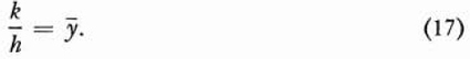
The general problem of finding the formula relating y and x when we are given ![]() as a function of x is handled by the method illustrated in our example of
as a function of x is handled by the method illustrated in our example of ![]() ; that is, we must examine the formulas whose rates of change we have previously determined and try to locate among these derivatives the rate of change we are concerned with. Since this rate of change has been previously derived from some formula relating y and x, that formula is the answer to our problem; in addition, we can add any constant to the formula and still have the correct answer. The process of searching among all formulas whose rates of change have previously been found may seem to be haphazard. But in practice mathematicians tabulate these formulas according to distinctive properties, so that a little experience with the tables usually enables one to find the desired formula. Since we are limiting the variety of formulas and their derivatives to a few cases, we shall not bother to become acquainted with a table. Instead we shall seek to recall the formulas and their derivatives which were calculated in the preceding Chapter.
; that is, we must examine the formulas whose rates of change we have previously determined and try to locate among these derivatives the rate of change we are concerned with. Since this rate of change has been previously derived from some formula relating y and x, that formula is the answer to our problem; in addition, we can add any constant to the formula and still have the correct answer. The process of searching among all formulas whose rates of change have previously been found may seem to be haphazard. But in practice mathematicians tabulate these formulas according to distinctive properties, so that a little experience with the tables usually enables one to find the desired formula. Since we are limiting the variety of formulas and their derivatives to a few cases, we shall not bother to become acquainted with a table. Instead we shall seek to recall the formulas and their derivatives which were calculated in the preceding Chapter.
For the following problems, find the formula which relates the variables whose instantaneous rate of change is given:
a) ![]() = 3x2
= 3x2
b) ![]() = 5
= 5
c) ![]() = x
= x
d) ![]() = 3x
= 3x
e) ![]() = 2t
= 2t
f) ![]() = 32t
= 32t
g) ![]() = 32
= 32
h) ![]() = 2t + 10
= 2t + 10
i) ![]() = −32t + 128
= −32t + 128
j) ![]() = −32
= −32
k) ![]() = 32t
= 32t
We shall now present some examples of the usefulness of integration in physical problems. Galileo had found that all objects falling to earth from points near the surface of the earth possess the same acceleration, namely 32 ft/sec2. This acceleration is constant; that is, it is the same at each instant of the fall. Now the acceleration at any one instant is the instantaneous rate of change of velocity with respect to time. Hence, instead of writing a = 32, we can equally well write
The physically important question is, What formula relates v and t? By reviewing the formulas for which we obtained rates of change [see formula (20) of Chapter 16] we find that v = 32t + C, where C is any constant.
In a particular physical problem, the quantity C can be chosen to fit the situation. Thus suppose that the object is merely dropped to earth; that is, at the instant it begins to fall its velocity is zero. If time is measured from the instant the object begins to fall, then the velocity v at t = 0 is zero. Hence, to make the formula
fit the physical fact that v must be zero when t = 0, we must have
0 = 32 · 0 + C,
or C = 0. Hence
is the answer to this particular problem in which the object is dropped, and time is measured from the instant it begins to fall.
Physical problems often require knowledge of the distance which an object falls in time t. Since the instantaneous velocity is the rate of change of distance with respect to time, then if d denotes the distance the object falls, ![]() = v. In view of (3), which applies when an object is dropped, we may state that
= v. In view of (3), which applies when an object is dropped, we may state that
We now wish to find the formula which relates d and t. Again we appeal to our experience with formulas and their derivatives [see formula (15) of Chapter 16] and note that the formula d = 16t2 has the derivative given by (4). However, the formula:
where C is any constant, also has the derivative (4). Since we have no reason to ignore the constant, we must accept (5) as the formula for the distance fallen in time t. However, if we agree to measure the distance fallen from the point where the object happens to be at the instant it starts to fall, and if time of fall is also measured from this instant, then it follows that d = 0 when t = 0. Substituting these values in (5) yields
0 = 16 · 0 + C,
and we see that C must be zero if formula (5) is to represent our situation. Hence
gives the distance the dropped object falls in time t if time is measured from the instant the object begins to fall and if distance is measured from the point where the object is at t = 0.
We have been able to reverse or invert the process of finding the rate of change of a function and thus proceed from a knowledge of acceleration to velocity as given by (3), and from velocity to distance fallen as given by (6). Before we comment further, let us consider some other situations.
Suppose that an object is thrown downward and leaves the hand with a velocity of 100 ft/sec. The acceleration is still given by (1), and so the speed is still given by (2). However, if time is measured from the instant the object leaves the hand, then at the instant t = 0, v = 100. To make the formula
v = 32t + C
fit this new situation, we must have v = 100 at t = 0, or
100 = 32 · 0 + C,
or C = 100. Hence
is the final formula for the velocity of an object thrown downward with an initial speed of 100 ft/sec.
Now let us seek the distance covered in time t. We know that the instantaneous velocity is the instantaneous rate of change of distance with respect to time. Thus, if we denote distance by d, we may write d = v. In view of (7), we have
We must now ask, What formula relates d and t? By reviewing the derivatives and the functions from which they were obtained, we find that the term 32t in (8) must come from the term 16t2 and the term 100 must come from 100t. The formula for d therefore is presumably d = 16t2 + 100t. However, we must recall that the formula
where C is any constant, also has the derivative (8). Hence, so far (9) is the general formula for distance fallen. If we agree to measure distance from the point at which the object happens to be when it begins to fall, and if time is measured from the instant the object begins to fall, then d = 0 when t = 0. Substituting these values in (9), we have
0 = 16 · 0 + 100 · 0 + C,
whence C = 0, and
is the final formula for our situation.
We see from the examples already presented that the occurrence of the constant C in the integration is not a disadvantage but rather an advantage. It permits us to adjust the formulas for velocity and distance to the specific situation we wish to describe, although the basic fact in all instances is ![]() = 32.
= 32.
The applications of integration made thus far have involved proceeding from the constant acceleration of 32 ft/sec2 to the formula for distance. But this we were also able to do in Chapter 13 without depending upon the calculus. It might seem that, thus far at least, the process of integration has not added at all to the power of mathematics. However, there are two points to be taken into consideration. The derivation of formula (10), for example, from the basic physical fact, a = 32, is much more readily done by integration than by the argument given in Chapter 13. But the second and more important point is that the method displayed here for the derivation of the formula for velocity from that for acceleration and of the formula for distance from that for velocity applies to all formulas, whereas the argument given in Chapter 13 is limited to constant acceleration. Thus, if an object should move with variable acceleration, as is the case when an object falls to the earth from a great height, then the method of Chapter 13 no longer applies, whereas integration does. We shall treat such problems later.
Since the motions of objects thrown up into the air are very important, let us note that our present method applies to them also except for minor modifications. We shall again restrict ourselves to objects which do not rise very far from the surface of the earth, so that we can continue to use the physical fact that the acceleration is constant and equal to 32 ft/sec2. When we studied the motion of a freely falling object, we decided, for convenience, to consider the acceleration to be positive. As a consequence, the velocity at any instant of time and the distance fallen turned out to be positive. However, an object thrown up into the air will, of course, rise and then fall. Hence, if we regard the velocity in the upward direction to be positive, then we must take the acceleration to be negative because it causes speed in the downward direction. We start then with the basic fact that
By integration we obtain
To fit the value of C to our situation, we shall use the physical fact that at t = 0, that is, at the instant at which the object is thrown upward, the hand or possibly a gun imparts to the object a velocity of, say 100 ft/sec, Thus at t = 0, v = 100. If we substitute these values in (12), we have
100 = –32 · 0 + C.
Hence C = 100, and the final formula for velocity is
Since, as we know, instantaneous velocity is the instantaneous rate of change of distance with respect to time, we can now apply integration to find the distance traveled. Let us use d to represent the height above the ground reached by the object in time t. Then by integrating (13) we obtain [cf. (9)]
We now wish to adjust the value of C to fit the physical situation. At the instant t = 0, the object is about to be thrown up, and at this instant, d = 0. If we substitute 0 for d and 0 for t in (14), we obtain
0 = –16 · 0 + 100 · 0 + C,
and so C = 0. Thus the final formula for height above ground is
Having obtained various formulas for velocity and distance such as (13) and (15) or (7) and (10), we can now proceed to solve problems of the type considered in Chapter 13. We shall not repeat this work here, but instead propose to show in the following sections how integration, or the inverse of differentiation, produces useful formulas from basic physical facts.
In all of the following problems the motions involved take place near the surface of the earth. Hence you may assume that the acceleration is constant.
1. Suppose that an object is thrown up into the air with an initial velocity of 150 ft/sec. Derive the formulas for the velocity and height above the ground.
2. Given that an object is dropped and falls to earth. Suppose that distance is measured from a point 50 ft above the point at which the object is dropped, but that time is measured from the instant the object begins to fall. What formula relates distance fallen and time of fall?
3. Suppose that an object is dropped from a point 75 ft above the ground. Derive the formulas for the velocity and height above the ground.
4. Suppose that an object is thrown up into the air from the roof of a building 50 ft high. The initial velocity is 100 ft/sec. Derive the formulas for the velocity and for the height above the ground.
5. Suppose an object is thrown downward from the roof of a building 50 ft high and that the initial velocity is 100 ft/sec. Derive the formulas for the speed and height above the ground.
The derivation of formulas useful in the study of motion was one of the seventeenth-century problems which motivated the creation of the calculus. Another basic class of problems was concerned with finding the lengths of curves, the areas bounded by curves, and the volumes bounded by surfaces. In Section 16–2 of the preceding chapter, we mentioned a few problems which called for the determination of lengths, areas, and volumes. The expansion of science and technology has brought about literally thousands of new uses of curves and surfaces for which the very same quantities are required. The distance a ship travels along the spherical surface of the earth is the length of a curve. Cables and roadways of bridges are curves, and in planning the construction one must know the lengths of these cables and roadways. The weights of various objects employed in scientific and engineering projects are easily obtained once the volumes are known. For example, if a steel beam of some particular shape is to be used in the framework of a building, then, since the material is the same throughout the beam, the weight is merely the volume multiplied by the weight per cubic foot of the metal. Hence volume is the essential quantity to be determined.
But problems concerning lengths of curves, areas, and volumes had already been solved in Euclidean geometry. Why should they then have presented special difficulties to the scientists of the seventeenth century? The answer is that Euclidean geometry is adequate only to treat figures bounded by straight line segments and by circles. This limitation is inherent in the subject. Examination of the axioms of Euclidean geometry shows that they state properties of lines and circles. Naturally the theorems which can be deduced readily must also be limited to such figures. Although the Greeks managed to compute a few areas and volumes of figures bounded by other geometrical shapes, they were able to do so only with great difficulty and by introducing special methods limited to the figures in question. The variety and number of problems which arose in the seventeenth century demanded more general and more easily applicable methods.
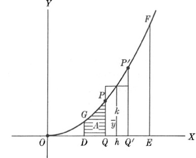
Fig. 17–1.
The area under the curve is that swept out by the vertical line QP as it moves to the right.
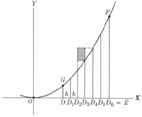
Though it is by no means evident, the calculus proves to be the very mathematical tool which enables us to calculate the lengths of curves, the areas bounded by curves, and the volumes bounded by surfaces. We shall illustrate this fact by treating the problem of area. Let us try to determine the area DEFG of Fig. 17–1. This area is bounded by the vertical line segments DG and EF, by the segment DE and by the arc FG of the curve whose equation is, say y = x2. We may think of this area as being swept out by a vertical line segment PQ which starts at the position DG and moves to the right. Naturally the length of PQ varies as it moves. Let us suppose that PQ has reached the position shown in the figure. The area swept out by this moving segment depends, of course, upon the position it has reached. This position can be specified by the x- value of the point Q. Hence the variable area, which we shall denote by A, is a function of x, the abscissa of the point Q. We now propose to find the formula which relates A and x. Our procedure is as follows: We begin by determining the rate of change of A with respect to x at any given x and integrate this derivative to arrive at the desired formula.
Our first task therefore is to find the rate of change of A with respect to x.* To do so, let us suppose that PQ has moved a little farther to the position P′Q′. The abscissa of Q′ is, of course, somewhat larger than that of Q. Let us denote the abscissa of Q′ by x + h, so that the increase in the abscissa from Q to Q′ is h. Obviously, the variable area A also increases when PQ moves to P′Q′. Let us use k to denote this increase which geometrically is the area QQ′P′P. It is immediately evident that the increase is equal to the area of a rectangle whose base is h and whose height is an ordinate, ![]() , which is larger than PQ and smaller than P′Q′.(We do not know how large
, which is larger than PQ and smaller than P′Q′.(We do not know how large ![]() is, but we shall see in a moment that this does not matter.) We have, then,
is, but we shall see in a moment that this does not matter.) We have, then,
Let us divide both sides of (16) by h. Then
Now k/h is the average rate of change of area with respect to the abscissa in the interval h. By the very definition of an instantaneous rate, the rate of change of area with respect to abscissa at the x-value of Q should be the limit of the average rate of change as h approaches zero. But as h approaches zero, ![]() approaches the y-value of P, or the length PQ. Thus
approaches the y-value of P, or the length PQ. Thus
Since the y in (18) is the ordinate of the point P and P lies on the curve OGF, it follows that y = x2. Then
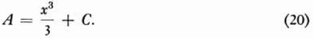
We now have the rate of change, with respect to x, of the variable area A. To find A itself, we must ask ourselves what formula has the derivative x2. A review of previously obtained derivatives tells us that the derivative of x2 is 3x2, and that therefore A = x3/3. We know, however, that the integral may contain a constant term and that this will not affect the derivative, which will remain unchanged. Hence the full answer is:
To determine the value of C, we make use of the fact that when PQ is at DG, the area is zero because DG was the starting position of PQ. Suppose that the x-value of D is 3. Then, by substituting 0 for A and 3 for x in (20) we have
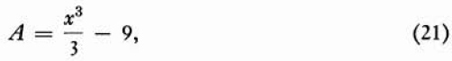
or C = –9. Thus
and this formula gives the area between DG and the variable position of the moving line segment PQ. If we wish to determine the area from DG to EF, we may assume that PQ has reached the position EF. Let us suppose that the x-value of E is 6. If we now substitute 6 for x in (21), we obtain the area DEFG. Hence
Thus we have found the area bounded by a curve through the process of integration. We have, of course, used the equation of the curve, which, thanks to Descartes and Fermat, should be known to us.
In working problems, one can eliminate some writing by neglecting to introduce the constant C in (20) and using just the formula A = x2/3. We then substitute 6, which is the abscissa of the point E, in this formula; next, we substitute 3, which is the abscissa of the point D; and finally we subtract the second result from the first. These steps lead to the result given by (22).
1. Find the area bounded by the curve y = x2, the X-axis, and the ordinates at x = 2 and x = 6.
2. Find the area bounded by the curve y = x2, the X-axis, and the ordinates at x = 4 and x = 6.
3. Find the area bounded by the straight line y = x, the X-axis, and the ordinates at x = 4 and x = 6.
4. Find the area bounded by the curve y = x2 + 9, the X-axis, and the ordinates at x = 3 and x = 6.
An important quantity for scientific and engineering purposes is the work done in various physical operations. When a person raises an object for some distance he does work. The definition of the word “work” as used in the physical sciences is the product of the force applied and the distance through which the force acts. This quantity is important, for example, in the operation of machinery. One must know how much work a machine is capable of doing, to decide whether it is suitable for a particular task. A train pulling a load over some distance and an airplane carrying freight or passengers do work, and again the capacity of these carriers and the fuel requirements must be known for proper design.
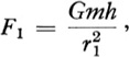
We shall now consider how the calculus can be used to calculate work. Let us suppose that we wish to compute the work required to raise a 500-pound load to a height of 100 miles. This problem arises, for example, in determining the quantity of fuel required to raise a rocket to some desired height. Now the force that will accomplish this goal must be great enough to offset the force of gravity, which pulls the object down. The force of gravity, as we know, is given by
where G is the gravitational constant, M is the mass of the earth, m is the mass of the object, and r is the variable distance between the position of the object and the center of the earth. In our problem, we shall regard G, M, and m as constant, so that the only variables in (23) are F and r.(However, in actual rocket problems, the fuel itself is part of the load which must be raised, and, since the fuel is gradually burned up as the rocket rises, the mass m also is a variable.) Since the object is to travel a distance of 100 miles up, the force which must be applied varies over the distance. Hence it is not possible to calculate the work by merely multiplying the force by the distance.
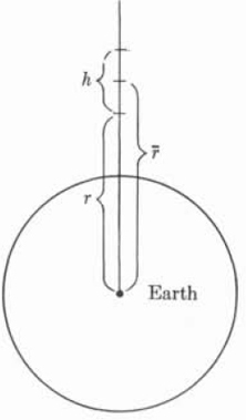
Let W be the work required to raise the object from the surface to some distance r from the center of the earth. Of course, W is a function of r and is unknown. Let us suppose that the object is raised an additional distance h, that is, from r to r + h (Fig. 17–2). The corresponding extra work, k, again depends upon the force which must be applied [given by (23)] and the distance, h, over which it operates. However, the force varies even as r increases to r + h. Let ![]() be some value of r between r and r + h such that the corresponding force
be some value of r between r and r + h such that the corresponding force ![]() is the average force required during the interval r to r + h. This last-mentioned force is entirely analogous to the quantity
is the average force required during the interval r to r + h. This last-mentioned force is entirely analogous to the quantity ![]() introduced in the treatment of area as an average ordinate in the interval h on the X-axis. We shall see in a moment that the precise value of
introduced in the treatment of area as an average ordinate in the interval h on the X-axis. We shall see in a moment that the precise value of ![]() plays no role.
plays no role.
Fig. 17–2
Then the work done in raising the mass m from r to r + h is
Equation (24) yields the additional work required to raise the object the distance h. We shall determine next the average rate of change of work with respect to distance. This quantity, k/h, is obtained from equation (24) by dividing both sides by h. Thus
We compute next the instantaneous rate of change of work with respect to distance. This rate is obtained by letting h approach zero and finding the limit approached by k/h. However as h approaches zero, the quantity ![]() must approach r because
must approach r because ![]() is always intermediate between r and r + h. Then the instantaneous rate of change of work with respect to distance is given by
is always intermediate between r and r + h. Then the instantaneous rate of change of work with respect to distance is given by
Since we now know ![]() , we can find W by integration; that is, we examine the various functions we have differentiated, to find one which yields (25) as its derivative. It so happens that in our work we did not encounter the rate of change given by (25), but we can take for granted now and check later that the function corresponding to this derivative is
, we can find W by integration; that is, we examine the various functions we have differentiated, to find one which yields (25) as its derivative. It so happens that in our work we did not encounter the rate of change given by (25), but we can take for granted now and check later that the function corresponding to this derivative is
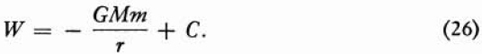
To determine the constant of integration, we recall that when r = 4000 miles or 4000 · 5280 feet, the object is on the surface of the earth, and hence, W = 0. Since we do not wish to manipulate large numbers at the moment, we denote the radius of the earth by R. Then when r = R, W = 0. We substitute these values in (26) and obtain
or
Hence
We now have the function which expresses the work done in raising an object of mass m from the surface of the earth to a height r units from the center. By substituting the numerical data at our disposal we can calculate the work done in the example proposed at the outset. We know G and the mass M of the earth. The quantity R is 4000 · 5280 feet, and the value of r is 4100 miles or 4100 · 5280 feet. The mass m, in our example, is the mass of an object which weighs 500 pounds or 500–32 poundals at the surface of the earth. Hence the mass m is 500 pounds.
We can simplify the arithmetic somewhat since we know that the acceleration due to the earth’s gravitational attraction is [formula (5) of Chapter 15]
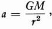
and that when r = R, then
a = 32 ft/sec2.
Thus
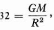
whence
GM = 32R2.
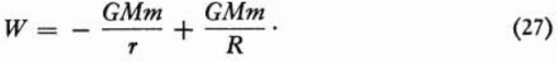
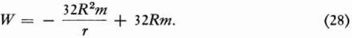
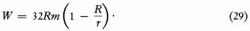
If we substitute this result in (27), we obtain
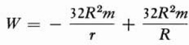
or
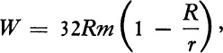
By applying the distributive axiom we may write
Formula (29) is the useful form for the calculation of the work, except for one detail. The unit of work is usually taken to be foot-pounds. However if the mass m is given in pounds, then the formulas we have employed here and elsewhere express the force in poundals. Hence formula (29) yields the work done in foot-poundals. To obtain an answer in foot-pounds we just ignore the factor 32 in (29).
1. Calculate the work done in raising the 500-lb weight to a height of 100 mi.
2. Suppose that one neglected the variation in gravitational force with height and assumed that the 500-lb weight remains constant over the 100 mi that it is raised. What is the work required to raise it?
3. A cable weighing 2 lb/ft is suspended in a well 100 ft deep; a tool weighing 300 lb is attached at the cable’s lower end. Find the work done to raise the tool to the surface. [Suggestion: Let W be the work done to raise the tool x ft. Since now only 100 − x ft of cable remain, the work k done in raising the tool h feet more is k = [300 + 2(100 − ![]() )]h, where
)]h, where ![]() is some value of x between x and x + h. Now find
is some value of x between x and x + h. Now find ![]() , and then W. Determine the constant and compute the work done.]
, and then W. Determine the constant and compute the work done.]
4. Use the method of increments to show that the function W = c/r, where c is any constant, has the derivative ![]() .
.
We can use the theory of the preceding section to answer a question which is of special interest today, namely, what velocity one must give to a rocket to ensure that it just reaches a specified height. The condition intended here is that the rocket will have zero velocity when it reaches this height, for if it still possessed some velocity, it would continue to rise.
As the rocket travels upward, it loses velocity because the acceleration of gravity, which is directed downward, continually decreases the velocity. However, if the initial velocity V is properly chosen then the rocket will have zero velocity at the required height. We wish to determine V.
In the preceding section we calculated the work done in raising an object to a height of d feet above the surface of the earth. However the result did not involve the initial velocity V. We shall therefore obtain another expression for this work. It is physically clear that the work done against gravity in the process of sending an object up with some initial velocity V to reach a height of d feet should equal the work done by gravity acting on the object when it falls d feet. Hence let us calculate the latter. We have an object which begins its fall with zero velocity and falls d feet. Since it gains velocity on the way down in just the reverse order in which it loses velocity on the way up, it strikes the ground with a velocity of V ft/sec.
If an object falls from a great height above the surface of the earth, it does not fall with constant acceleration. However, there is some average acceleration which would produce the same final velocity in any time of fall. Let us denote this average acceleration by a. In Section 13–5 we found the formula for the speed of and the distance fallen by an object which is dropped and falls to earth with an acceleration of 32 ft/sec2. If the acceleration were a instead of 32, the formulas would be (Exercise 14 of Section 13–5)
![]()
Now, if we take the value of t from the first formula and substitute it in the second one, we obtain the relationship between d and v. Thus since t = v/a,
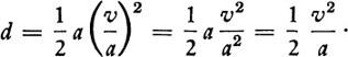
Then
wherein we have written V merely to denote that it is the final velocity after the object has fallen d feet.
Since the object falls with a constant acceleration a, the force which gravity applies, by Newton’s second law of motion, is ma, where m is the mass of the rocket. Then the work done by gravity is
W = mad.
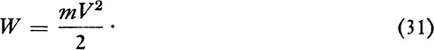
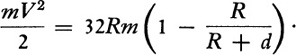
However by (30) we see that ad = V2/2. If we substitute this value in the formula for W we have
Formula (31), then, is an expression for the work that gravity does in causing an object to fall a distance d and to acquire, at the end of the fall, the velocity V. As we have already noted, this is the work we must do to raise the object from the surface of the earth where it has velocity V to the point where it has velocity zero.
Formula (29), namely,
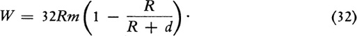
also gives the work required to raise an object from the surface of the earth to the distance r from the center. Let r = R + d so that the object is raised to the height d above the surface. Then
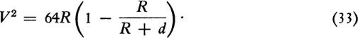
We now have two expressions, formulas (31) and (32), for the work. We equate them and obtain
Dividing both sides by m and multiplying by 2 yield
This then is the expression for the initial velocity required to send an object up so that it just reaches the height of d feet above the surface. In applications, the quantities occurring in formula (33) must be expressed in feet.
Formula (33) has a very interesting consequence. If we wished to send an object farther and farther up so that d becomes indefinitely large, then, since R is fixed, the quantity R/R + d approaches zero. The result is
V2 = 64R
or
This velocity is often described as the velocity required to reach infinity and is called the escape velocity. Of course, infinity is not a geographical location, and what is really meant is that the object will keep going out indefinitely and never return. If the initial velocity is less than the escape velocity, then the object will attain zero velocity at some finite, though possibly large, distance from the earth and fall back to earth.
We can readily calculate the escape velocity. Since
R = 4000 · 5280 = 21,120,000 ft,
we have
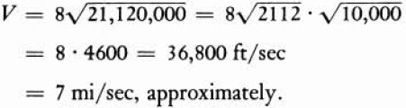
This is the velocity necessary to escape from our trouble-infested earth.
1. Calculate the velocity required to send an object 240,000 mi up (this is the distance to the moon) and arrive there with zero velocity. [Suggestion: Use (33).]
2. Does formula (34) give the escape velocity from the moon, that is, does it give the velocity required to send an object from the moon to infinity? If not, how should it be modified?
In our discussion of integration as a means of finding areas bounded by curves, we mentioned that from Greek times up to the seventeenth century the efforts of mathematicians to determine such areas had not been very successful. The reason, already noted, was that these men tried to use Euclidean geometry, and this geometry is limited in power. To prove theorems about the areas of figures bounded by curves, they had to overcome great difficulties by a special method known as the method of exhaustion. They approximated the area in question by figures bounded by straight lines—for such figures the area could readily be found—and then considered what happened as the approximation was improved more and more. Although, for the moment, it may seem that we are taking a step backward, we shall nevertheless reapproach the problem of area by adopting the Greek view. We shall find that our reexamination will have fruitful results for a new and wide class of problems.
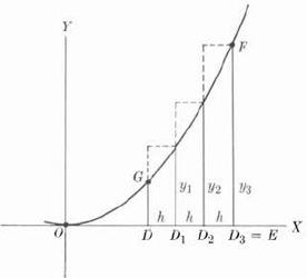
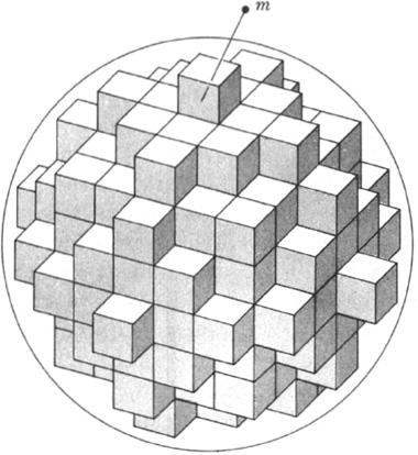
Let us consider the problem [treated in Section 17−4] of finding the area DEFG (Fig. 17–3) which is bounded by the arc FG of the curve whose equation is y = x2, by DE, and by the vertical line segments DG and EF. We subdivide the interval DE into three equal parts, each of length h, and denote the points of subdivision by D1, D2, and D3, where D3 is the point E. Let y1, y 2, and y3 be the ordinates at the points of subdivision. Now y1h, y2h, and y3h are the areas of three rectangles shown in Fig. 17–3, and the sum
is the sum of the three rectangular areas and thus an approximation to the area DEFG.
Fig. 17–3.
The area under a curve approximated by a sum of rectangular areas.
Fig. 17–4.
Decreasing the widths of the rectangles improves the approximation provided by the sum of the rectangular areas.
We can obtain a better approximation to the area DEFG by using smaller rectangles and more of them. To illustrate this point, suppose that we subdivide the interval DE into six parts. Figure 17−4 shows what happens to the middle rectangle of Fig. 17–3. This rectangle is replaced by two, and because we use the y-value of each point of subdivision as the height of a rectangle, the shaded area in Fig. 17–4 is no longer a part of the sum of the areas of the six rectangles which now approximates the area DEFG. Therefore the sum
is a better approximation to the area DEFG than the sum (35).
We can make a more general statement concerning this process of approximation. Suppose that we divide the interval DE into n parts. There would then be n rectangles, each of width h. The ordinates at the points of subdivision are y1, y2, . . . , yn, where the dots indicate that all intervening y-values at points of subdivision are included. The sum of the areas of the n rectangles is then
and the dots again indicate that all intervening rectangles are included. In view of what we said above about the effect of subdividing DE into smaller intervals, the approximation to the area DEFG given by the sum (37) improves as n increases. Of course, as n gets larger, h gets smaller because h = DE/n.
We see so far how figures formed by line segments—rectangles in the present case—can be used to provide better and better approximations to an area bounded by a curve. Thus far we have utilized the Greek idea. We now depart from it somewhat and introduce the concept of a limit. Specifically the area DEFG is the limit approached by the sum of the rectangles as the number of rectangles becomes larger and larger, or, one says, as the number of rectangles becomes infinite. Thus the number of rectangles might be successively 3, 6, 12, 24, 48, . . . , where the dots indicate that we continue to double the number indefinitely. Of course, h, the width of each rectangle, approaches zero. In symbols, we write
the symbol ![]() means that what we wish to obtain is the number approached by the sum in parentheses as h approaches zero.
means that what we wish to obtain is the number approached by the sum in parentheses as h approaches zero.
What have we accomplished? We seem to have made a simple thing difficult. The innocent area DEFG has been approximated by a sum of rectangles and, as the number of rectangles increases (while each rectangle becomes thinner), the sum becomes a better and better approximation of the area DEFG. However, we know from Section 17−4 that the area DEFG may be obtained in the following way: If the equation of the curve FG is y = x2, we find the formula whose derivative is x2 or, in other words, we find the integral of x2. This happens to be x3/3. We substitute the abscissa of the point E and obtain a number. We next substitute the abscissa of the point D and obtain a number. Finally, we subtract the latter result from the former. We see, then, that limits of the kind expressed in (38) can be determined by integration and the subsequent numerical work just described.
Now insofar as obtaining areas is concerned, we do not seem to have accomplished very much. Actually, were we to pursue the subject of area a little further than we shall in this book, we would find the new point of view significant in this very connection. However, we shall go on to other applications in which the fact that a limit of the form (38) can be obtained by integration will be the key to the solution.
It is helpful to shorten the writing of an expression such as (38). The notation used in calculus books is
This notation must not be taken too literally. The symbol ʃ is an abbreviated S and is intended to denote that we are dealing with the limit of a sum. For areas this sum is a sum of rectangles. The y in (39) indicates that the heights of these rectangles are ordinates of some curve, and the dx indicates that the base of each rectangle is a small interval along the X-axis. The number a is the abscissa of the left-hand end point of the interval DE, and the number b is the abscissa of the right-hand end point. The entire expression on the right side of (39) is called the definite integral of the function represented by y. The words “definite integral” denote that we are interested in the integral regarded as the limit of a sum.
Whereas Newton had concentrated on finding the derivatives of given functions and on the inverse process, the recognition that limits of sums, such as that expressed by (38), can be obtained by reversing differentiation is due primarily to Gottfried Wilhelm Leibniz (1646−1716). Leibniz’s career contrasts sharply with Newton’s. Newton, as we know, had undertaken the study of mathematics and physics early in life and had pursued these two fields almost exclusively, although he did make minor contributions to chemistry and theology. His career as a professor gave him the opportunity to concentrate. Leibniz started by studying law at the University of Leipzig, the city in which he was born and lived as a youth. He secured a bachelor’s degree at Leipzig and in 1666 a doctor’s degree at the University of Altdorf. His first position was that of ambassador for the Elector of Mainz, and until 1672 his interest in mathematics was secondary. In 1672, during a trip to Paris on behalf of his employer, he met Huygens, who acquainted Leibniz with current scientific problems and activities. Leibniz’s interests were deeply stirred and thereafter he devoted much time to mathematics. In 1676 he was appointed librarian and councillor to the Elector of Hannover and, although this position also entailed many administrative duties, he nevertheless had more leisure for academic pursuits. In 1700 he went to Berlin to work for the Elector of Brandenburg and, while there, founded the Berlin Academy of Sciences. What is amazing about the man is the vast quantity of first-rate contributions’ to many fields. Although his profession was jurisprudence, his work in mathematics and philosophy ranks among the best the world has produced. He also did major work in mechanics, nautical science, optics, hydrostatics, logic, philology, and geology, and was a pioneer in historical research. Throughout his life he tried to reconcile the Protestant and Catholic faiths. We may recall also his previously noted activities—his efforts to organize a society devoted to the dissemination of the new scientific knowledge and to turn the German language into a suitable vehicle for the new ideas. No subject pursued by intellectuals of his age was neglected; only Leibniz himself went unrecognized and neglected by his contemporaries.
From our present point of view, Leibniz’s emphasis on area as a limit of a sum may seem to be no blessing. But the full import of what he taught, namely that such limits can be evaluated by reversing differentiation, is of vast significance because limits of sums arise naturally in physical problems. Let us consider an example. In Newton’s and Leibniz’s time and for one hundred years thereafter, one of the major problems was to calculate the gravitational force exerted by one mass on another. If these masses are so compact that they can be regarded as concentrated at points, then the distance between them is the definite distance between these points, and the force of attraction is given by the usual formula. If, however, one mass is the earth and the other is some small object at, say a distance of a few hundred miles from the earth, then, although the latter may in many cases be considered as concentrated at a point, the earth itself cannot be so regarded. The difficulty is that the mass of the earth is distributed over an enormous volume and hence cannot be said to be separated from the mass m by a definite distance.
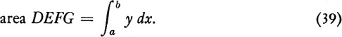
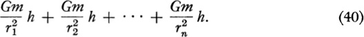
We can, however, regard the volume of the earth (Fig. 17–5) as broken up into small cubes numbered from 1 to n.* Since each cube is small, a good approximation of the distance of a cube from the mass m is the distance from the center of the cube to the mass m. Thus if this distance is r1 for the first cube, then the gravitational attraction exerted by the cube on the mass m is given by
Fig. 17–5.
The volume of sphere approximated by a sum of cubical volumes.
where h now stands for the mass of the cube. The same applies to each cube up to the nth. cube. Then the total gravitational attraction F of the n cubes is
Formula (40) is entirely analogous to (37). The quantity y1 in (37) has now become ![]() ; y2 has become
; y2 has become ![]() ; and so forth. But (40) is not the exact expression for the attraction exerted by the earth because it assumes that each cube acts as though its mass were concentrated at its center. However, if we make each cube smaller, which means that h will be smaller, and increase the number of cubes, n, so that they continue to fill as much of the sphere as possible, the sum of attractions exerted by the n cubes will be a better approximation to the force of attraction exerted by the entire sphere. The reason is that the smaller the cube, the more appropriate it is to assume that its mass can be regarded as concentrated at its center. The exact value of F is
; and so forth. But (40) is not the exact expression for the attraction exerted by the earth because it assumes that each cube acts as though its mass were concentrated at its center. However, if we make each cube smaller, which means that h will be smaller, and increase the number of cubes, n, so that they continue to fill as much of the sphere as possible, the sum of attractions exerted by the n cubes will be a better approximation to the force of attraction exerted by the entire sphere. The reason is that the smaller the cube, the more appropriate it is to assume that its mass can be regarded as concentrated at its center. The exact value of F is
Formula (41) is exactly like (38). It is now clear that to determine the total gravitational attraction exerted by a distributed mass, the earth in our discussion, we must calculate the limit of a sum. We know that such limits can be calculated by reversing differentiation. The particular limit in (41) cannot be computed with the mathematics at our disposal. The reason is that h in (41) is three-dimensional (because it is mass per cubic foot times volume), whereas the h in (38) is a segment. Hence (41) is a little more complicated than (38). But our example makes the point that limits of sums arise in physical problems, and that we can evaluate them by reversing differentiation.
As a matter of history, Newton solved the very problem we have been considering and proved that the earth attracts a small mass as if the entire mass of the earth were concentrated at its center. In other words, although the earth’s mass is distributed over a large region, it happens to be true that a spherical mass attracting a small mass can be treated as if its mass were concentrated at its center. The solution of this problem enabled Newton to make further advances in the theory of gravitation. In our discussion of the law of gravitation, we also considered the quantity r to be measured from the center of the earth; that is, we made implicit use of Newton’s result.
We could continue to study extensions and further applications of the calculus, but there are other features of this mathematical development which take precedence in view of the time we can devote to the subject. In the first place, it is most important to note that the calculus rests on a new concept, the concept of the limit of a function. We employed this concept in two essential ways. In the differential calculus we introduced the instantaneous rate of change of a function. This rate is the limit of the average rate of change of speed, that is of k/h, as h approaches zero. In the integral calculus we used the limit concept to speak of the quantity approached by the sum
y1h + y2h + · · · + ynh
as h approaches zero. This limit can represent aroa, the gravitational force exerted by an extended body, or other quantities, depending upon the physical or geometrical interpretation of the function relating y and x, and of h. Thus it is this new concept which distinguishes the calculus from the branches of mathematics previously studied.
The limit was defined as the number approached by some function of h as h approaches zero. This description is admittedly vague. In particular, the word “approach” is suspect. If for smaller and smaller values of h the ratio k/h should have the values ![]() ,
, ![]() ,
, ![]() ,
, ![]() , . . . , are these values approaching 1? They are, in the sense of getting closer to
, . . . , are these values approaching 1? They are, in the sense of getting closer to ![]() , but it is also clear that they are always less than, and so the limit might very well be
, but it is also clear that they are always less than, and so the limit might very well be ![]() . In other words, how closely must the values of k/h approach a particular number before we can decide that that number is the limit of k/h? We shall not attempt to give a precise formulation of the limit concept. However, it may be a comfort to know that a precise definition can be given today.
. In other words, how closely must the values of k/h approach a particular number before we can decide that that number is the limit of k/h? We shall not attempt to give a precise formulation of the limit concept. However, it may be a comfort to know that a precise definition can be given today.
The history of the efforts of mathematicians to grasp this concept properly is instructive as to how mathematics develops. The trouble started early in the seventeenth century. We have already mentioned that many mathematicians of that century made contributions to the calculus, even before Newton and Leibniz began to work on the subject. These forerunners realized that they were unable to give satisfactory expositions of their ideas and, in fact, hardly comprehended the significance of what they were creating. Despite the long tradition of rigorous proof in mathematics, the early workers in the calculus did not hesitate to advance their crude and imprecise ideas and defended themselves in ways that seem strange for mathematicians. Rigor, said Bonaventura Cavalieri, a pupil of Galileo and professor at the University of Bologna, is the concern of philosophy and not of geometry. Pascal argued that the heart intervenes to assure us of the correctness of mathematical steps. Proper finesse rather than logic is what is needed to do the correct thing, just as, he added, the appreciation of religious grace is above reason.
Although Newton and Leibniz made the most significant advances in the formulation of the ideas and methods of the calculus, neither contributed much to the rigorous establishment of the subject. They both realized that they had not presented clearly and precisely the basic ideas of instantaneous rate of change and the definite integral. Yet they were sure that their ideas were sound because they made sense physically and intuitively, and because the methods gave results which agreed with observations and experiments. Both gave many versions in the attempt to hit upon the precise concepts, but neither was successful. In some writings Leibniz went so far as to say that the methods of the calculus were only approximate, but since its errors were smaller than observational or measurable errors, the subject was useful.
The work of Newton and Leibniz was criticized even by their contemporaries. Newton did not reply to the criticisms, but Leibniz did. In addition to defending the methods by an appeal to the agreement of the results with experience, he attacked the critics as overprecise—a strange stand for a mathematician. He also said that we should not lose the fruits of an invention by excessive scruples. Of course, such replies did not provide the missing clarity and rigor. Some writers on the calculus proceeded as though there were no difficulties. Their attitude seemed to be that what was incomprehensible needed no further explanation.
The successors of Newton and Leibniz attempted to supply better foundations for the calculus. However their efforts were blocked in two ways. First of all, the formulations presented by Newton and Leibniz were different, but both yielded correct results; hence the rigorous construction of the calculus had to reconcile the two formulations. Secondly, the whole situation became complicated by an argument between Newton and Leibniz on the question of whether Leibniz had stolen ideas from Newton. Newton’s friends, and English mathematicians in general, sided with him, while continental mathematicians defended Leibniz. The quarrel between the two groups became so bitter that they stopped corresponding with each other for about one hundred years. English mathematicians continued to talk about fluents and fluxions, Newton’s terms for functions and their derivatives, whereas continental scientists talked about infinitesimals, Leibniz’s name for h and k or, in his notation, dx and dy.
Two of the greatest mathematicians of the eighteenth century, Leonhard Euler and Joseph Louis Lagrange, worked on the problem of clarifying the calculus, but without success. Both arrived at the conclusion that as it stood, the calculus was unsound, but that somehow errors were offsetting one another so that the results were correct. A more drastic opinion was offered by the mathematician Michel Rolle (1652–1719). He taught that the calculus was a collection of ingenious fallacies. Voltaire called the calculus “the art of numbering and measuring exactly a Thing whose existence cannot be conceived.” Near the end of the eighteenth century the distinguished mathematician Jean le Rond d’Alembert (1717–1783) felt obliged to advise his students that they should persist in their study of the calculus; faith would eventually come to them. All eighteenth-century attempts to supply rigorous foundations for the calculus failed. In the first quarter of the nineteenth century, Augustin-Louis Cauchy (1789–1857), the leading French mathematician, gave the first satisfactory definitions of the derivative and definite integral. Gradually other concepts of the calculus, which we have not considered, were clarified. The differences in notation were also eliminated.
This history of the development of the calculus is significant because it illustrates the way in which mathematics progresses. Ideas are first grasped intuitively and extensively explored before they become fully clarified and precisely formulated even in the minds of the best mathematicians. Gradually the ideas are refined and given the polish and rigor which one encounters in textbook presentations. In the instance of the calculus, mathematicians recognized the crudeness of their ideas and some even doubted the soundness of the concepts. Yet they not only applied them to physical problems, but used the calculus to evolve new branches of mathematics, differential equations, differential geometry, the calculus of variations, and others. They had the confidence to proceed so far along uncertain ground because their methods yielded correct physical results. Indeed, it is fortunate that mathematics and physics were so intimately related in the seventeenth and eighteenth centuries—so much so that they were hardly distinguishable—for the physical strength supported the weak logic of mathematics. Of course, mathematicians were selling their birthright, the surety of results obtained by strict deductive reasoning from sound foundations, for the sake of scientific progress, but it is understandable that the mathematicians succumbed to the lure.
It may be clear from this account of the difficulties that mathematicians experienced with the concept of limit that the two chapters devoted to the calculus do not provide a complete description of the concept and all its ramifications. The reader may justifiably feel some vagueness and uneasiness about what has been presented. Further study of the calculus would eliminate these objections. We must also point out that in illustrating the ideas of the calculus we have confined ourselves to the simplest functions. The subject is a vast one and far more powerful than we can indicate with the technique employed here. Indeed an enormous number of new branches of mathematics rest on the calculus. All of these, together with the calculus, constitute a division of mathematics, called analysis, which is considerably more extensive than algebra or geometry. But some glimpse of this most significant mathematical creation of modern times may in itself afford a rich enough reward.
1. What essentially new idea does the calculus treat?
2. Mathematicians are logical thinkers; they reason directly and flawlessly to the desired conclusions. Discuss this assertion in the light of the history of the calculus.
The men of the Renaissance had turned to new sources of knowledge—nature, reason, and mathematics—but were rather vague as to the specific methods by which they were to reconstruct the various branches of thought. Fortunately, a series of developments and creations not only gave strong impetus to the urge to rebuild knowledge, but actually supplied the method by which positive truths were to be attained. Galileo formulated this method clearly and applied it to obtain the laws of motion of objects moving on and near the surface of the earth. Newton conclusively demonstrated the efficacy of Galileo’s method and supplied the doctrine which was to be the keystone in any new system of thought: All bodies in the universe were subject to one set of physical axioms, and their behavior could be deduced from these axioms. Nature was mathematically designed, and natural phenomena adhered strictly to universal mathematical laws which described the behavior of a speck of dust and of the most distant stars.
The intellectual leaders of the seventeenth and eighteenth centuries believed that they now had the tenets which vouchsafed a totally new outlook on the universe and which justified a reconstruction of all of mankind’s systems of thought, institutions, and way of life. The right foundation in the form of a mathematical-mechanical explanation was available. New ideas, always far more effective in determining the course of cultures than wars or political events, began to work their influence, and the growing use of books permitted the leaders to reach large groups of people.
The intellectuals were confident that reason, based on the new truths made manifest by the mathematical and scientific work of the seventeenth century and cleansed of the metaphysical and theological presuppositions of the medieval period, could rebuild philosophy, religion, literature, art, political thought, and economic life. They saw clearly that mathematics and science were offering not just a few theorems and isolated results, but a new approach to truths and a new interpretation of the universe. Thus thinking men were impelled to a sweeping reorganization of all knowledge and institutions.
The eighteenth century has been called the Age of Reason. It was not the first period of history in which reason played a dominant role, but it was the first in which the intellectual elite emboldened by some successes in physical science dared to apply reason to the reconstruction of an entire civilization. The spirit and outlook of the leaders are indicated by their reference to their own age as the Enlightenment.
We cannot examine in the text the new doctrines which the Age of Reason fashioned in the social sciences, humanities, and the arts. The reader who would like to pursue this subject will find several survey chapters in the books by the author listed in the Recommended Reading. Further references are given in those chapters.
1. Suppose an object is thrown up from the ground with an initial velocity of 200 ft/sec. Using 32 ft/sec2 as the downward acceleration of gravity,
a) find the formula for its height above the ground in t sec;
b) calculate the maximum height to which the object will rise;
c) find the velocity with which the object will hit the ground.
2. Suppose that an object is thrown upward from the roof of a building which is 100 ft high and is given an initial velocity of 200 ft/sec.
a) Find the formula for its height above the roof in t sec.
b) Find the formula for its height above the ground in t sec.
3. The acceleration which the moon’s gravity imparts to objects near the surface of the moon is 5.3 ft/sec2. Suppose an object is thrown up from the surface with an initial velocity of 200 ft/sec. Find
a) the formula for the height of the object after t sec,
b) the maximum height the object reaches.
c) Comparing the answers to Exercises 1(b) and 3(b) should show that the object reaches a greater maximum height on the moon. Can you explain in physical terms why this must be so?
4. a) Find the area bounded by the straight line y = 3x, the x-axis, and the ordinate at x = 4 by using the calculus method.
b) The figure described in part (a) is a triangle. Find its area by using the appropriate theorem of Euclidean geometry. Does your result agree with the answer to part (a)?
5. a) Find the area bounded by the straight line y = 2x + 7, the x-axis, and the ordinates at x = 4 and x = 6.
b) The figure described in part (a) is a trapezoid. According to a theorem of Euclidean geometry the area of a trapezoid is one-half the altitude times the sum of the bases. Calculate the area by this formula and see whether it checks with the answer to part (a).
6. Calculate the work required to raise an object whose mass is 200 lb from the surface of the earth to a height of 100 mi. The variation in the earth’s gravitational force must be taken into account.
7. Suppose you wish to shoot a rocket up from the surface of the earth to a height of precisely 100 mi. What initial velocity must you give the rocket?
1. The predecessors of Newton and Leibniz in the creation of the calculus.
2. The work of Newton on the calculus.
3. The controversy between Newton and Leibniz on priority in founding the calculus.
BALL, W. W. ROUSE: A Short Account of the History of Mathematics, Chaps. 16 and 17, Dover Publications, Inc., New York, 1960.
BELL, ERIC T.: Men of Mathematics, Chap. 7, Simon and Schuster, Inc., New York, 1937.
COLERUS, EGMONT: From Simple Numbers to the Calculus, Chaps. 24 through 34, Wm. Heinemann Ltd., London, 1954.
EVES, HOWARD: An Introduction to the History of Mathematics, 2nd ed., Chap. 11, Holt, Rinehart and Winston, N.Y., 1964.
KASNER, EDWARD and JAMES R. NEWMAN: Mathematics and the Imagination, Chap. 9, Simon and Schuster, Inc., New York, 1940.
KLINE, MORRIS: Mathematics in Western Culture, Chaps. 16, 17 and 18, Oxford University Press, N.Y., 1953. Also in paperback.
KLINE, MORRIS: Mathematics: A Cultural Approach, Chaps. 20 through 22, Addison-Wesley Publishing Co., Reading, Mass., 1962.
SAWYER, W. W.: Mathematician’s Delight, Chaps. 10 through 12, Penguin Books Ltd., Harmondsworth, 1943.
SAWYER, W. W.: What Is Calculus About? Random House, New York, 1961.
SCOTT, J. F.: A History of Mathematics, Chaps. 10 and 11, Taylor and Francis, Ltd., London, 1958.
SINGH, JAGIT: Great Ideas of Modern Mathematics: Their Nature and Use, Chap. 3, Dover Publications, Inc., New York, 1959.
SMITH, DAVID EUGENE: History of Mathematics, Vol. II, Chap. 10, Dover Publications, Inc., New York, 1958.
WIENER, PHILIP P. AND AARON NOLAND: Roots of Scientific Thought, pp. 412–442, Basic Books, Inc., New York, 1957.
WIGHTMAN, WM. P. D.: The Growth of Scientific Ideas, Chap. 9, Yale University Press, New Haven, 1953.
* At this stage, the reader might reconsider the example in the preceding chapter dealing with the rate of change of the area of a circle with respect to the radius and try to guess the answer to our present problem of rate of change.
* Strictly speaking, there will be pieces left over since a sphere is not a sum of cubes. However, we shall see that these pieces become negligible.