Life is the art of drawing sufficient conclusions from insufficient premises.
SAMUEL BUTLER
Mathematics has been created by man to help him understand the universe and utilize the resources of the physical world. But the physical world of civilized man also includes such activities as throwing dice, playing cards, betting on horse races, playing roulette, and other forms of gambling. To understand and master these very phenomena, a new branch of mathematics, the theory of probability, was created. However, the theory now has depth and significance far beyond the sphere for which it was originally intended.
The first look on the subject was written by the Renaissance roué Jerome Cardan. Cardan, being a mathematician as well as a gambler, decided that if he were to spend time on gambling, he might as well apply mathematics and make the game profitable. He thereupon proceeded to study the probabilities of winning in various games of chance and in a rare moment of altruism decided to let others profit by his thinking on the subject. He compiled his results in his Liber De Ludo Aleae (The Book on Games of Chance), which is a gambler’s manual with advice on how to cheat and detect cheating.
In 1653 another gambler and amateur mathematician, the Chevalier de Méré, became equally interested in using mathematics to determine bets in games of chance. Since his own talent was limited, he sent some problems on dice to Pascal, and the latter in collaboration with Fermat decided to develop further the subject of probability. Whereas Cardan solved just a few problems of probability, Pascal envisioned a whole science. He aimed
to reduce to an exact art, with the rigor of mathematical demonstration, the incertitude of chance, thus creating a new science which could justly claim the stupefying title: the mathematics of chance.
Cardan, Pascal, and Fermat were attracted to probability by problems of gambling. The subject was taken up by others, notably Laplace, whose interests, equally impractical, were in the heavens. In attempting to solve major astronomical problems, Laplace found himself compelled to consider the accuracy of astronomical observations. As we shall soon see, this problem leads to the theory of probability.
The theory might have remained a minor and largely amusing branch of mathematics were it not for the fact that the use of statistical methods made recourse to probability a necessity. Perhaps the most significant statistical problems which call for probabilistic thinking arise from the process of sampling. Statistical studies must, as a practical matter, proceed by sampling, and sampling unavoidably involves the possibility of error. If a survey of wages in the steel industry is based on data collected in two or three supposedly representative mills, we cannot be sure that we shall obtain exact facts about the entire industry from a study of this sample. If the output of a machine is tested by sampling, the conclusion derived from the sample may not hold for the entire output. To decide upon the efficacy of a new medical treatment doctors try it on a small group of patients. Now no treatment is perfect because its effect often depends upon other factors; a good therapeutic procedure for diabetes may be disastrous to a patient with an unusually weak heart. Suppose that the new treatment cures 80% of the people on whom it is tried, whereas some older therapy effected cures in 60% of the patients. Is the new treatment really better or is the difference in percentage an accident due to the particular sample on which it was tried?
All scientific work depends upon measurement. However, all measurements are approximate. Scientists attempt to eliminate this inaccuracy by making many measurements of a given quantity and then taking the mean of the values obtained. It is true that measurements of a quantity form a normal distribution, and we have good reason to believe that the mean of the entire distribution is the true value. But a scientist cannot obtain the entire distribution of measurements in order to find the mean. He can perform twenty or even fifty measurements of a quantity and determine their mean value, but this value is not the mean of the entire distribution. How reliable is the mean computed from the actual measurements?
Although the absence of certainty in some phases of scientific work is deplorable, it is not an insuperable obstacle. As a matter of fact, very little of what we look forward to in our futures is certain. How do we proceed in the face of uncertainty? Descartes stated the course which we all consciously or unconsciously follow: “When it is not in our power to determine what is true we ought to act in accordance with what is most probable.” In our daily evaluation of probabilities, we are satisfied with rough estimates; i.e., we merely wish to know whether the probability is high or low. Crossing the street involves uncertainties, but we do cross because without calculation we know that the probability of doing so safely is high. In scientific and large business ventures, however, we must do better. We can no longer accept rough estimates, but must calculate probabilities exactly, and here the mathematical theory of probability serves.
Suppose that we wished to calculate the probability of throwing a three on one throw of a die. One could resort to experience, as many people do anyway, and throw a die 100,000 times. He would find that threes show up on about one-sixth of the throws and conclude that the probability of throwing a three is ![]() . However, resorting to experience as a means of determining a probability is burdensome and sometimes not even possible. Pascal and Fermat suggested the following approach. In the case of throwing a die, there are six possible outcomes (if we exclude the possibility of the die’s coming to rest on an edge). Each of these possible outcomes is equally likely, and of these six, one is favorable to the throw of a three. Hence the probability that a three will show is
. However, resorting to experience as a means of determining a probability is burdensome and sometimes not even possible. Pascal and Fermat suggested the following approach. In the case of throwing a die, there are six possible outcomes (if we exclude the possibility of the die’s coming to rest on an edge). Each of these possible outcomes is equally likely, and of these six, one is favorable to the throw of a three. Hence the probability that a three will show is ![]() .
.
If we were interested in the probability that a three or a four will turn up in the throw of a die, we would still have six possible outcomes, but now two of the six would be favorable. In this instance, Pascal’s and Fermat’s approach would lead to the conclusion that the probability of obtaining a three or a four is ![]() . If the problem were to calculate the probability of not throwing a three, the answer would be
. If the problem were to calculate the probability of not throwing a three, the answer would be ![]() , because in this problem there are five favorable outcomes out of the six possible ones.
, because in this problem there are five favorable outcomes out of the six possible ones.
In general, the definition of a quantitative measure of probability is this:
If, of n equally likely outcomes, m are favorable to the happening of a certain event, the probability of the event happening is m/n and the probability of the event failing is (n − m)/n.
From this general definition of probability it follows that if no possible outcomes were favorable, that is, if the event were impossible, the probability of the event would be 0/n, or 0. If all n possible outcomes were favorable, that is, if the event were certain, the probability would be n/n, or 1. Hence the numerical measure of probability can range from 0 to 1, from impossibility to certainty.
As another illustration of this definition consider the probability of selecting an ace in a draw of one card from the usual deck of 52 cards. Here we have 52 equally likely outcomes, of which 4 would be favorable to the drawing of an ace. Hence the probability is ![]() or
or ![]() .
.
There is often some question concerning the significance of the statement that the probability of drawing an ace from a deck of 52 cards is ![]() . Does it mean that if one draws a card 13 times (each time replacing the card drawn), then one draw will be an ace? No, it does not. One can draw a card 30 or 40 times without obtaining an ace. However, the more times one draws, the better will the ratio of the number of aces drawn to the total number of draws approximate the ratio 1 to 13. This is a reasonable expectation because the fact that all outcomes are equally likely means that in the long run each outcome will occur its proportionate share of times.
. Does it mean that if one draws a card 13 times (each time replacing the card drawn), then one draw will be an ace? No, it does not. One can draw a card 30 or 40 times without obtaining an ace. However, the more times one draws, the better will the ratio of the number of aces drawn to the total number of draws approximate the ratio 1 to 13. This is a reasonable expectation because the fact that all outcomes are equally likely means that in the long run each outcome will occur its proportionate share of times.
Suppose that a coin has fallen heads five times in a row, and one now asks for the probability that the sixth throw will also be a head. Many people would argue that the probability of a head showing up on the sixth throw is no longer ![]() , but is less. The argument generally given is that the number of heads and tails must be the same, and so a tail is more likely to show up after 5 throws of heads. But this is not so. Undoubtedly in a large number of throws, the number of heads will about equal the number of tails, but no matter how many heads have appeared already, the probability of a head on the next throw is still
, but is less. The argument generally given is that the number of heads and tails must be the same, and so a tail is more likely to show up after 5 throws of heads. But this is not so. Undoubtedly in a large number of throws, the number of heads will about equal the number of tails, but no matter how many heads have appeared already, the probability of a head on the next throw is still ![]() . The goddess of fortune has no desire to atone for past misbehavior.
. The goddess of fortune has no desire to atone for past misbehavior.
Let us consider another illustration of the definition of probability. Suppose that two coins are tossed up into the air. What are the probabilities of (a) two heads, (b) one head and one tail, and (c) two tails? To calculate these probabilities we must note first that there are four different, but equally likely, ways in which these coins can fall, namely: two heads, two tails, a head on the first coin and a tail on the second, and a tail on the first coin with a head on the second one. Of these four possible outcomes only one is favorable to obtaining two heads. Hence the probability of a throw of two heads is ![]() . Likewise the probability of two tails is
. Likewise the probability of two tails is ![]() . The probability that one head and one tail will show is
. The probability that one head and one tail will show is ![]() because two of the four ways in which the coins can fall produce this result.
because two of the four ways in which the coins can fall produce this result.
We consider next the probabilities of tossing heads and tails on a throw of three coins. The possible outcomes are:
![]()
We see that there are eight possible outcomes. To calculate the probability of throwing three heads, we observe that only one possible outcome is favorable. Hence the probability of three heads is ![]() . The probability of throwing two heads and one tail is, however,
. The probability of throwing two heads and one tail is, however, ![]() , for of the eight possible outcomes three are favorable. Likewise, the probability of two tails and one head is
, for of the eight possible outcomes three are favorable. Likewise, the probability of two tails and one head is ![]() , and the probability of three tails is
, and the probability of three tails is ![]() .
.
Let us note that instead of considering the probability of throwing, say three heads on one throw of three coins, we could equally well consider the probability of throwing three heads on three consecutive throws of one coin. When three coins are tossed, each falls independently of the other two; hence the fact that they are thrown simultaneously is irrelevant; they could be thrown successively, and the result would be the same. Further, if we let the first coin take the place of the second and then of the third, the result would still be the same because one coin is just like another. Hence three throws of one coin should lead to the same probability as one throw of three coins. We know that the probability of three heads on one throw of three coins is ![]() . On the other hand, the probability of a head on a throw of one coin is
. On the other hand, the probability of a head on a throw of one coin is ![]() . If we multiply the three probabilities of heads on the three throws of one coin, that is, if we form
. If we multiply the three probabilities of heads on the three throws of one coin, that is, if we form ![]() ·
· ![]() ·
· ![]() , we can obtain the result of
, we can obtain the result of ![]() . This example merely illustrates a general result: the probability of many separate events all happening, if the events are independent of one another, is the product of the separate probabilities.
. This example merely illustrates a general result: the probability of many separate events all happening, if the events are independent of one another, is the product of the separate probabilities.
The definition of probability we have been illustrating is remarkably simple and apparently readily applicable. Suppose that one were to argue, however, that the probability that a person will cross a street safely is ![]() because there are two possible outcomes, crossing safely and not crossing safely, and of these two, only one is favorable. If this argument were sound, people in large urban centers could not look forward to long lives. The fallacy in the argument is that the two possible outcomes, crossing and not crossing safely, are not equally likely. And this is the fly in the ointment. The definition given by Fermat and Pascal can be applied only if one can analyze the situation into equally likely possible outcomes.
because there are two possible outcomes, crossing safely and not crossing safely, and of these two, only one is favorable. If this argument were sound, people in large urban centers could not look forward to long lives. The fallacy in the argument is that the two possible outcomes, crossing and not crossing safely, are not equally likely. And this is the fly in the ointment. The definition given by Fermat and Pascal can be applied only if one can analyze the situation into equally likely possible outcomes.
One of the most impressive applications of the above concept of probability can now be made on the basis of some work done by Gregor Mendel (1822–1884), abbot of a monastery in Moravia, who in 1865 founded the science of heredity with his beautifully precise experiments on hybrid peas. Mendel started with two pure strains of peas, yellow and green. After cross-fertilization, the peas of the second generation, despite the mixture of green and yellow, proved to be all yellow. When the peas of this second generation were cross-fertilized, three-quarters of the resulting crop of peas were yellow and one-quarter, green. Such proportions had been observed before in the breeding of two pure species, but the explanation of the rather surprising results had eluded biologists.
Mendel supplied the interpretation. He argued that the gamete, or germ cell, of the pure yellow pea contained only a yellow particle, now called a gene,* and the germ cell of the pure green pea contained only a green gene. When the two germ cells were mated, seed developed which contained two genes, one from each parent. Thus each seed contained a yellow gene and a green gene. Why, then, were the peas of this second generation all yellow? Because, said Mendel, yellow was the dominant color. What happens when the hybrid peas are mated? The gamete of the hybrid pea contains only one gene of the pair determining color, and hence may contain a yellow gene or a green gene. Either of these mates with the gamete of another hybrid pea which may contain either a yellow or a green gene. The seed of the offspring contains two genes, one from each parent. Hence the seed may contain one of the following combinations: yellow-yellow, yellow-green, green-yellow, or green-green. All seeds which contain a yellow gene will give rise to yellow peas because yellow is the dominant color. Hence, if all combinations are equally likely, three-fourths of the third generation should be yellow; this is precisely the proportion Mendel obtained.
Let us now look at Mendel’s results from the standpoint of probability. The gamete of a hybrid pea of the second generation can be yellow or green. This is analogous to head and tail of a coin. When two such gametes mate, the combinations are analogous to the combination of heads or tails on two coins. The probability of obtaining at least one head on the two coins is three-fourths because the outcomes of head-head, head-tail, tail-head, and tail-tail are equally likely. The probability of throwing at least one head is the same as that of breeding seed with at least one yellow gene. Hence the laws of probability predict the proportion of yellow peas that will appear in the third generation.
The theory of probability may now be used to predict the proportion of yellow peas in the fourth generation or the proportions of various strains which will result when several different pairs of characteristics, such as yellow and green, tall and short, smooth and wrinkled, are simultaneously interbred. Needless to say, the theory predicts precisely what happens.
This knowledge is now used with excellent practical results by specialists in horticulture and animal husbandry to create new fruits and flowers, breed more productive cows, improve strains of plants and animals, grow wheat free of rust, perfect the stringless string bean, and produce turkeys with plenty of white meat.
The use of the theory of probability in the study of human heredity is especially valuable. Scientists cannot control the mating of men and women, and even if they could do so, it would not be possible to obtain experimental results quickly and easily. Hence they must deduce the facts of heredity from just such considerations as were illustrated above. Moreover, because prejudices frequently enter into judgments of human characteristics, the objectiveness of the mathematical approach is far more essential in the study of human heredity than in studies of plants and animals.
1. What is the largest value that the probability of an event can have? What does this probability mean?
2. What is the smallest value that the probability of an event can have? What does this probability mean?
3. What is the probability of throwing a two on a single throw of a die? What is the probability of throwing a three? What is the probability of throwing a three or a larger number?
4. The probability that Mr. X will live one more year is ![]() because there are two possible outcomes, namely, that he will be alive or dead at the end of the year, and only one of these possibilities is favorable. Do you accept this reasoning?
because there are two possible outcomes, namely, that he will be alive or dead at the end of the year, and only one of these possibilities is favorable. Do you accept this reasoning?
5. There are 4 caramels and 6 pure chocolate pieces in a box of candy. If a piece of candy is picked at random, what is the probability that it will be pure chocolate?
6. What is the probability of picking a diamond when one card is drawn from the usual deck of 52 cards?
7. What is the probability of throwing 3 heads and 1 tail on a throw of 4 coins?
8. The probability of throwing 4 heads and 1 tail on a throw of 5 coins is ![]() . What is the probability of not throwing exactly 4 heads and 1 tail?
. What is the probability of not throwing exactly 4 heads and 1 tail?
9. What is the probability of throwing a four or higher on a single throw of a die?
10. If the probability of an event is one in a million, is the event improbable? Is it impossible?
11. What is the number of possible outcomes in throwing two dice? [Suggestion: A three on one die and a five on the other is not the same as a five on the first die and a three on the second.]
12. How many of the outcomes in throwing two dice yield a total of 5 on the two faces?
13. What is the probability of throwing a five on a throw of two dice?
14. In Chapter 4 we found that the number of possible variations in the genetic make-up of any one child a husband and wife may have is 248. What is the probability that two children (not identical twins) will be exactly alike? (Identical twins come from the same fertilized ovum.)
15. Since it is correct to regard a single throw of three coins as equivalent to three successive throws of one coin, present an argument proving that the probability of tossing 2 heads and 1 tail in successive throws is also ![]() .
.
16. A young man who dates two girls has to travel by a northbound train to see one, and by a southbound train to visit the other. He argues that since these trains run equally often in both directions, he can take the first one that comes along and, over many trips, will see both girls equally often. But suppose that at his station the train schedule is as follows.
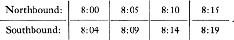
Suppose, further, that the young man usually enters the station at any time during the 5-min intervals. Show that the probability that the “girl in the south” is favored (?) is ![]() . The moral of this problem is not to let chance determine your dates.
. The moral of this problem is not to let chance determine your dates.
17. A term frequently used in discussions of probability is “odds,” which means the ratio of the probability in favor of an event to the probability against the event. What are the odds in favor of throwing a head on a single throw of a coin?
18. What are the odds in favor of throwing at least one head on a single throw of two coins?
The concept of probability which we have examined presupposes that we can recognize equally likely outcomes and then take into account those that are favorable to a certain event. But what is the probability that Jones, now forty years old, will live to be sixty?
One cannot say that the two possible outcomes, life or death at age sixty, are equally likely. One might then try to determine the probability that a person of age forty will die of cancer by the age of sixty, perform similar calculations to determine the probability of death due to other causes, such as heart disease, diabetes, fatal accidents, etc., and, assuming that these probabilities could be determined, somehow manage to combine these partial findings to obtain the final probability that an individual of age forty will live 20 more years. This approach would hardly be successful. Yet the probabilities that, starting from a given age, a man will live any specified number of years are of vital importance to insurance companies. Hence these companies had to find ways of determining life expectancies and mortality rates and they went about it as follows. They collected the birth and death records of 100,000 people, and found, for example, that of 100,000 people alive at age ten, 78,106 people were still alive at age forty. They then took the ratio 78,106/100,000 or 0.78 as the probability that a person of age ten will live to be forty. Of the 78,106 alive at age forty, 57,917 were alive at age sixty. The probability of living from forty to sixty was then taken to be the ratio 57,917/78,106, or about 0.74.
This approach to probability is a basic one. It is, in essence, an appeal to experience to determine the favorable outcomes out of the total number of possible outcomes. Of course, the probabilities so obtained are not exact, but a sample of 100,000 people is large enough to ensure fairly reliable probabilities. The reliance upon experience may seem quite different from the calculation of probabilities based on equally likely outcomes, but the difference is not nearly so great as it may appear to be. Why do we decide that each face on a die is equally likely to show up? Actually it is experience with dice which makes us accept the intuitively appealing argument that all faces are equally likely to appear.
Even though probabilities of life expectancies, accidents of various kinds, and the incidence of diseases are obtained from data based on past experience, once they are obtained, mathematics can be employed to calculate with these probabilities. We saw earlier that the probability of throwing two heads on one throw of two coins or two successive throws of one coin is ![]() ·
· ![]() or
or ![]() . If an insurance company is asked to insure the lives of a husband and wife for a twenty-year period, it is important to know the probability that both will be alive twenty years from the date on which the policy is issued. Let us suppose that both are fifty years old. Now the probability that one person of age fifty will live to be seventy is about 0.55 because of about 70,000 people alive at age fifty, 38,500 are alive at age seventy. The probability that both will live to be seventy can be determined in the same way as the probability of throwing two heads on two throws of one coin, namely, 0.55 · 0.55, or about 0.30. Thus, once the probability that a person of age fifty will live to be seventy has been obtained, mathematics can be employed to calculate the probability that two fifty-year old people will both live to be seventy. The foregoing is a fairly simple, run-of-the-mill problem. As might be expected, mathematics is employed for the solution of far more complicated probability problems arising in insurance. Thus the theory of probability, which was first developed to solve problems of gambling, takes the gamble out of the insurance business.
. If an insurance company is asked to insure the lives of a husband and wife for a twenty-year period, it is important to know the probability that both will be alive twenty years from the date on which the policy is issued. Let us suppose that both are fifty years old. Now the probability that one person of age fifty will live to be seventy is about 0.55 because of about 70,000 people alive at age fifty, 38,500 are alive at age seventy. The probability that both will live to be seventy can be determined in the same way as the probability of throwing two heads on two throws of one coin, namely, 0.55 · 0.55, or about 0.30. Thus, once the probability that a person of age fifty will live to be seventy has been obtained, mathematics can be employed to calculate the probability that two fifty-year old people will both live to be seventy. The foregoing is a fairly simple, run-of-the-mill problem. As might be expected, mathematics is employed for the solution of far more complicated probability problems arising in insurance. Thus the theory of probability, which was first developed to solve problems of gambling, takes the gamble out of the insurance business.
1. How would you determine the probability that a person of age 40 will live to be 60?
2. Of 100,000 ten-year old children, 85,000 reach the age of 30 and 58,000 reach the age of 60. What is the probability that a person of age 10 will live to be 30? What is the probability that a person of age 30 will live to be 60?
3. Suppose that the probability that any one person of age 40 will live to be 70 is 0.5. What is the probability that three particular people of age 40 will live to be 70?
4. Suppose that it is known from long experience that 50% of the people afflicted with a certain disease die of it, say within one year. A doctor who believes that he has developed a new treatment tries it on 4 people and all 4 recover (do not die within one year). How much reliance would you place on the treatment? [Suggestion: What is the probability that 4 people having the disease will recover without any treatment?]
For the problems of probability considered so far, the number of possible outcomes was finite. Thus, for example, the number of possible outcomes in throwing three coins is 8, and the number of people who, out of a total sample of 100,000, may live 20 more years can vary from 0 to 100,000. Let us consider, however, the heights of human beings even if limited to values between 4 ft 6 in. and 8 ft 6 in. The number of possible heights in this range is infinite, since any two heights can differ by arbitrarily small amounts. Moreover we know from experience that all possible values in the range from 4 ft 6 in. to 8 ft 6 in. are not equally likely heights of human beings. What, then, is the probability that a man selected at random is between 70 and 71 in. tall?
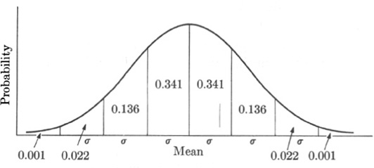
The theory of probability can treat such problems. We shall consider the most important case, namely, where the frequencies of the various possibilities form a normal distribution (Chapter 22). Since we are now thinking in terms of probability rather than, as in the preceding chapter, of a frequency distribution of some quantity such as height or income, we should restate the normal frequency distribution in terms of probability. Let us consider the possible heights of men from the standpoint of the probability of various heights occurring. In our earlier discussion of normal frequency distributions we said that 34.1% of the cases lie within one σ, that is, one standard deviation, to the right of the mean. What this means is that if, for example, the frequency distribution of 1000 heights is normal, then 341 heights would fall within one σ to the right of the mean. If the mean should be 67 in. and σ should be 2 in., then 341 out of the 1000 men would have heights between 67 and 69 in. Then the probability that a man chosen at random out of the thousand has a height between 67 and 69 in. is 341/1000 or 0.341 because the probability is the ratio of the favorable possibilities or outcomes to the total number of possibilities (Fig. 23–1). Likewise, since in a normal frequency distribution 13.6% of all cases (or, one says, of the entire population) lie between σ and 2σ to the right of the mean, it follows that the probability of any individual’s height being between σ and 2σ to the right of the mean is 0.136. In other words, every percentage which appears in the normal frequency distribution becomes a probability under the latter point of view. Thus the normal frequency curve can also be regarded as giving the probabilities of events whose possibilities are normally distributed, and it is therefore also known as the normal probability curve.
Fig. 23–1. The normal probability curve.
We can now answer questions about the probability of events when the frequencies of the various possibilities are normally distributed. For example, given that the heights of men are normally distributed with a mean of 67 in. and a standard deviation of 2 in., what is the probability of finding a man with height greater than 73 in.? Since 73 in. is 3σ to the right of the mean, a height greater than 73 in. is more than 3σ to the right and, as Fig. 23–1 shows, the probability that a height will fall more than 3σ to the right is 0.001; that is, about one man in a thousand is taller than 73 in.
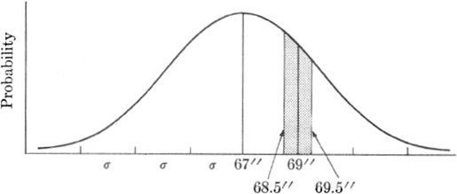
Note that in dealing with infinite populations, we do not ask for the probability of a particular value, for example, the height 69 in. This probability is zero because it is one possibility in an infinite number of possibilities. But the question is not too significant. All measurements yield approximate values only. Let us suppose that the accuracy of measurement is 0.5 in. Then all we should be concerned with is a height between 68.5 in. and 69.5 in.; that is, if we are interested in men with a height of 69 in. and our accuracy of measurement is 0.5 in., then the practical problem we should set is finding the probability that a height falls between 68.5 and 69.5 in. To answer the question, What is the probability that a man chosen at random is between 68.5 and 69.5 in. tall, we would first note that this height lies between 3σ/4 and 5σ/4 to the right of the mean. We would next determine what percentage of the entire population in a normal frequency distribution lies between 3σ/4 and 5σ/4 (Fig. 23–2). We shall not bother to calculate the percentages or the corresponding probabilities which lie within fractional parts of a σ-interval because we wish to restrict our discussion to the simpler percentages or probabilities. However, the probability of a height falling within any given range can be calculated by a method of the calculus.
Fig. 23–2
1. Suppose that the heights of all Americans are normally distributed, that the mean height is 67 in., and that the standard deviation of this distribution is 2 in. What is the probability that any person chosen at random is between 67 and 73 in. tall? between 63 and 71 in. tall?
2. A manufacturer of electric light bulbs finds that the life of these bulbs is normally distributed and that the mean life is 1000 hr with a standard deviation of 50 hr. What is the probability that any bulb chosen at random will fail to burn at least 950 hr?
3. Given the data of the preceding problem, what is the probability that any bulb chosen at random will burn at least 1100 hr?
4. The grades obtained by a large group of students in an examination were normally distributed with a mean of 76 and a standard deviation of 3. What is the probability that a student had a grade between 76 and 79?
5. The weights of a large number of grapefruits were found to be normally distributed with a mean of 1 lb and a standard deviation of 3 oz. What is the probability that any one grapefruit has a weight between 1 lb 3 oz and 1 lb 6 oz?
Let us return for a moment to the subject of tossing coins. When one coin is tossed, there are two possible outcomes: one head and one tail. When two coins are tossed (or one coin is tossed twice), there are four possible outcomes: one yielding two heads, two yielding one head and one tail, and one yielding two tails. When three coins are tossed (or one coin is tossed three times), there are eight possible outcomes: one yielding three heads, three yielding two heads and one tail, three yielding one head and two tails, and one yielding three tails. We could now calculate the total number and distribution of outcomes in tossing four coins, five coins, and so on.
Thinking about this problem of tossing many coins led Pascal to make use of the following “triangle” (now named after him):
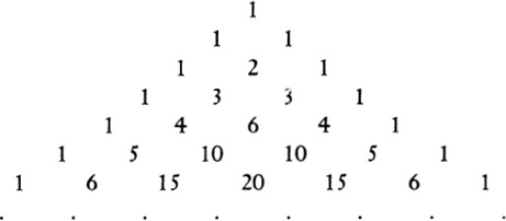
Each number in this triangle is the sum of the two numbers immediately above it (zero must be supplied where one of these two numbers is missing). Thus 4 in the fifth row down is the sum of 1 and 3, and 6 is the sum of 3 and 3. Pascal discovered how well this triangle represents the probabilities of getting heads or tails in throwing coins. Take the case of three coins, for example. The number of possible outcomes is 8, and this is the sum of the numbers in the fourth row. The probabilities involved: ![]() ,
, ![]() ,
, ![]() ,
, ![]() , are obtained from the individual numbers in the fourth row, namely 1, 3, 3, 1. Similarly, the probabilities of the various alternatives which can arise in the process of flipping five coins will be found in the sixth row of the triangle, and so on. (The number 1 in the first row tells us that the probability of winning on a throw of zero coins is 1. This is the only case in which one is certain to win.)
, are obtained from the individual numbers in the fourth row, namely 1, 3, 3, 1. Similarly, the probabilities of the various alternatives which can arise in the process of flipping five coins will be found in the sixth row of the triangle, and so on. (The number 1 in the first row tells us that the probability of winning on a throw of zero coins is 1. This is the only case in which one is certain to win.)
The numbers which appear in the second row, for example, are the coefficients of a and b in a + b, that is, 1 and 1. The numbers which appear in the third row are the coefficients of (a + b)2; for since
(a + b)2 = a2 + 2ab + b2,
we see that the coefficients are 1, 2, 1. The numbers which appear in the fourth row are the coefficients of (a + b)3 for
(a + b)3 = a3 + 3a2b + 3ab2 + b3.
The relationship holds generally. The coefficients of (a + b)n are the numbers in the (n + 1)-row. The quantity a + b is called a binomial because it consists of two terms. Hence distributions which follow any one row of Pascal’s triangle are called binomial distributions.
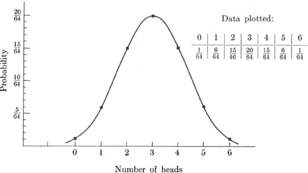
If one wished to calculate the probabilities of the various outcomes in tossing 50 coins, he could employ some standard reasoning in the theory of probability or he could extend Pascal’s triangle to the fifty-first row. It is, however, clear that this latter process is laborious and, as a matter of fact, calculating the various probabilities by means of the formulas of the theory would be equally laborious. There is an alternative. Let us observe the seventh row of Pascal’s triangle. The numbers in this row refer to the throw of six coins, and their sum is 64. Hence they tell us, for example, that the probability of six heads is ![]() ; that of five heads and one tail,
; that of five heads and one tail, ![]() ; that of four heads and two tails,
; that of four heads and two tails, ![]() ; and so on. If we plot the number of possible heads as abscissas and the probabilities of these various numbers of heads as ordinates and draw a smooth curve through the points, we obtain the graph shown in Fig. 23–3. The shape of this graph suggests the normal probability curve. And, indeed, were we to calculate the tenth and the twentieth lines of Pascal’s triangle and plot the corresponding graphs, we would find that as the number of coins increases, the graph of the probabilities of the various outcomes approaches the normal probability curve. For a large number of coins, 20 or more, the approximation is so good that we may as well use all the knowledge we have about the normal probability curve and abandon the calculation of the probabilities by special formulas or by extending Pascal’s triangle.
; and so on. If we plot the number of possible heads as abscissas and the probabilities of these various numbers of heads as ordinates and draw a smooth curve through the points, we obtain the graph shown in Fig. 23–3. The shape of this graph suggests the normal probability curve. And, indeed, were we to calculate the tenth and the twentieth lines of Pascal’s triangle and plot the corresponding graphs, we would find that as the number of coins increases, the graph of the probabilities of the various outcomes approaches the normal probability curve. For a large number of coins, 20 or more, the approximation is so good that we may as well use all the knowledge we have about the normal probability curve and abandon the calculation of the probabilities by special formulas or by extending Pascal’s triangle.
To apply the normal probability curve, we must know the mean and the standard deviation. A glance at Pascal’s triangle shows that the number of heads which has the highest frequency, and therefore the highest probability, is the middle number (or one of the two middle numbers if there is no one middle number). Thus in the seventh row the outcome of 3 heads has the greatest probability. Now this number 3 is the probability of throwing a head, namely, ![]() , multiplied by the number of coins thrown, that is, 6. This example illustrates a general result which we shall state but not prove. If n coins are tossed, the mean number of heads is n/2.*
, multiplied by the number of coins thrown, that is, 6. This example illustrates a general result which we shall state but not prove. If n coins are tossed, the mean number of heads is n/2.*
Fig. 23–3.
Graph of the number of possible heads appearing on a throw of six coins versus probability.
The standard deviation could be determined by applying the procedure for finding the standard deviation of a frequency distribution to the frequencies involved in tossing coins. We would find that
![]()
Both of these results hold for the throw of n coins and do not depend upon our approximating the frequencies of the various numbers of heads by the normal frequency distribution. However, if we do make the approximation, we can use the mean and standard deviation just indicated in connection with the normal frequency curve or with the normal probability curve.
The reader may have the impression that mathematicians have become overly absorbed in coin-tossing and accept this extensive interest as another quirk of queer minds. But, in fact, coin-tossing is merely a useful and concrete example which paves the way for more serious applications. Suppose that the probability of death from a certain disease is ![]() ; that is, half the people who contract the disease die within some definite period of time. A new medical treatment is given to 20 afflicted people and only 3 die within that crucial period. Is the treatment really effective or is it just chance that only 3 out of this group of 20 died? After all, to say that the probability of death from a disease is
; that is, half the people who contract the disease die within some definite period of time. A new medical treatment is given to 20 afflicted people and only 3 die within that crucial period. Is the treatment really effective or is it just chance that only 3 out of this group of 20 died? After all, to say that the probability of death from a disease is ![]() does not mean that in any one group of 20 people 10 will die. It means, as does any probability, that in the long run or in a large number half of those afflicted will die. How should we decide whether the medical treatment is effective?
does not mean that in any one group of 20 people 10 will die. It means, as does any probability, that in the long run or in a large number half of those afflicted will die. How should we decide whether the medical treatment is effective?
The possible outcomes, that is, the possible numbers of those remaining alive without treatment among 20 afflicted people, are precisely the same as the possible outcomes in a throw of 20 coins. Just as the number of heads which may show up can vary from 0 to 20, so among the 20 people, none may live beyond the specified period, one may, and so on up to 20. Since the probability that any one person will remain alive is the same as that of tossing a head on a single throw, the probabilities of the various outcomes will be the same in the two situations. Hence the mean number of those remaining alive is (![]() ) · 20, or 10. The standard deviation of this distribution is
) · 20, or 10. The standard deviation of this distribution is ![]() . In our case,
. In our case,
![]()
Then 3σ to the right of the mean is 10 + 6.72, or 16.72. If we now use the normal probability approximation to our distribution of probabilities (Fig. 23–1), we can say that the probability that more than 16.72 out of 20 afflicted people remain alive without treatment is less than 0.001. But actually 17 people out of the 20 treated remained alive. The probability of this happening in any group of 20 afflicted people is so small that we must credit the treatment with the remarkable record in this group of 20.
Thus when the theory of probability developed for coin-tossing is applied to a serious medical problem, it produces a highly useful conclusion. As a matter of fact, it is precisely this theory which is used to determine the effectiveness of most medical treatments such as the Salk vaccine for poliomyelitis.
Let us consider another application. There is a common belief that boy and girl babies are equally likely or that the probability of a boy being born is ![]() . Suppose that in 2500 births 1310 proved to be boys. Are these data consistent with the accepted probability of one boy in two births? We can answer this question. The possible numbers of boys in 2500 births are precisely the same as the possible numbers of heads in a throw of 2500 coins (or 2500 throws of one coin). Then the mean number of boys is (
. Suppose that in 2500 births 1310 proved to be boys. Are these data consistent with the accepted probability of one boy in two births? We can answer this question. The possible numbers of boys in 2500 births are precisely the same as the possible numbers of heads in a throw of 2500 coins (or 2500 throws of one coin). Then the mean number of boys is (![]() )2500, or 1250. The standard deviation of the distribution of frequencies of these various numbers of boys is
)2500, or 1250. The standard deviation of the distribution of frequencies of these various numbers of boys is ![]() . In our case,
. In our case,
![]()
Now if we use the normal probability distribution as a good approximation to our binomial distribution, we may say that the normal probability curve has a mean of 1250 and a standard deviation of 25. Then 2σ to the right of the mean is 1300. An examination of Fig. 23–1 shows that the probability of 1300 or more boys is 0.023. This means that in only 23 cases out of 1000, on the average, will there be 1300 boys or more in 2500 births.
We are now faced with a problem rather than a conclusion, namely with the occurrence of a very improbable number of births. An event which is very improbable can, of course, occur. However, the entire reasoning is based on the assumption that boy and girl babies are equally likely or that the probability of a boy is ![]() . It seems far more reasonable to question this hypothesis. As a matter of fact, more extensive records show that the ratio of boys to girls is 51 to 49 instead of 50 to 50. This slight difference in ratio makes a lot of difference in the result. Though our theory does not cover this case, we could show that substituting the probability
. It seems far more reasonable to question this hypothesis. As a matter of fact, more extensive records show that the ratio of boys to girls is 51 to 49 instead of 50 to 50. This slight difference in ratio makes a lot of difference in the result. Though our theory does not cover this case, we could show that substituting the probability ![]() for
for ![]() leads to the probability of about
leads to the probability of about ![]() that 1300 or more boys will occur in 2500 births. That an event should occur whose probability is
that 1300 or more boys will occur in 2500 births. That an event should occur whose probability is ![]() is by no means surprising.
is by no means surprising.
In concluding that the medical treatment was effective and in rejecting the hypothesis of equally likely boy and girl births, we relied upon a probability. In the first case we decided that the occurrence of an event whose probability is less than 0.001 implied that the treatment was effective. In the second case we decided that the occurrence of an event whose probability is 0.023 discredited the belief that boy and girl babies are equally likely. The question of what probability to accept as evidence for or against a hypothesis must be decided by the individual concerned, and his judgment will undoubtedly be influenced by the consequences that are likely to arise from his decision.
A recent and most interesting application of the above theory has been made to “prove” the possibility of extrasensory perception, that is, the ability of some people to discern undisclosed facts by extraordinary mental power, for example, to read hidden cards. In the actual tests made by Professor J. B. Rhine and others, subjects were asked to name certain cards held face down, and these people were able to give the correct answers a far greater number of times than the mathematical probabilities of sheer guesses would predict. Thus suppose that the 4 sixes of a deck were held face down on a table. If a subject were asked to select the six of diamonds, he should be able, on the basis of sheer guess, to do so about ![]() of the times. But suppose that the subject selects the right card
of the times. But suppose that the subject selects the right card ![]() of the times in a large number of trials. Such an unexpectedly large ratio of correct choices is interpreted by Rhine to mean an unusual mental faculty, i.e., extrasensory perception. Of course, the argument here centers about the interpretation of the results in the light of the theory of probability. Rhine’s claim is that his experiments also point to telepathy, clairvoyance, prescience, and psychokinesis (the power of the mind to control material objects).
of the times in a large number of trials. Such an unexpectedly large ratio of correct choices is interpreted by Rhine to mean an unusual mental faculty, i.e., extrasensory perception. Of course, the argument here centers about the interpretation of the results in the light of the theory of probability. Rhine’s claim is that his experiments also point to telepathy, clairvoyance, prescience, and psychokinesis (the power of the mind to control material objects).
1. Form the eighth row in Pascal’s triangle and calculate from it the probability of throwing 4 heads and 3 tails in a throw of seven coins.
2. What is the probability of 2 heads in a toss of 6 coins?
3. Suppose that 6 coins are tossed 2000 times. Approximately how often will 2 heads appear?
4. What is the probability of getting at least 5100 heads in a toss of 10,000 coins?
5. Suppose that 50% of people afflicted with a certain disease die. A medical treatment is tried on 100 people, and 65 survive. What is the probability that the treatment is effective?
6. Suppose that the conditions in Exercise 5 are changed to 1000 people of whom 650 survive. Does the probability of the treatment’s effectiveness change? Justify your finding by a qualitative argument.
7. Suppose 860 boys are born in 1600 births. Do these facts support or discredit the hypothesis that boys and girls are equally likely?
8. Suppose 860 heads turn up in a toss of 1600 coins. What conclusion would you draw?
9. The probability that a person of age 40 will live to be 70 is ![]() . Out of 400 people in a certain industry who were forty years old, 150 were alive at the age of 70. What may you conclude about the death rate of workers in this industry?
. Out of 400 people in a certain industry who were forty years old, 150 were alive at the age of 70. What may you conclude about the death rate of workers in this industry?
When one knows the distribution of the probabilities of some variable, one can calculate the probability that a particular value or a range of values will occur and draw a conclusion from this probability. Thus if one knows the distribution of the probabilities of various heights, one can calculate the probability of finding a man with a height, say, between 69 and 70 in. Likewise, if one knows the distribution of the probabilities of the various numbers of heads on a throw of, say 1000 coins, one can calculate the probability of obtaining, for example, 600 or more heads on a particular throw.
In situations of this kind one knows the probabilities of the various alternatives and calculates the probability of a particular one. Now let us consider the following problem. A manufacturer turns out millions of units of the same product each year. He sets up a standard for his product which depends upon the use to which it is put, the price at which it is to sell, the kind of machine which makes it, and other factors. Thus he might decide what, for example, the standard or mean size of his product should be. It is desirable, of course, that all articles produced by one machine be exactly alike, but even under the remarkable accuracy of modern machine performances, complete uniformity cannot be achieved. Hence he also allows for variations, and fixes the standard deviation from the mean which his machinery should hold to. However, machines deteriorate and wear out, or some part may function poorly and affect the output, and the manufacturer therefore checks the output. Since it is too expensive to test each item, he resorts to sampling. Let us say that he examines a sample of 100 units each day. But a sample may have accidental variations which may not be representative of the entire product, just as the mean height of 100 people chosen at random is not necessarily the mean height of all people, even if these people were members of an ethnically homogeneous group. By applying the theory of probability he can decide whether, on the basis of the sample, his machinery is functioning properly, that is, is producing articles with the intended mean and standard deviation.
For the problem of quality control just described, the mean and standard deviation of the entire distribution or population are known, and one judges from a sample whether the mean, say, of the population is being adhered to. There are, however, many problems of sampling in which the mean and standard deviation of the original population are not known, and one is asked to determine them by sampling. For example, a manufacturer of electric light bulbs uses new materials or a new process to make the bulbs and wishes to know how long they will burn on the average. He could test 10,000 bulbs and obtain an answer, but this is not at all necessary. He can test 100 bulbs and find the mean life of this sample. By applying methods of probability theory, which we shall not present, to the mean of his sample, he can determine the mean life of the entire output. The estimate he obtains for the mean of the entire population will not be a precise figure but will lie between certain limits with a probability of almost 1. If he wishes to obtain a better estimate, he can use a larger sample, but the surprising fact is that rather small samples give good estimates of the mean of the entire output.
1. Let us consider a game in which there are 38 possible outcomes (this is true of roulette). Let us suppose that these are numbered 1 to 38. Find the probability
a) that an even number will win,
b) that an odd number will win,
c) that a multiple of four will win.
2. Consider the usual deck of 52 cards. What is the probability in choosing a single card that it will be
a) an ace?
b) a diamond?
c) an ace or a diamond?
3. What is the probability of throwing a 3 or a 5 on a single throw of a die?
4. There are 4 red balls and 3 black balls in an urn. If one ball is drawn, what is the probability that it will be
a) black?
b) red?
c) red or black?
5. An urn contains 4 red balls, 3 black ones, and 2 white ones. Find the probability that a single ball drawn from the urn will be
a) black,
b) red,
c) red or black.
6. a) What is the probability of throwing 2 ones on a single throw of 2 dice? Remember that there are 36 possible outcomes on a throw of 2 dice.
b) What is the probability of throwing an ace twice in two successive throws of a single die?
7. Out of 100,000 people alive at the age of 10 about 70,000 reach the age of 50 and 65,000 reach the age of 55.
a) What is the probability that a 10-year-old child will reach the age of 55?
b) What is the probability that a 50-year-old person will reach the age of 55?
c) Would you conclude from your answers to parts (a) and (b) that the probability of living to the age of 55 is much better at the age of 50 than at the age of 10?
8. Suppose that the heights of American women are normally distributed and that the mean height is 64 in. and that the standard deviation is ![]() in. What is the probability that the height of a woman chosen at random is less than 61 in.?
in. What is the probability that the height of a woman chosen at random is less than 61 in.?
1. Probability applied to games of chance.
2. The evidence for extrasensory perception.
3. The tests of hypotheses by sampling.
4. Probability applied to the study of heredity.
5. The statistical view of nature.
ALDER, HENRY L. and EDWARD B. ROESSLER: Introduction to Probability and Statistics, Chaps. 5 through 9, W. H. Freeman & Co., San Franciso, 1960.
BOHM, DAVID: Causality and Chance in Modern Physics, Routledge & Kegan Paul Ltd., London, 1957.
BORN, MAX: Natural Philosophy of Cause and Chance, Oxford University Press, New York, 1949.
COHEN, MORRIS R. and ERNEST E. NAGEL: Introduction to Logic and Scientific Method, Chaps. 15 and 16, Harcourt Brace and Co., New York, 1934.
FREUND, JOHN E.: Modern Elementary Statistics, 2nd ed., Chaps. 7 through 11, Prentice-Hall, Inc., Englewood Cliffs, 1960.
GAMOW, GEORGE: One Two Three. . . Infinity, Chaps. 8 and 9, The New American Library Mentor Books, New York, 1947.
KASNER, EDWARD and JAMES R. NEWMAN: Mathematics and the Imagination, Chap. 7, Simon and Schuster, Inc., New York, 1940.
KLINE, MORRIS: Mathematics in Western Culture, Chap. 24, Oxford University Press, New York, 1953.
LAPLACE, P. S.: A Philosophical Essay in Probabilities, Dover Publications, Inc., New York, 1951.
LEVINSON, HORACE C.: The Science of Chance, Holt, Rinehart and Winston, Inc., New York, 1950.
MORONEY, M. J.: Facts from Figures, Chaps. 1 through 14, Penguin Books Ltd., Harmondsworth, England, 1951.
ORE, OYSTEIN: Cardano, The Gambling Scholar, pp. 143–241, Princeton University Press, Princeton, 1953.
REICHMANN, W. J.: Use and Abuse of Statistics, Chaps. 14 through 17, Oxford University Press, New York, 1962.
RHINE, J. B.: Parapsychology, Frontier Science of the Mind, Thomas and Co., Springfield, 1957.
SCHRÖDINGER, ERWIN: Science and the Human Temperament, W. W. Norton & Co., New York, 1935. Reprinted under the title Science, Theory and Man, Dover Publications, Inc., New York, 1957.
WEAVER, WARREN: Lady Luck, Doubleday and Co., Inc., Anchor Books, New York, 1963.
* The genes are contained in chromosomes, but here we wish to concentrate, in particular, on the particles which determine color.
* In books on probability, this result is stated in more general form. One may, for example, be dealing with dice, and the probability of throwing ones on each die. This probability is ![]() and the mean number of ones is n/6 or, in general, if p is the probability of the single event, the mean number in n repetitions is np.
and the mean number of ones is n/6 or, in general, if p is the probability of the single event, the mean number in n repetitions is np.