Chapter 2
Theories of the Term Structure of Interest Rates
Tell me, in four words, what is a forward rate?
Interview Question
Chapter 1 introduced the concept of the time value of money. Key to solving the time value of money is the discount rate (i) used to determine either the present or future value of a cash flow occurring at some point in the future (n). Chapter 2 introduces i to the reader. By market convention i may be referred to as the yield curve, the spot rate, or the forward rate. Spot rates, not the yield curve, are used to price bonds and their related derivative contracts. Thus, understanding the derivation of both forward and spot rates is key to understanding the valuation of fixed-income securities.
Typically, the discount rate or i, is derived from a quoted market rate. Given n and i the present or future value of $1 can be determined. The relationship between the discount rate i and the number of periods n is often referred to as the yield curve. The most commonly quoted yield curves are the U.S. Treasury yield curve and the interest rate swap or LIBOR curve.
Generally, as n increases, i also increases but at a diminishing rate. That is, i is an asymptotically increasing function of n. This is often referred to as an upward-sloping yield curve.
The three theories of the term structure of interest rates are:
- The rational or pure expectations hypothesis
- The market segmentation theory
- The liquidity preference theory
Each attempts to explain the following observations with respect to the term structure of interest rates:
- Interest rates across different maturities tend to move together. That is, they are positively correlated.
- The yield curve tends to exhibit a steep positive slope when short-term rates are low and a negative slope when short-term rates are high.
- For the most part, the yield curve exhibits an upward-sloping bias.
Neither the rational expectations nor market segmentation theory fully explain the term structure of interest rates. But, taken together, these theories form the basis of the liquidity preference theory, providing clearer understanding of the term structure of interest rates and the calculation of the discount rates used to value fixed-income securities and their related derivative securities. Thus, the theories of the term structure of interest rates serve as the cornerstone of the relative value analysis that will be presented in following chapters. In the sections that follow, we briefly examine each of these theories.
2.1 The Rational or Pure Expectations Hypothesis
The rational expectations hypothesis asserts that fixed-income investors do not prefer one maturity bond over another [Muth 1961]. That is, investors are indifferent to holding bonds of different maturities. Thus, under the rational expectations hypothesis, bonds of different maturities are considered to be perfect substitutes for one another. This is because under the rational expectations hypothesis, the return on a long-term bond is equal to the expected average of the returns on short-term bonds (forward rates) over the life of the bond.
To illustrate the expectations hypothesis, assume three investment strategies, each with a three-year investment horizon.
- Invest $1 in a one-year bond, and when that bond matures, reinvest the proceeds in a one-year bond in the second and third year as each bond successively matures.
- Invest $1 in a one-year bond, and when that bond matures, reinvest the proceeds in a two-year bond.
- Invest $1 in a three-year bond.
To make this analysis easier, consider a $1 bond that does not offer a coupon but instead pays $1 of principal at maturity. Simplifying the problem to a series of zero coupon securities allows the investor to apply formula 1.1 to each cash flow individually in order to determine the present value of the series of cash flows. This offers the investor the flexibility to assign a unique discount rate, or i—a non-linear term structure assumption—to each cash flow rather than a single i—a linear term structure assumption—as is the case with yield to maturity or the internal rate of return.
The expectations theory states that long-term bond returns are the product of short-term bond returns. Thus, in our example, the expected return of the first strategy can be written as follows:

where:  |
= | the 1-year spot rate |
 |
= | 1-year forward rate, 1 year from today |
 |
= | 1-year forward rate, 2 years from today |
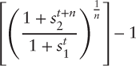
Assume the following spot rate curve given by Table 2.1. The expectations hypothesis states that the two-year spot rate is the product of the one year spot rate and the one year forward rate, one year from today.
Table 2.1 Spot Rate Curve (zero coupon yields)
| Tenor | Spot Rate Curve |
| 1-year | 0.75% |
| 2-year | 1.25% |
| 3-year | 2.00% |
The two-year spot rate is given by:
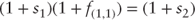
where:  |
= | the 1-year spot rate |
 |
= | the 2-year spot rate |
 |
= | 1-year forward rate, 1 year from today |
Rearranging the terms and solving for the one-year forward rate, one-year from today, results in the following:
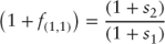
where:  |
= | the 1-year spot rate |
 |
= | the 2-year spot rate |
 |
= | 1-year forward rate, 1 year from today |
The expected one-year forward rate, one year forward, is 0.496% and the expected one-year rate, two-years forward is 0.749% (Table 2.2). If the expected forward rates are realized, then the investor's horizon return will be 2%.

Table 2.2 1-Year Forward Rate in 1 Year
| Tenor | Spot Rate | f(1,1) |
| 1-year | 0.750% | |
| 2-year | 1.250% | 0.496% |
| 3-year | 2.000% | 0.749% |
Alternatively, the investor may decide to purchase a bond with a two-year maturity that yields 2% and invest the proceeds in a one-year bond, two years forward. How would you apply equation 2.4 to show that the investor's expected horizon return is 2%?
In the second strategy presented, the investor purchases $1 of a bond maturing in one year yielding 0.75%, and at its maturity the investor plans to invest the proceeds in a bond maturing in two years. What is the two-year rate, one-year forward?

where:  |
= | the 1-year spot rate |
 |
= | the 3-year spot rate |
 |
= | 2-year forward rate, 1 year from today |
Rearranging the terms and solving for the two-year rate, one year from today (forward), results in the following:
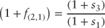
where:  |
= | the 1-year spot rate |
 |
= | the 3-year spot rate |
 |
= | 2-year forward rate, 1-year from today |
The expected two-year rate, one year forward, is 1.249% (Table 2.3). If the expected two-year forward rate is realized, the investor's horizon return will be 2.0%.
Table 2.3 1-Year Forward Rate in 2 Years
| Tenor | Spot Rate | f(1,1) | f(2,1) |
| 1-year | 0.750% | ||
| 2-year | 1.250% | 0.496% | 1.249% |
| 3-year | 2.000% | 0.749% |
The expectations hypothesis explains the first observation with respect to the term structure of interest rates:
- Interest rates tend to move together. For example, if
 increases, then
  also increases, which, in turn, increases the average of the future short-term rates (forwards). Consequently, short-term and long-term interest rates tend to move together.
 - When short-term rates are low and below their average, the market expects short-term rates to go up, and the yield curve exhibits a positive or upward slope. Conversely, when short-term rates are high and above average, then the market expects short-term rates to go down and the yield curve exhibits a negative or downward slope.
2.2 The Market Segmentation Theory
The market segmentation theory asserts that the markets for different maturity bonds are segmented. Under this assumption, the interest rate for each bond is determined by the supply and demand for bonds, without consideration given to the expected returns on bonds of other maturities. Stated differently, under this theory bonds are not substitutable and the expected return from a bond of given maturity has no influence on the demand for a bond of another maturity [Vayanos and Vila 2009].
Further, investors are thought to prefer short-term maturity bonds over long-term maturity bonds. Thus, there is greater relative demand for short-term bonds than there is for long-term bonds. As a result, the price of short-term bonds is higher, resulting in a lower yield than that offered on long-term bonds.
The market segmentation theory explains the tendency of the yield curve to exhibit a positive or upward-sloping bias. However, the market segmentation theory cannot explain the tendency of interest rates to move together, or the presence of downward-sloping yield curves.
2.3 The Liquidity Preference Theory
The liquidity preference theory, like the rational expectations hypothesis, also asserts that bonds are perfect substitutes for one another [Keynes 1936].However, because the investor may be required to sell her bond prior to maturity, thereby assuming interest rate risk, a greater premium is offered to hold longer-term bonds via higher implied forward rates. Simply stated, the liquidity preference theory implies a rational expectation plus a liquidity premium.
In the previous example, the spot rate curve, although upward sloping, implied a lower one-year forward rate. The liquidity preference theory implies higher spot rates than that given by the rational expectations hypothesis. This is because the liquidity premium is assumed to be constant.
Table 2.4 illustrates the derivation of the spot rate curve given a liquidity premium assumption. In the example, the liquidity premium for a “riskless” zero coupon bond with one year to maturity is 0.75%. That is, the one-year spot rate for a risk-free bond is 0.75%. This implies, all else equal, that the one-year spot rate, n periods from today, is also 0.75%. Notice that the spot rate curve implied by the given forward curve in Table 2.4 is steeper than the spot rate curve in the previous example.
Table 2.4 1 Year Forward Rate in 2 Years
| Tenor | Liquidity Premium | f(1,n) | Spot Rate |
| 1-year | 0.75% | 0.75% | |
| 2-year | 0.75% | 1.50% | |
| 3-year | 0.75% | 2.27% |
Since the return on a long-term bond (zero coupon) is equal to the expected average return on short-term bonds (forward rates), one can solve for the spot rate, given a liquidity premium, as follows:

where:  |
= | the 2-year spot rate |
 |
= | 1-year forward rate, 1 year from today |
 |
= | 1-year forward rate, 2 year from today |
The liquidity preference theory incorporates elements of both the rational expectations theory and the market segmentation theory. The liquidity preference theory explains all three observations of the term structure of interest rates:
- Interest rates across different maturities tend to move together. That is, they are positively correlated.
- The yield curve tends to exhibit a steep positive slope when short-term rates are low and a negative slope when short-term rates are high.
- For the most part, the yield curve exhibits an upward-sloping bias.
The use of spot rates to price bonds is complicated by the fact that the market for zero coupon bonds is not liquid. Consequently, it is difficult to observe “market” spot rates. As a result of this, theoretical spot rates are derived from coupon bonds that are quoted along the coupon yield curve. Using the derived spot rates, one is able to price bonds and their related derivatives.
2.4 Modeling the Term Structure of Interest Rates
The remainder of this chapter demonstrates the R package termstrc maintained by Josef Hayden and implemented by Bond Lab®. Readers are encouraged to refer to the article written by Ferstl and Hayden supporting the package. The article provides a definitive description of the methods used to fit the term structure of interest rate [Ferstal and Hayden 2010].
The package termstrc includes all the components required to determine theoretical spot rates. The termstrc package implements the McCullough cubic spline model, the Nelson-Siegel model, as well as extensions to the model. The cubic spline model is non-parametric while the Nelson-Siegel model is parametric.
Parametric term structure models employ an indirect method to derive the required discount rates by fitting the forward curve to derive spot rates. A direct method, like the cubic spline approach, solves for the required discount rates to price bonds. Parametric methods, like Nelson-Siegel, yield output that can be interpreted with respect to the level, slope, and shape of the term structure. As a result, the output from these methods provides some intuition to the investor for understanding the evolution of both the forward and spot rates. It is for this reason that the example presented next implements the Nelson-Siegel model for calculating theoretical forward and spot rates.
The Nelson-Siegel approach for modeling the spot rate curve is outlined by Ferstel and Hayden [Ferstal and Hayden 2010].
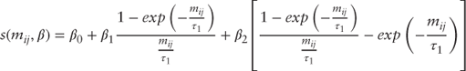
The instantaneous forward rate is given by the following:

where:  , The long-term forward rate , The long-term forward rate |
||
 = The size and location of the hump in the yield curve = The size and location of the hump in the yield curve |
||
 = Location parameter for the hump in the yield curve = Location parameter for the hump in the yield curve |
||
 = Maturity vector = Maturity vector |
Once solved, the parameter vector  allows for the calculation of the spot rate as the average of the forward rates as follows, subject to
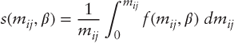
which results in the spot rate function below:
Finally, the discount or present value factor is given by:

The interpretation of the Nelson-Siegel coefficients is as follows:
where:  the long-term interest rate the long-term interest rate |
subject to:  non-negative interest rate constraint non-negative interest rate constraint |
 rate at which the spot rate converges to the long-term slope of the term strutcure rate at which the spot rate converges to the long-term slope of the term strutcure |
 , then a downward-sloping term structure , then a downward-sloping term structure |
 , then a upward-sloping term strucuture , then a upward-sloping term strucuture |
 the size and location of the hump in the yield curve the size and location of the hump in the yield curve |
 then the hump occurs at then the hump occurs at  |
 then the trough occurs at then the trough occurs at  |
2.4.1 Relationship of the Yield Curve to Spot Rates and Forward Rates
The above suggests the following relationship between the yield curve, the spot rate curve, and the forward rate curve.
- When the yield curve is upward sloping, the the spot curve lies above the yield curve and the forward rate curve lies above the spot rate curve.
- When the yield curve is downward sloping, the spot rate curve lies below the yield curve and the forward rate curve lies below the spot rate curve.
2.5 Application of Spot and Forward Rates
Consider the interest rate swap curve quoted as of January 30, 2006, presented in Figure 2.1 [Governors of the Federal Reserve System no date]. Overall, the curve is upward sloping with a inflection point occurring at the two-year maturity. Thereafter, the interest rate swap curve is upward sloping. The 30-year swap rate is 5.08%.
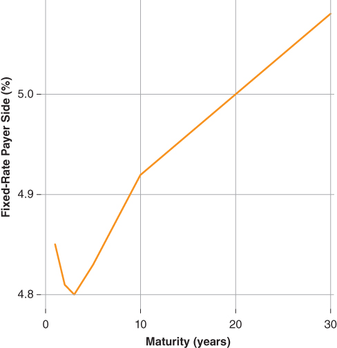
Figure 2.1 Interest Rate Swap Curve, Jan. 30, 2006
Based on our knowledge of the term structure of interest rates, we would expect the following:
- The forward and spot rate curve should slip below the coupon curve at earlier maturities.
- Given the overall upward-sloping bias, both the forward and spot rate curves should cross over and lie above the coupon curve at the later maturities.
Figure 2.2 illustrates both the forward and spot rate curve derived from the Jan. 30, 2006, interest rate swap curve. The spot rate curve follows our intuition as well as the coefficients of the Nelson-Siegel terms.
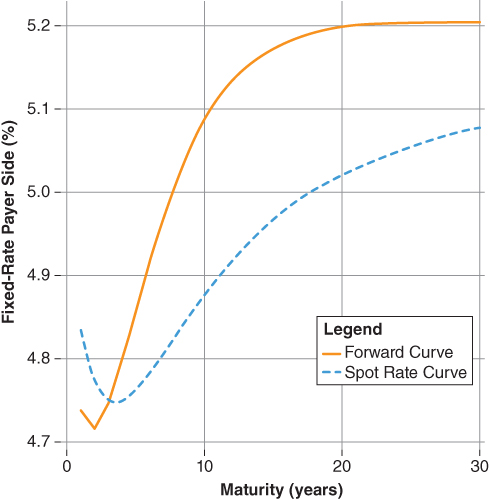
Figure 2.2 Forward and Spot Swap Rates, Jan. 30, 2006
Table 2.5 summarize the model's coefficients. For the most part, the coefficients align with intuition, based on our knowledge of the term structure. The notable exception is  , which suggests that the slope of the term structure is modestly negative. Again, this is due to the inversion of the yield curve between the one-month rate and the two-year rate.
Table 2.5 Nelson-Siegel Terms
| Nelson-Siegel Terms | Value | Interpretation |
 |
5.20 | The long term interest rate is 5.20 |
 |
−0.35 | Implies a downward slope of the term structure |
 |
−0.90 | Implies a trough at  |
 |
3.00 | Implies a trough at 2.6 years |
 |
4.96 | Instantenous short rate |
The coefficients in Table 2.5 follow our intuition with respect to the relationship between the yield (coupon) curve, spot rate curve, and forward rate curve. However, the valuation of fixed-income securities requires that the investor move beyond simply spot rates and one-month forward rates. Given a spot rate curve any forward rate can be derived. It may be necessary for the valuation of certain fixed-income securities to derive a forward rate curve other than the one-month forward rate.
For example, valuing a floating rate bond whose coupon payment is indexed to a rate whose tenor is greater than one-month, like three-month or six-month LIBOR, requires the computation of a similar forward rate. Another example is a mortgage-backed security whose cash flows are contingent on borrower prepayment rates, which are correlated to the prevailing mortgage rate. In the case of a mortgage-backed security, the MBS pool's expected prepayment rate determines the timing of the principal cash flows returned to the investor. The expected prepayment is closely tied to the 10-year swap rate because it influences the prevailing mortgage rate. As a result, the investor is required to calculate the 10-year forward swap rate in order to estimate the forward mortgage rate which in turn motivates her prepayment model (Chapter 9). The above illustrates the extent to which the term structure influences the valuation of structured securities. Indeed, it may be argued, given the extent of the embedded options observed across the structured securities market, a thorough understanding of the term structure is a basic requirement for the valuation thereof.
The forward rate between any two spot rates is given by the equation below:
where:  |
= | The spot rate at  and and  |
 |
= | Beginning time period |
 |
= | Time interval between spot rates |
For example, in Table 2.6 the two-year forward rate in one month (or in the next month) is given by:
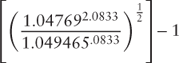
Table 2.6 Calculation of Forward Rates
| Period | Time |
Present Value Factor | Future Value Factor | Spot Rate | 1-Month Forward | 2-Year Forward |
| 1 | 0.0833 | 0.9960 | 1.0040 | 4.9465 | ||
| 2 | 0.1667 | 0.9920 | 1.0081 | 4.9335 | 4.9206 | 4.7616 |
| 3 | 0.2500 | 0.9881 | 1.0121 | 4.9212 | 4.8966 | 4.7521 |
| 4 | 0.3333 | 0.9842 | 1.0161 | 4.9095 | 4.8743 | 4.7436 |
| 5 | 0.4167 | 0.9803 | 1.0201 | 4.8983 | 4.8538 | 4.7361 |
| 6 | 0.5000 | 0.9764 | 1.0241 | 4.8878 | 4.8349 | 4.7295 |
| 7 | 0.5833 | 0.9726 | 1.0282 | 4.8777 | 4.8175 | 4.7238 |
| 8 | 0.6667 | 0.9688 | 1.0322 | 4.8682 | 4.8015 | 4.7189 |
| 9 | 0.7500 | 0.9650 | 1.0362 | 4.8592 | 4.7870 | 4.7148 |
| 10 | 0.8333 | 0.9613 | 1.0403 | 4.8506 | 4.7737 | 4.7114 |
| 11 | 0.9167 | 0.9576 | 1.0443 | 4.8425 | 4.7617 | 4.7087 |
| 12 | 1.0000 | 0.9539 | 1.0483 | 4.8349 | 4.7509 | 4.7067 |
| 13 | 1.0833 | 0.9502 | 1.0524 | 4.8277 | 4.7411 | 4.7052 |
| 14 | 1.1667 | 0.9466 | 1.0565 | 4.8209 | 4.7325 | |
| 15 | 1.2500 | 0.9429 | 1.0605 | 4.8145 | 4.7248 | |
| 16 | 1.3333 | 0.9393 | 1.0646 | 4.8084 | 4.7180 | |
| 17 | 1.4167 | 0.9357 | 1.0687 | 4.8028 | 4.7122 | |
| 18 | 1.5000 | 0.9321 | 1.0728 | 4.7975 | 4.7072 | |
| 19 | 1.5833 | 0.9286 | 1.0769 | 4.7925 | 4.7030 | |
| 20 | 1.6667 | 0.9250 | 1.0811 | 4.7878 | 4.6995 | |
| 21 | 1.7500 | 0.9215 | 1.0852 | 4.7835 | 4.6968 | |
| 22 | 1.8333 | 0.9180 | 1.0894 | 4.7795 | 4.6947 | |
| 23 | 1.9167 | 0.9145 | 1.0935 | 4.7757 | 4.6932 | |
| 24 | 2.0000 | 0.9110 | 1.0977 | 4.7722 | 4.6923 | |
| 25 | 2.0833 | 0.9075 | 1.1019 | 4.7690 | 4.6920 | |
| 26 | 2.1667 | 0.9040 | 1.1061 | 4.7661 | 4.6922 | |
| … | ||||||
| 36 | 3.0000 | 0.8701 | 1.1493 | 4.7484 | 4.7163 |

The two-year forward rate can be confirmed by employing equation 2.1. The horizon return by investing in the one-month spot rate and reinvesting the proceeds at maturity into the two-year forward rate should equal the future value factor of the two-year and one-month spot rate.

The annualized rate of return is:

The spot rate curve is not easily observed in the market. As a result, spot rates are derived from the coupon or yield curve. The spot rate curve implies both present value and future value factors. The present value factors may be used to value periodic cash flows as zero coupon instruments occurring at each point along the spot rate curve. Conversely, the future value factors define both horizon returns for zero coupon bonds as well as the implied forward rates that can be observed between two spot rates. Because of the above properties, the spot rate curve is used to price fixed-income securities and their related credit derivatives.