The great tragedy of science is the slaying of a beautiful theory by an ugly fact.
Thomas Huxley
Countless particles travel in circles under the Swiss countryside, occasionally bumping into each other. All of the effort put into accelerating these particles is in vain if we do not record the collisions between protons by taking what amounts to fast and high- tech photographs. By recording and reviewing millions and indeed billions of these collisions, we will begin to understand what can happen in collisions between protons, from the common to the rare. Finally, by understanding why the common things are common and the rare things are rare, we will learn a great deal about the behavior of matter and energy under extreme conditions and even about the birth of the universe itself.
So just how does one record the collisions caused by a large particle accelerator such as the LHC? You need huge detection equipment, weighing thousands or tens of thousands of tons. In a collision likely to occur in the LHC, two particles enter the collision (the protons) and lots (say somewhere in the neighborhood of 10–500) of particles come out. The story of each collision is etched in the trajectories and the identities of the outgoing particles. Because the actual collision occurs in such a mind- bogglingly short time, the collision itself is usually hidden from us. It’s only by looking at the debris of the collision that we can observe what we need to answer our questions. Understanding particle collisions is essentially a study in forensics.
You can understand the mind- set of an experimental physicist if you pretend to be a bomb- squad investigator. Bomb investigators do not generally understand the details of the explosion by being close by when it occurs—at least not if they want a second assignment. No, bomb investigators understand the explosion by studying its effects on its surroundings. By studying scorch marks, total damage, amount of debris, and how deeply the shrapnel penetrates well-understood materials, the expert can get a good idea as to what happened. Chemical analysis adds to the story.
Similarly, particle physicists study their collisions by surrounding the collision point with a detector of well- known and carefully selected composition. By seeing how the particles leaving the collision interact with the detector, their energy, trajectory, and point of origin can be inferred. The right detector will reveal at least some of the particles’ identities. This information can be brought together like a jigsaw puzzle, with each piece of information neatly interlocking and revealing the true picture of the initial collision.
This chapter begins by discussing the simple building blocks and technical considerations involved in the design of any modern detector. After that, details will be described for each of the major detectors arrayed around the LHC. We will concentrate on the ATLAS and CMS detectors, with fewer details given for the ALICE and LHCb detectors. The TOTEM and LHC- Forward detectors are extensions of ATLAS and CMS and will be mentioned only in passing.
Before we discuss technology and techniques, we must spend a moment talking about the kinds of particles we need to be able to detect. There are literally hundreds of kinds; however, we don’t need to know about all of them to understand the most important points. The handful of particles we need to know about are the electron, the photon, the muon, the neutrino, and a class of particles called hadrons. Electrons and photons are relatively well- known particles, appearing as they do in the familiar world of human experience: electrons in electricity and photons in light. Electrons and photons do not penetrate deeply within a detector.
Muons and neutrinos are less familiar but were introduced in chapter 1. Muons are basically heavy electrons, although they interact very little with the detector and usually pass through it, leaving behind only a small fraction of their energy. Neutrinos have no electric charge, have nearly no mass, and experience only the weak force; they pass through a detector without interacting at all. In essence, they are not seen in a detector and their presence is known only by their absence.
Hadrons are a class of particles that contain quarks within them. The protons and neutrons are the most well- known hadrons, although they are relatively rare in the debris of particle collisions. The most common type of hadrons in a particle collision are called pions, and they can be treated in many ways as if they were light protons, having only about 15% of the mass of a proton. The manner in which hadrons interact with matter is midway between electrons and muons. Hadrons penetrate more deeply than do electrons and photons but not nearly as deeply as muons and neutrinos. The different ways in which these particles interact with matter play an important role in revealing their identity.
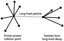
Figure 4.1. Particles that live a long time will travel a considerable distance from the point of common origin or vertex. Thus when you see particles originating from a point other than the one of common origin, you are seeing evidence of a long- lived particle.
Identifying the point of origin of a particle is often very important. This is because sometimes rare particles are made that live for a long time—several trillionths of a second. This seems very short, but highly energetic particles with this lifetime live long enough to travel millimeters or as much as a few centimeters before decaying. Since particles that live this long frequently occur in rare physical processes, you’d like to pinpoint when these kinds of particles are made. Typically, one identifies such events when the trajectory of particles in the event is reconstructed, and it becomes apparent that not all of them originated from the same point that the protons collided. When we project particles back to their point of common origin, we call this a “vertex.” Vertices that differ from the collision point are of interest to physicists. Figure 4.1 shows what the signature of a long- lived particle might look like.
There are many clever techniques for discovering the identity of particles, but we only need to know a few. They have technical names but actually are pretty simple concepts. The topics we will discuss are these: magnetic bending, ionization, showering, and the rather ominous- sounding duo, transition radiation and Cerenkov radiation. We’ll introduce each of these ideas in turn.
The first of the techniques, magnetic bending, is one we’ve encountered already. In chapter 3, we discussed large circular accelerators, which you might recall consisted of a short acceleration region and a vast array of magnets the sole purpose of which is to guide the protons in a circular path back for another acceleration phase. The crucial point here is that charged particles move in a circular path when they are being influenced by a magnetic field.
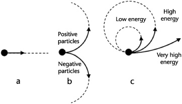
Figure 4.2. The effect of magnetic fields on different kinds of particles. a, A magnetic field does not deflect a neutral particle; b, a magnetic field deflects particles with electric charge, with particles of opposite charge being deflected in opposite directions; and c, particles with low energy travel the circumference of a circle with a small radius and higher energy particles follow circles of larger radii.
This fact can be exploited to help identify and measure the charged particles coming out of a collision. A circle is a simple geometric shape. The only thing that distinguishes different circles is their size. So that having particles traveling in a circular path can be a useful technique for measuring particles, we have to be able to relate a circle’s size (that is radius or circumference) to an important particle property. This turns out to be possible, and the important property is the particle’s momentum. In our ordinary experience, momentum is related to the velocity of the object: the higher the velocity, the higher the momentum.
At the high energies involved in modern particle physics collisions, the correspondence between velocity and momentum doesn’t hold, but it’s still a valuable mental picture. However, in these ultra- violent particle collisions, momentum is more like energy. Because the term is more familiar, I will apologize to my physicist colleagues and use the term energy here.
Because the size of the circular path followed by a charged particle is related to the particle’s energy, by measuring the size of the circle you have simultaneously determined the energy carried by the particle: the bigger the circle, the bigger the energy.
Figure 4.2 illustrates how the energy of a particle is related to the size of the circular path it follows. It also shows another interesting feature. Particles with opposite electric charge (for example an electron and an antimatter electron) curve in opposite directions. If a positive particle moves counterclockwise, a negative particle will move clockwise.
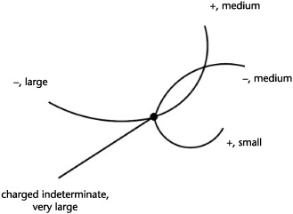
Figure 4.3 shows an example of a relatively simple particle collision. In this example, five particles exit the collision. The particles have different energies and electric charges. From the clockwise and counterclockwise directions of the particles’ motion, we see that we have two particles with positive electrical charge and two negative. The fifth particle has such a large energy that it is difficult to say if it is curving clockwise or counterclockwise. So, because of this ignorance, we are unable to say whether this particle is positive or negative. Further, this particular particle underscores an important limitation of this technique. For instance, if the particle is moving with so much energy that you can’t tell whether it’s moving clockwise or counterclockwise, then that essentially means that it is moving in a nearly straight line.
Figure 4.3. Particles originating from a common origin can be deflected by a magnetic field. In the figure, the (+/–) signs indicate the sign of the electric charge and the words denote the amount of energy they carry. Note the deflection direction and the curvature of the various tracks in relationship to their charge and energy.
Moving in a straight line means that it is moving along the circumference of a huge circle. This means that it has a lot of energy. The problem is that once you get to that much energy, you can’t tell if the circle is huge, super- huge or super- duper- huge. And, if you can’t accurately measure the size of the circle, you can’t accurately determine the particle’s energy.
From this, we see that the magnetic bending technique works best when the energy of the particle isn’t too big. This leads us to wonder how we can accurately measure the energy of highly energetic particles. This question is even more pressing given that we know that the LHC is the highest energy accelerator ever built. Luckily, there is such a technique called showering that works better as the energy of a particle increases. We will explore this technique presently, but first let’s look at the second technique in our list: ionization.
In our discussion of magnetic bending, we learned about the path of a particle and its relationship to the particle’s energy. We didn’t explore exactly how we see the particle. For this, we need to talk about ionization.
When a charged particle passes through a chunk of material, it bounces into the atoms in the material. Now unlike a bowling alley, in which the ball must physically hit a pin to knock it over, the charged particle is surrounded by an electric field. This electric field extends far beyond the size of the charged particle itself. This electric field can reach out and jiggle the atoms of the material through which it is passing.
This is a bit tricky to imagine, so let’s think up some analogies. If you take a magnet and move it near some iron nails, sometimes the nails will be attracted to the magnet, even though the magnet doesn’t actually touch them. Or one might think of a big truck moving down a street covered by newspapers and Styrofoam cups. The wind from the truck’s passage will move the debris around, even though the truck never physically hits it. So too it is with the electric field surrounding a particle carrying an electric charge. As this effectively large object (the charged particle with its extended electric field) plows through material, it bounces into the material’s atoms. With each bounce, the charged particle slows down just a bit, like a bowling ball rolling through a room filled with pins. Fundamentally, that’s all ionization is: a charged particle moves through material, bouncing into the material’s atoms and slowing down in the process.
The next thing you need to know about ionization is that the amount of energy a particle loses is proportional to the distance of matter through which the particle travels. Say the particle loses one unit of energy after traveling through a fixed length of matter (say a centimeter or an inch). Then after traveling through three times that length, it loses three units of energy. Fifteen centimeters (or inches) means 15 units of energy loss and so on. So, conversely, if you measure the distance through which the charged particle travels, you know its energy. In our example above, if a particle travels through 100 cm (or inches) of material and then stops, you know that it had 100 units of energy when it started.
So with those technical concepts out of the way, let’s step back and take a look at what ionization means. For all intents and purposes, it’s the same as slamming on the brakes of your car. The loss of energy as a result of ionization is effectively similar to the loss of the car’s energy as a result of the friction between the tires and the road. And, just like a long skid mark means the car was moving quickly when you hit the brakes (e.g., it had a large initial energy), a charged particle penetrating deeply into matter means its initial energy was large.
So just how deeply can a particle, slowing only by ionization, penetrate into matter? Well obviously that depends on the energy of the particle and the material through which it travels. Taking a relatively low energy particle (10 GeV for the technical types) in solid iron, a particle can travel about 7.6 m (25 feet). Now given that the energy involved in an LHC collision is 14,000 GeV, particles with such a low energy will be very common. Particles with ten times as much energy will be pretty common as well. So these higher (but relatively common) energy particles would require a chunk of iron about a football field deep to stop them.
Given that modern particle physics equipment can’t be that big (imagine a sphere of iron, 180 m, or 600 feet, in diameter around a collision point, costing 10 full years of the entire U.S. federal budget at 2007’s price levels), there must be another solution or different technique we can use. This budget- saving technique is called showering.
While everything we’ve said about ionization is true, for some particles, it’s not the entire story. Some particles will undergo additional types of interactions. The particles in question are electrons, photons, and hadrons (i.e., quark-containing particles). When these particles pass close to an atom, in addition to slowing down through ionization, they can actually split into two or more particles. For instance, if an electron passes close enough to a nucleus, it can kick off a photon: one particle in (electron) and two particles out (electron and photon). Similarly, when a photon comes close to the nucleus of an atom, it can disappear and be replaced by an electron and a positron: again one particle in and two out.
Now here’s a nifty thing. When a particle splits into two particles, they each get (about) half of the energy. So if the distance a particle can penetrate into matter is related to its energy, this splitting has converted one particle that can go a certain distance into two particles that can go half that distance.
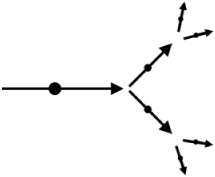
To appreciate showering, you need to know another interesting fact. Once the one particle becomes two particles, well then these two “daughter” particles can also hit atoms and split. In this way, one particle can turn into two, then four, eight, sixteen, and so on. Indeed, it isn’t at all unusual for one particle to “shower” into ten thousand. With that increase in particle count comes a reduction in each particle’s energy. Most important, showering vastly reduces the amount of material needed to fully absorb a particle and measure its energy. The basic idea of showering is shown in Figure 4.4.
The quark- carrying hadrons shower as well, although the details are a bit different. When all effects are taken into account, we find that hadron showers last longer and penetrate more deeply. Roughly speaking, the electromagnetic electron and photon will penetrate several centimeters into a dense material like metal, while hadrons will penetrate a meter or so.
Figure 4.4. Showering. A particle will split into two particles with less energy. Subsequent splits increase the number of particles and reduce the energy of each.
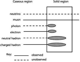
With the introduction of ionization and showering, we can get a first glimpse of how physicists start to distinguish between particle types. Let’s take a simple two- component detector, with one section gaseous and in which ionization is measured and one section solid, in which showering occurs. (Don’t worry about how the ionization is measured, we’ll get to that later.) To show the essential points of how different particles are identified, let’s consider five types: neutrinos, muons, photons, electrons, and hadrons. Neutrinos are electrically neutral and don’t shower. Photons are electrically neutral and shower quickly. Electrons have an electric charge and shower quickly. Hadrons can be neutral or electrically charged and shower slowly. Finally, muons have an electric charge, but don’t shower.
In Figure 4.5, we see that electrically charged particles are observed in the gaseous region, while neutrals are not. In the solid region, particles shower as their nature dictates. By looking at the patterns in both detectors, the identity of the originating particles can be determined with considerable reliability.
Before we get into the specifics of detectors, we need to introduce two additional useful effects: Cerenkov radiation and transition radiation. Most people with even the smallest science interest and training know that you can’t go faster than the speed of light. (Although judging from the crank letters and e- mails I receive every month, this fact is not universally accepted.) Technically, the right thing to say is that you can’t go faster than the speed of light in a vacuum. However, when light travels through a material, it moves more slowly. In fact, light travels through glass or Plexiglas at about two- thirds the speed it has in a vacuum. This fact forms the basis for how lenses, prisms, and any number of optical phenomena work.
Figure 4.5. The different signatures of particles in matter make it possible to distinguish among them. By observing whether the particle ionizes in the gas or showers in the solid, one can fairly reliably identify the particle’s nature. The cross- hatched ellipses indicate a shower. Observed means the detectors will be able to see this particle, while unobserved means that the particle will be invisible to that detector.
That light travels more slowly when moving through glass leaves a loophole in that whole “faster than light” thing. This is because when light hits glass, it slows down immediately (and speeds back up when it leaves the glass). However, the mechanisms that cause the slowing do not affect particles other than the photon. Thus we are left with the following situation: Suppose you had two high energy particles, one electron and one photon, traveling alongside one another in a vacuum. No matter how high the energy carried by the electron, you’d see the photon pull ahead of the electron. If the electron was very high in energy, the photon might inch ahead, but ahead it would pull.
Now send these two particles into a slab of glass. The photon would immediately slow down to about two- thirds its initial speed, while the electron’s speed would be essentially unchanged. Thus in glass, the electron can be faster than the photon! When this happens, an effect occurs that is similar to a sonic boom. A sonic boom occurs when an airplane moves through air faster than sound moves through the same air. Similarly, when an electrically charged particle travels through glass faster than light travels through the same glass, it gives off light. When this light is observed, you can be sure a highly energetic charged particle has passed through the glass. This light is called Cerenkov radiation or Cerenkov light.
We can merge the ideas of Cerenkov light and showering to create a powerful particle detection tool. We will return to this idea later, but suppose you have a block of lead glass, which is used to make any high- end chandelier. Unlike ordinary glass, which is essentially sand that has been melted and cooled, lead glass not surprisingly consists substantially of lead. Recall that when an electron comes close to an atom, it gives off a photon. Further recall that a photon, passing near an atom, will split into electrons and positrons. Finally, recall that these daughter particles can also pass near atoms and that the process will repeat itself. This is the shower we discussed earlier. However, in this case, the shower grows in glass. Because the electrons in the shower are very fast (and exceed the speed of light in glass), the electrons and positrons emit Cerenkov light, which can be collected and converted into electricity for further processing. So a chunk of lead glass and a high- tech electric eye can provide a way to measure the energy of electrons and photons.
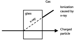
The last technology we’re going to describe is transition radiation. As its name suggests, this is radiation caused by a transition. Ah, but what transition? When a charged particle travels through a medium such as glass, it is surrounded by an electric field that is determined by its own electric charge and by the surrounding medium. However, since the electric field depends in part on the medium through which it travels, the electric field will change as the particle passes from one material to another (say glass to air or plastic to liquid). In the transition from one medium to another, an x- ray photon is emitted from the charged particle. X- rays themselves are not seen, but they have enough energy to interact with the material and induce ionization. Figure 4.6 shows the basic idea.
If you carefully select the materials and the shapes of the materials, you can precisely locate where a charged particle has made the transition. Further, since transition radiation depends on a particle’s velocity, this phenomenon can be used to distinguish fast particles (like the light electron) from slow particles (like the heavy, quark- carrying, hadrons). The ATLAS and ALICE detectors at the LHC use this technology, and we’ll describe how in more detail when we get to the sections in which specific detectors are described.
We now know something about principles important in particle physics detectors: magnetic bending, ionization, showering, Cerenkov radiation, and transition radiation. You may also recall that we want to know as much about the particles coming out from a collision as possible, with special attention paid to their point of origin (usually the place where the collision occurred), their trajectory, electric charge, energy, and identity. It’s now time to bring these ideas together. Obviously there are as many different possible solutions to making the desired measurement with the available technologies as there are clever scientists and engineers. Accordingly, we will restrict the discussion to those choices made as part of the design of the various LHC- based detectors.
Figure 4.6. Transition radiation occurs when a charged particle travels from one kind of material to another. X- radiation is emitted at the transition and these x- rays can ionize a gas for detection.
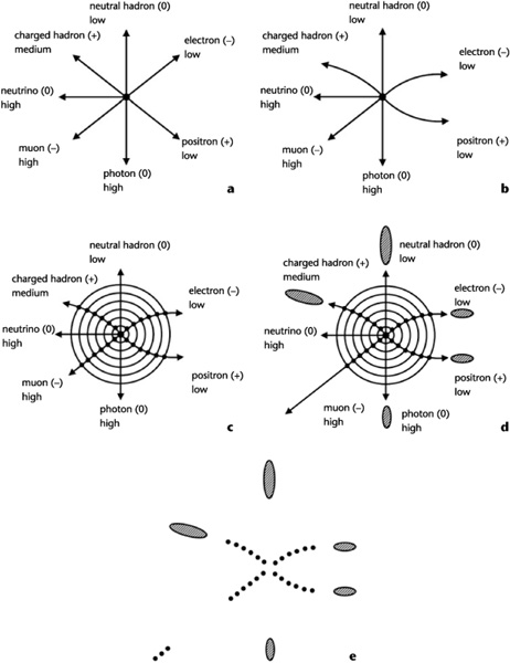
To understand the choices one might make, we first draw a simple cartoon, with only a few kinds of particles. Like the earlier showering discussion, we will include an electron, a photon, a positron (an antimatter electron with the opposite electric charge of an electron), a muon, a neutrino, and both electrically charged and neutral hadrons.
Figure 4.7a shows these particles, when you know everything about them. The identity and electric charge of each particle is given, as is how much energy each one carries. This is what physicists call the truth level. But, of course, our detector doesn’t provide us with this perfect knowledge. In the following paragraphs, we are going to apply some specifics about our newly learned detector knowledge and get an idea of what physicists actually see.
Recall that we want to know the electric charge and energy of the particles. One of the techniques we discussed was magnetic bending. Magnetic bending makes particles with electric charge move in a circular path. The size of the circular path is related to the energy the particle carries. Further, particles with positive electric charge curve in the opposite direction of negative particles.
So let’s apply a magnetic field to the particles of Figure 4.7a and see what effect it has. Figure 4.7b shows how the example particles react to a magnetic field. The low- energy electron and positron are bent a lot. The positively charged hadron with medium energy is bent a middling amount, while the trajectory of the high energy muon is bent only minimally. The other particles, being electrically neutral, are not affected by the magnetic field.
We’ve made our first steps toward understanding a particle scattering collision, but there’s just one obvious problem. We’ve not actually detected the passage of the particles. To do that, we need to dig into our bag of tricks. To view the particles’ paths, we need to use ionization. Recall that ionization occurs when an electrically charged particle crosses through a material and interacts with the material’s atoms. The effect of the particle’s passage is then detected via various methods.
Typically in an ionization detector, you’d like to minimize the total amount of material. If you have too much material, other effects we’ve not discussed (and won’t) come into play and things get complicated rather quickly. So to minimize the amount of material through which the particles must pass, ionization detectors consist of many layers of material, separated by a low density material, such as a gas or vacuum.
In our simple example, we surround the collision with a series of concentric circles of material. Figure 4.7c shows what happens when the detectors are added. Electrically charged particles ionize the material and their passage is recorded, while the neutral particles slip through unscathed. In the figure, the passage of each charged particle through the ionization detector is recorded by a little dot.
So far, we’ve been able to detect electrically charged particles but not the neutral ones. To detect them, we need to add the next trick: showering. Recall that showers provide a way for particles to dump all of their energy rather quickly in a dense material. Electrons, positrons, and photons have short showers, while hadronic particles have longer showers.
Shower detectors are usually comprised of thick slabs of dense material, usually metal. Thick is important, because if the detector is too shallow, the shower might leak out the other side and that means energy would be undetected.
In Figure 4.7d, we see the effect of adding showering detectors. The depth of a shower depends mostly upon the identity of the particle that is causing it. We note that the neutrino has yet to leave a trace in any detector. Further, the muon doesn’t shower and passes through the dense material, leaving only ionization energy. Since the magnetic field isn’t found in the metal, the muon travels in a straight line there. To make sure the particle is a muon, modern detectors typically have a few additional ionization- based detectors outside the showering detector. There may or may not be a magnetic field where the outer ionization detectors are situated. In our simple example, let’s put a magnetic field there.
Figure 4.7e shows this final detector configuration, with knowledge removed of the charge, energy, and identity of the particles that left the signals. Contrast this with Figure 4.7a, where the truth information was revealed. Modern particle experimental physicists train to turn what they can detect (Figure 4.7e) into what was there in the beginning (Figure 4.7a).
So far, we’ve been describing detectors in general terms. Now it is time to get more specific. Our essential questions must be the following: How do we measure the position of a particle? What are the essential components of a showering detector? Let’s start with the first question.
Figure 4.7. a, After a particle collision, particles exit the vertex or point of common origin. Denoted here are the identity, electric charge, and energy of the various particles. b is the same as a but with the effect of a magnetic field imposed. c is the same as b but with a typical ionization detector superimposed. The filled- in dots show where the charged particles traverse the detector and leave a signature. Note that the neutral particles are not observed. d is the same as c but with the showers added. The cross- hatched ellipses show a shower, with the size of the ellipse showing how deep the particles penetrate. Hadron- initiated showers penetrate more deeply than electromagnetically initiated ones. e is the same as d but with all extraneous information removed. Note in three additional ionization detector hits (bottom left), which are from the muon ionization detection system that is outside the shower- measuring device. Compare panel e (which is what is available to the experimenter) with a (which is what we are attempting to observe).
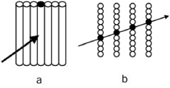
Figure 4.8. A typical ionization detector. Individual detector elements are traversed by a charged particle and signal the particle’s passage. a, face- on view; b, an edge view of multiple planes.
The basis for most position- measuring detectors is ionization. Electrically charged particles cross some material and disturb the electrons in the atoms of the material, and the disturbance is somehow detected. The trick is then to find out where the particle enters the material. While there are a number of choices one can make to accomplish this, by far the most common is to simply make many small ionization detectors, isolate them from one another, and just use your information about which ones were hit to tell you where the particle passed.
As an example, suppose you made a detector somehow composed of ordinary soda straws. Inside each straw is some unspecified material that can be ionized and in which the ionization can be detected. If you took these straws and laid them side by side, they would form the plane seen in Figure 4.8.
Each straw tells us when it is hit. We don’t necessarily know where in the straw the particle passes, but at least we know which one and that tells us something about the particle’s position. If we have many planes of these straws, we can then measure the particle’s path. In Figure 4.8b, we can view many of these planes edge- on and see how the pattern of hit straws gives us the information we need.
Figure 4.8 illustrates an important point. Although the whole “straw” technique can give the necessary position information, a big limitation is the size of the individual straws. Bigger straws measure the position less precisely, while smaller straws give more precise measurements. So it is clear that you should make your straws as small as technologically possible, right? The answer is “Yes, but . . .” This important “but” reminds us of the real- world consideration of cost. Each straw needs its own electronic circuit to read it out, and each circuit adds a cost to the budget. So more straws mean more expense. The reality of fixed budgets imposes a very real limitation on how small one can make the individual straws. In the end, scientists compromise. When precise measurements are critical, they make small detectors and accept the large cost, but when circumstances allow, they use bigger straws and spend their money elsewhere.
In our example, we used a hypothetical detector made of straws. Although there are detectors literally made of straws, that technique is relatively rare. More commonly, scientists use two techniques: wire technology and silicon technology.
In wire technology, the straws are replaced by wires. In fact, a plane of wires looks a lot like a harp. The wires are placed inside a container filled with a carefully chosen gas, and the wire nearest the point where the particle crosses the plane is the one that reports the particle’s passage. The space between adjacent wires varies depending on detector design, but a centimeter or two (a quarter or half an inch) is reasonable. With sophisticated electronics, detectors using this technology can be made to measure a particle’s position with a precision of about a few tenths of a millimeter, or a hundredth of an inch.
To measure more precisely, one must turn to silicon technology. In recent decades, engineers have made enormous strides in minimizing the size of electronic chips for use in computers. This technology can be turned to making particle detectors. In silicon detectors, the “straws” are little strips of silicon, a few centimeters (a couple of inches) long and so narrow that you could fit 20 of them in the space of a millimeter. Recently, it has become economically and technically feasible to make little square “dots” of silicon, 0.05 millimeters on a side. (Although instrumenting these tiny detectors is extraordinarily expensive.)
As I mentioned above, there is a type of detector that uses something that really does look like straws. In this case, charged particles traverse literal straws, filled with material that experiences ionization. As charged particles cross the straws, transition radiation is emitted in the form of x- rays. These x- rays then ionize the material inside the straws and so the particles are detected. The ATLAS detector uses this technology.
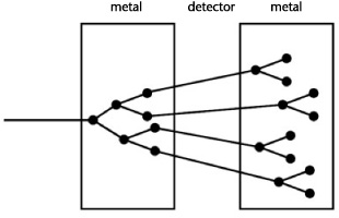
With our discussion of ionization detectors complete, we turn our attention to showering detectors. Showering detectors all have one thing in common. They all consist of dense material. Two techniques are the most common, and the first is called a sampling calorimeter. Its name comes from the fact that it measures a representative sample (sampling) of a particle’s energy (calorimeter). The basic structure of such a detector consists of a series of metal plates, separated by a material in which it is easy to measure ionization energy. This material can be a gas, solid, or liquid, with a density that is lower than that of metal. A typical detector of this form might consist of a plate of steel a few centimeters (an inch) thick, followed by a centimeter or so (half an inch) of the material that actually detects. This pattern might repeat 50 times. The details (thickness and materials used) of any particular detector will vary.
Figure 4.9. In a real sampling calorimeter, the bulk of the showering occurs in high- density metal, while the actual detection occurs in the low- density material between the metal plates.
Figure 4.9 illustrates the important features of a sampling calorimeter. Particles interact with atoms in the high density metal and shower. These shower particles then travel through the active detector material, where the ionization is recorded. The showering begins again in the next metal layer. As this pattern repeats itself, the energy of the individual shower particles drop. Eventually, the energy of the particles drop enough that showering stops. These particles are then simply absorbed and the shower ends. The entire process takes a few billionths of a second.
The second kind of showering detector is called a homogeneous calorimeter. Unlike a sampling calorimeter, a homogeneous calorimeter doesn’t have any structure. The whole detector is the same. To have a detector that can be homogenous, contain metal, and be able to be read out is quite a trick. This is usually accomplished by using some kind of metal- containing glass. The most common form of this kind of glass is lead crystal. That’s right, the same crystal that makes up the chandeliers in a chic hotel’s grand ballroom or in that decanter your mom got for her wedding is an ideal material to be used in a particle detector.
A detector made of lead glass works slightly differently from a sampling calorimeter. A high energy particle enters the glass, traveling faster than the speed of light through the same material. This particle emits Cerenkov light. The particle encounters a lead atom and showers. The daughter particles after the shower are also traveling faster than the speed of light in the glass, so they too emit Cerenkov light. These daughters also encounter lead atoms and the shower grows. The daughter (and granddaughter, and on and on) particles all emit Cerenkov light. Because the detector is made of glass, the Cerenkov light travels to the end of the detector and is collected and converted into electricity. These kinds of metal- containing glass particle detectors are predominantly used to detect electrons, antimatter electrons, and photons.
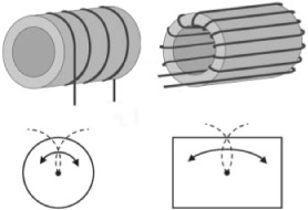
Figure 4.10. Types of magnets: solenoid (top left) and toroid (top right). A solenoidal magnetic field will bend charged particles either clockwise or counterclockwise when the solenoid is seen face- on (bottom left). A toroidal magnetic field will bend the trajectory of charged particles in a plane that includes the side view of the toroid (bottom right). Courtesy Barry Panas.
Because two of the LHC detectors have unfamiliar words in their name, we must make a brief detour into how specific magnetic fields can be made. All magnets in modern particle physics are made by wrapping coils of wire in various shapes. Electric current is passed through the coil, and that current is what generates the magnetic field. These shapes form different kinds of magnetic fields, which in turn bend the particles in different directions. The two most common types of wire- wrapping patterns are the solenoid pattern, in which the wire is wrapped around the outside of a cylinder in the shape of a spring or a “slinky.” A toroid pattern is formed by wrapping the wire in the shape of a bagel. A solenoidal magnetic field bends particles in the plane perpendicular to the beam, while a toroidal magnetic field bends particles toward or away from the beam. Figure 4.10 illustrates these slightly confusing words.
With our discussion of detector techniques complete, we are now able to outline the specific detectors arrayed around the LHC. When the accelerator turns on, there will be two general- purpose detectors designed to study the highest energy proton- proton collisions (CMS and ATLAS). Two additional detectors are designed to study much lower energy phenomena (LHC Forward and Totem). These detectors can be considered to be “add- ons” to the two main detectors. In addition, there will be two other detectors that have been carefully designed to answer much more focused questions. The LHCb detector is optimized to study collisions in which bottom quarks are produced, while ALICE is designed to study the collisions of heavy ions, for instance when lead nuclei are collided together at nearly the speed of light. So let’s introduce each detector in turn.
The rest of this chapter discusses specific detectors stationed at the LHC. Because we are being specific, there are a lot of details given, specifically sizes and number of pieces that go into the individual detectors. If you’re not a detail kind of person, you can skip the rest of this chapter. The principles discussed thus far are featured in various ways in all of the LHC detectors and so you can have a pretty good, although general, idea how all of these detectors work with what you’ve learned to this point. For those of you who are detail- oriented, let’s plunge ahead. We’ll meet up again with the “big picture” people at the start of chapter 5.
The Compact Muon Solenoid, or CMS, detector gets its name because it is relatively small (Compact), is optimized to study muons (Muon), and has a solenoidal magnetic field at its heart (Solenoid). Of course, compact is relative. It’s three stories tall. When we contrast the ATLAS and CMS detectors, the basis of the “compact” term will become more apparent.
Like most modern particle detectors found attached to particle accelerators, CMS (and ATLAS and ALICE) have a layered “onion” structure, with different types of detectors nestled within one another. For simple reasons of engineering, the layers in these detectors are roughly cylindrical in shape, looking like nothing more than a large soup can. The various cylinders representing each type of detector technology are nested together like a series of Russian matrioshka dolls.
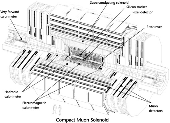
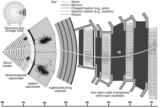
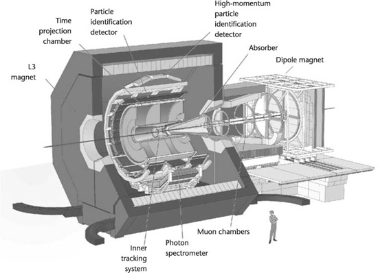
Figure 4.11 shows us the CMS detector. It is 19.8 m (65 feet) long and 14.6 m (48 feet) in diameter and weighs 12,500 tons. It consists of six distinct layers in the “central” or “barrel” region (e.g., the sides of the soup cans) and five distinct layers in the “end cap” regions (e.g., the top and bottom of the can). In the barrel region, these layers consist of the following: two different types of silicon detectors; a calorimeter to measure the energy of electrons, positrons, and photons; a calorimeter for measuring the energy of the quark- containing “hadronic” particles; a magnet; and finally a system for observing muons. The end cap detectors have the same structure except without the magnet. So let’s learn something about these various detectors. The language can be a bit confusing. The equipment that makes up an entire particle physics experiment is called a “detector.” Each experiment consists of many different subsystems, each tasked with a particular purpose. While each subsystem is properly called a “subdetector,” the word “detector” is often used for the overall system, as well as the respective subsystems.
Figure 4.11. A view of the CMS detector, with the various pieces identified. Note the size of the people (drawn to scale) at the bottom. Courtesy CERN and the CMS collaboration.
The silicon tracking detectors of CMS are simply staggering in their technical parameters and are currently without peer. The silicon tracking detectors sit in a volume about 5.8 m (19 feet) long and just under 2 m (a little over 6 feet) in diameter. This volume is not entirely filled with silicon but rather with layers of silicon and air. Each layer of silicon is a fraction of a millimeter thick and is mounted on a cylinder made of a carbon fiber composite. Carbon fiber is used to make modern ultralight airplanes because of its strength. Adjacent cylinders are separated by few centimeters (an inch or two).
The silicon system is broken up into two different subsystems, one consisting of tiny silicon detectors, while the other system consists of super tiny ones. The inner system is called the pixel detector, so- named because it contains super tiny pixels of silicon. To get an idea of what a pixel means, imagine an old- style television. If you were to look closely, you would see that the screen contained little dots, or pixels.
The pixels in the CMS silicon system are much smaller than the TV ones. If one were to look at the pixel detector under a microscope, you’d see that each square millimeter contained about 60 distinct detectors. With such tiny granularity, the CMS pixel detector consists of about 66 million distinct pixels. This incredible number of detectors is spread over a mere three cylinders, about a meter (3 feet) long and ranging in radius from a little under 5 cm (2 inches) to 10 cm (4 inches).
The second CMS silicon detector is much larger. It is 5.8 m (19 feet) long and consists of 10 cylinders ranging in radius from about 20 cm to 1 m (8 to 40 inches). Being so much larger, you’d expect that the number of silicon detectors involved would be much larger, but this apparatus consists of “only” 10 million individual detectors. (I don’t know about you, but to use the words “only” and “million” in the same sentence seems weird to me.) The reason that this system contains so few individual detectors is that each one is much longer. They are called silicon microstrip detectors, so- named because each is a thin strip of silicon about 0.15 mm wide and about 10 cm (a couple of inches) long. Had we lived in a world without resource limitations, we’d have liked to have made just one kind of detector, consisting only of pixels, but cost prohibited that option. So, as we learned in our general discussion of silicon detectors, you make a finely grained detector when you must and make one with larger individual elements when you can.
The CMS silicon detectors cover an enormous area. If you took all of the silicon comprising the CMS detectors and laid it edge to edge, it would entirely cover the floor of an average two- story American house, with just about enough space left over so you could stand and enjoy your handiwork.
For the same reasons that your computer needs a fan, the CMS detector needs to be cold to run well. When silicon is warm, the silicon will generate within itself an unacceptable amount of electric current and stop working. Further, we must use electricity to make the silicon detectors work. Like most simple household appliances, the silicon heats up when powered. When the silicon is working properly it will be operating at about –12°C (10°F).
The next detector one encounters as one moves outward from the center is an unorthodox choice. Ordinarily, the next layer would be the coils through which electric current flows to make the magnetic field. However, in CMS the next layer is the calorimeter used to measure the energy of electrons and photons. Since photons and electrons are electromagnetic particles and the device used to measure energy is called a calorimeter, this device is called the electromagnetic calorimeter, or ECAL.
The ECAL is an example of a homogenous calorimeter. Rather than the lead glass that was discussed in the overview section, the CMS ECAL is made of blocks of lead tungstate (PbWO4 for the chemically minded). Lead tungstate is amazing stuff. While a casual inspection of one of the blocks used in CMS would lead you to believe that it was ordinary, if rather clear, glass, each block is actually 98% metal by weight. Each block is about 2.5 cm (1 inch) in height and width and about 25 cm (9 to 10 inches) long.
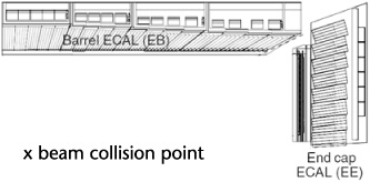
Figure 4.12. A side view of the electromagnetic calorimeter (ECAL). Only a quarter of the detector is shown. The rectangles denote individual lead- tungstate blocks. Courtesy CERN and the CMS collaboration.
Figure 4.12 shows how these blocks are arrayed around the collision point. The ECAL basic shape is a cylinder, with blocks around the barrel and on the end caps. The barrel requires 61,200 blocks and the two end walls 14,648 for a grand total of 75,848 blocks. Taken together, the lead tungstate blocks in CMS weigh about 90 tons.
The next layer in the CMS detector is the hadronic calorimeter, or HCAL. Recall that hadrons are particles containing quarks, of which the proton and neutron are the most familiar. In particle physics collisions, the most common hadrons are pions, which are essentially light protons.
The HCAL is a sampling calorimeter. Like the ECAL, the HCAL is cylindrically shaped with a barrel and ends. The metal most used in the HCAL is brass, although steel is used in a couple of places. Recall that a sampling calorimeter requires layers of metal interspersed with layers of material in which the ionization energy is measured. In the HCAL, this low- density material converts the ionization to light, which is converted in turn to electrical signals. Mostly, the light- producing material is a type of plastic—very similar in appearance to Plexiglas. The layers of metal and plastic consist of plates of brass, 5 to 8 cm (2 or 3 inches) thick, followed by about 0.3 cm (0.125 inches) of plastic.
Recall that the ECAL was made of many blocks of lead tungstate. By knowing which block was hit, you could determine the position where an electron or photon hit the ECAL. The HCAL is conceptually pretty similar, with stacks of metal and plastic effectively making blocks. In CMS, there are 2,592 blocks in the barrel of the HCAL and 2,592 blocks on the ends. In addition, there is another calorimeter very near the beam. This calorimeter is made of steel to make the showers and quartz to make the measurement.
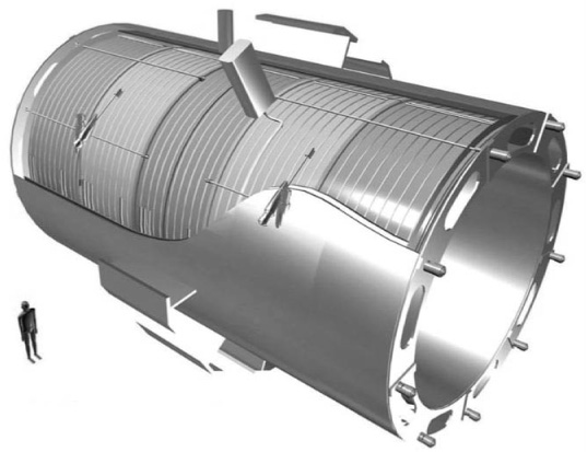
Figure 4.13. The CMS solenoid magnet, the largest one ever made. Courtesy CERN and the CMS collaboration.
Because CMS made the unusual choice to put all the calorimeters inside the magnet, the HCAL isn’t quite as thick as it should be. This is because to make it thicker, the magnet surrounding it would need to be bigger. Since cost considerations made that choice impossible, a few more layers of calorimeter were added onto the outside of the magnet to catch the “tails” of the hadronic showers. The tail of a hadronic shower consists of the few rare particles that penetrate more deeply than usual. This “add- on” calorimeter is aptly called the “tail catcher.”
Between the HCAL and the tail catcher is the CMS magnet, shown in Figure 4.13. The CMS magnet consists of a cylinder with an inner radius of 2.9 m (9.5 feet) and an outer radius of 3.2 m (10.5 feet). The cylinder is about 12 m (40 feet) long and is wrapped 2,168 times with wire. This wire carries the electric current needed to make the magnetic field. The magnetic field in CMS is very strong, about 80,000 times that of the Earth.
To make such a huge magnetic field, about 19,500 amperes of current must pass through this wire. In contrast, most houses need less than 100 amperes. Thus the CMS magnet alone uses over 200 houses’ worth of electricity or about the same as a small suburban neighborhood. To have that much electric current and magnetic field requires an enormous amount of energy (2.7 billion joules for the technically minded), or about enough energy to melt 18 tons of gold. Finally, to keep the wire from vaporizing under the onslaught of that much current, the wire of the magnet needs to be made superconducting. Superconducting, as we recall, means electric current flows without resistance (and thus without heating up the wires). To make the wire superconducting requires it to be cooled to about –269°C (–455°F).
All these technical requirements posed a serious challenge for the CMS engineers. Let’s think a moment about some of the implications of these numbers. With the current required, special accommodations must be made for the power, with a special substation to power the CMS site. In addition, even though the wires of the magnet must be extremely cold, the outside of the magnet must be at room temperature. This means that the magnet must essentially be a large thermos bottle, different only in size from the one that keeps a construction worker’s coffee hot.
Another engineering consequence of the design of the CMS magnet has to do with an inherently self- destructive aspect of designing a large electromagnet. Current makes the magnetic field. However current in a magnetic field feels a force. That’s how electric motors work. So here we have wires that carry current that make a magnetic field. They in turn feel a force and thus want to move. The force is about 2 to 3 tons for every 0.3- m- (foot- ) long segment of the wires that make up the coils. Thus to make the superprecise magnetic field, each segment of wire must withstand the force equivalent to the weight of a mid- sized car. Now recall that the coils of wire comprise 40 km (25 miles) of wire, and you get an idea of the kinds of distorting forces present in the CMS magnet.
Outside the magnet is a series of muon detectors. Because all particles except muons are stopped by the calorimeters, the environment in the muon systems is relatively benign. Unlike the detectors closer to the beam, into which thousands of particles plow every 25 billionths of a second, the muon detectors see only a few.
But for all that, the muon system is still challenging. By far, the muon system is the largest of all of the subdetectors. Its barrel region ranges in radius from about 3.5 to 7 m (12 to 24 feet) and is about 6 m (21 feet) long. The end caps range from 5.5 to 10 m (18 to 34 feet) long and in radius from about 1.4 to 6.7 m (4.5 to 22 feet).
The muon system consists of four thick slabs of iron, interspersed by four layers of position- measuring ionization detectors. Each of these four layers consists of many smaller layers. When all of the individual detectors in the muon systems are counted, they number about 830,000. Figure 4.14 shows a slice of the CMS system, drawn to scale.
Figure 4.14. An edge-on view of the CMS detector with all important detector components and the response of the detector to various types of particles. The path of the muon curves clockwise to the left of the solenoid and counterclockwise to the right after the solenoid because the direction of the magnetic field has changed. The bottom scale indicates the size in meters. The squiggly lines show realistic showers in the electromagnetic and hadronic calorimeters. Each line shows an individual particle in the shower. Courtesy CERN and the CMS collaboration.
The second big detector at the LHC we will discuss is ATLAS (for A Toroidal LHC ApparatuS). The intent of this detector is to study the same kind of collisions as the CMS, with different design choices. Given that nobody knows what kinds of new physical phenomena will be found at the LHC, it seemed prudent to have two competing detectors using different technology.
While the two detectors have appreciable differences, they also have some similarities. This isn’t so surprising, since both detectors are designed to do the same thing: sit at a spot where two beams of protons intersect at their heart and sift through the 20 collisions that occur every 25 billionths of a second and look for something never before seen. So broadly, both detectors are large cylinders, with barrels and ends. At the heart of both detectors are silicon detectors, sitting in a magnetic field. This silicon is surrounded by the energy measuring calorimeters, followed by muon detectors.
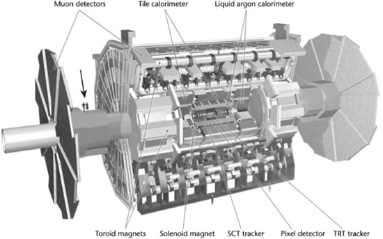
Figure 4.15. The ATLAS detector with components identified. Note two tiny humans on the left on what looks like an axle between the two muon detectors and two more at the base of the detector (drawn to scale). Courtesy CERN and the ATLAS collaboration.
For all their similarities, the two detectors are quite different in detail. The first difference is the physical size. ATLAS is much larger than CMS. CMS is 19.5 m (65 feet) long and 14.5 m (48 feet) wide, ATLAS is 45 m (150 feet) long and 22.5 m (75 feet) wide. So ATLAS’ volume is about six times larger than that of CMS. However, even though the detector is much larger than CMS, it is also much lighter, with a weight of about 7,000 tons (compared with CMS’s 12,500 tons).
ATLAS is shown in Figure 4.15. Its much larger size stems from the designers’ choice to focus on muon measurements. ATLAS’s muon detectors can operate alone, while CMS requires both the muon detectors and the silicon tracker to measure the properties of muons created in its particle collisions. And, as they say, time will tell which choice was best.
The center of the ATLAS detector also consists of silicon pixels. These pixels are about 0.05 × 0.4 millimeters in size. The pixel detector consists of three layers, spread out in a cylinder ranging from about 5 to 25 cm (2 to 10 inches) in radius and a little more than a meter (about 4 feet) long. The ATLAS pixel detector consists of 80 million pixels, somewhat more than CMS’s 66 million.
Outside the volume filled with the pixel detector, ATLAS’s engineers have chosen to put another silicon- based detector. Like CMS, the size of the individual silicon detectors is much larger in this region. These silicon strips are 0.08 mm wide, but about 13 cm (5 inches) long. This detector consists of about 6 million individual silicon detectors and has a cylindrical volume ranging from a radius of 0.3 to 0.6 m (1 to 2 feet) and about 5.5 m (18 feet) long.
Up to this point, the ATLAS and CMS detectors are broadly similar. However, while the CMS detector contains another silicon- based detector with a 1.3- m (40- inch) radius, the ATLAS group chose to use a different technology to fill in this volume.
The next technology encountered as we travel outward from the center of the ATLAS detector is the called the transition radiation detector. The transition radiation detector has a radius of 0.60 to 1m (24 to 41 inches) and is about 5.5 m (18 feet) long. Its basic construction consists essentially of long straws, four millimeters wide and about 0.7 m (28 inches) long. Eight of these straws placed end- to- end cover the entire length of the volume, and filling the entire volume requires 350,000 straws.
These straws are filled by a gas mixture that is mostly xenon. As charged particles cross the straws, they ionize the gas and are detected. However, for very fast particles (usually electrons), x- ray transition radiation is also emitted. This x- radiation also ionizes the xenon gas, leaving an even bigger signal. By seeing which straws are hit, one can follow the trajectory of charged particles through the volume. By seeing which ones have higher or lower signals, one can determine which trajectories are caused by electrons.
While the designers of the CMS detector made the unusual choice to follow the tracker with the lead tungstate ECAL, the ATLAS group made a more traditional choice. The next layer in the ATLAS detector is the central solenoidal magnet, which is similar to that of CMS. The magnet has a radius of a little more than a meter (about 4 feet) and is about 10 cm (4 inches) thick and 5 m (17 feet) long. The wires used to carry the current to energize the electromagnet wrap 1,173 times around the outside of the cylinder and carry a little under 8,000 amperes of current. The net result is a magnetic field of about 40,000 times that of the Earth, or half the magnetic field at the heart of the CMS detector.
Following the ATLAS central magnet are the two calorimeters, the electromagnetic and hadronic. Both calorimeters consist of the usual barrel and end cap geometry. The electromagnetic calorimeter is of the sampling style and uses lead to create the showers and argon, chilled to a liquid form, to measure the shower energy. The ATLAS electromagnetic calorimeter consists of about 175,000 individual detectors, more than double that of CMS.
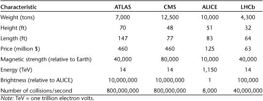
Table 4.1 A comparison of the various major detectors at the LHC
Like in the CMS, the ATLAS calorimeters used to measure hadrons are also sampling calorimeters. In the barrels, layers of iron and ionization- detecting plastic are interleaved, while in the end caps, the structure is copper interleaved with liquid argon. About 19,600 individual detectors make up the ATLAS hadronic calorimeters.
It is when we turn our attention to the final layers of the ATLAS detector, the muon detectors, that we see the greatest contrast with the CMS detector. To begin with, we finally encounter the large toroid magnets that are featured so prominently in ATLAS’s name. The outer ATLAS magnets are enormous. In the central barrel region, the magnets are 24 m (80 feet) long and have a radial distance from 4.6 to 9.8 m (15 to 32 feet). The end cap toroids are 4.8 m (16 feet) long and fill the radial volume from 0.75 to 5.5 m (2.5 to 18 feet). In both sets of magnets, the current is 20,500 amperes. These are big magnets.
The ATLAS muon detection system is similarly impressively large. Various detector technologies record the ionization caused by the muons’ passage. About 1.1 million individual detectors comprise the ATLAS muon system. Figure 4.16 shows a slice of the ATLAS detector.
The two large general purpose detectors at the LHC are amazing, both as feats of engineering and technology. Both detectors are designed to search for new physical phenomena hidden in the deluge of more pedestrian collisions between protons. Table 4.1 summarizes the main points of each detector, each containing nearly a hundred million distinct detector elements. Only time will tell if one group has made better design choices than the other. If history is any guide, both detectors will have an edge over the other in some particular measurements and yet both will make competitive (and superb!) measurements.
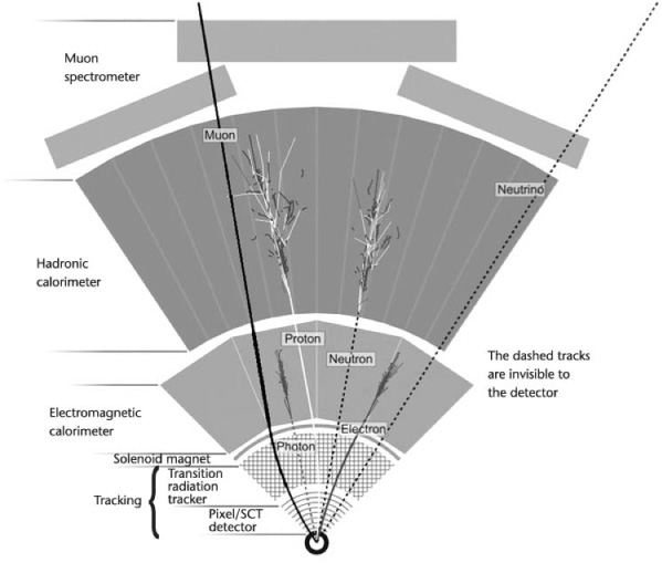
Figure 4.16. An edge-on slice of the ATLAS detector with the important components shown and how they respond to various particle types. Courtesy CERN and the ATLAS collaboration.
One thing we’ve not discussed is the rate at which the two large detectors can collect data. Recall that the proton beams are set up to allow collisions to occur in the center of both detectors every 25 billionth of a second. That means collisions occur 40 million times each second. Further, the beams are so intense that we expect 20 or so collisions every time they pass through one another. That means that there are about 800 million collisions per second in each of the ATLAS and CMS detectors. As my youngest son told me, “Daddy, that’s a lot!”
It turns out that each experiment can record and process about 100 to 200 events per second, a far cry from the 40 million. Roughly speaking, each detector can record only one collision out of every hundred thousand.
Another feature one must consider when attempting to record collisions that are of interest to particle physicists, is that they are extremely rare. Most collisions at the LHC will be relatively gentle impacts between two protons passing by one another, like two strangers brushing shoulders as they pass one another on a street in New York City. However, like the beginning of many a light romantic comedy, in which two hurrying people run head- on into one another, occasionally two protons collide violently, and some interesting physical process is revealed.
The problem is that at the LHC the gentle collisions are about 100 trillion times more likely than the ones we are interested in. Combined with the fact that the LHC experiments can record only one event out of a hundred thousand, this means that one has to be very careful in selecting just what collisions to record. The process whereby one selects events is called a trigger and is crucial to running a successful experiment. If you choose the wrong collisions to record and you don’t have the right data to analyze, you might as well pack it up and go home.
Triggers in a particle physics context are very complex and fluid, so it is impossible to describe them in detail here. The two experiments have made different choices in their initial planning phases, and it is a certainty that by the time you read this, the triggers will be different in detail from what the groups are thinking as I write this. However, there are some essentials that will remain.
The essence of triggering is having a multiple level scheme. Experiments have two to four levels. The basic idea is that data flow into electronics (either custom- built or off the shelf computer components). These electronics are programmed to evaluate the data, decide if they are “interesting,” and pass along for recording the subset of data that seems like it might be worth keeping. Each level makes ever- more- sophisticated decisions.
As an example, we can think what a two- level trigger might be. Level 1 might look to see if detectors in the muon- detection system were hit by the passage of a charged particle. If you’re interested in physical phenomena that produce a muon, well then you can immediately exclude recording collisions in which the muon detectors are silent. The level 1 trigger will make this decision and pass on the events that fit the criteria to level 2.
If it turns out that the muon systems have indicated the passage of a charged particle, this doesn’t necessarily mean that you want to record the event. Recall that the fraction of events that you can record are very small. So the level 2 trigger will look at the subset of events that passed level 1 and stare at them a little harder. Since the number of events entering level 2 is now relatively low, it can spend more time and determine the muon direction, energy, and other characteristics. Then level 2 will decide if the muon passes your criteria and will tell the electronics to discard the event or record it to the computer or other device.
The actual trigger system is much more complicated and looks at different facets of the collisions. But the important points are the same as discussed above. Roughly speaking, the 40 million collisions per second are presented to level 1 for consideration, and about 10,000 events per second are selected as being potentially interesting. Level 2 looks more closely at these 10,000 events and chooses 100 to 200 to record. Later, scientists study these collisions in detail, hoping to see something interesting.
Thus we see that the trigger system is a crucial piece of the design of an experiment. Just like a poor choice in the energy or particle types in your accelerator, or a poor technology choice in your detector can make your experiment a failure, so too can a poor trigger choice. The number of right choices one must make to simply record the data is rather daunting.
The ATLAS and CMS detectors are the large multipurpose detectors that were the primary reason the LHC was built. However, there are other detectors at the LHC, two of which we’ll mention only in passing, and two of which we’ll discuss in a little more detail.
While these first two detectors are attempting to study the rare collisions that may signal new physical phenomena, these particular collisions do not make up the bulk of collisions that occur. Recall that the “interesting and rare” information is about one part per 100 trillion of the collisions. Some scientists are more interested in the common. After all, nobody has measured these common processes at these energies before.
One of the most common things that can happen when protons collide is they act like two billiard balls, just bumping into each other. Two protons enter the collision, and two exit. Because these collisions are relatively gentle, the protons are not scattered at large angles, and so don’t hit the ATLAS and CMS detectors.
Thus two “add- ons” were built that piggyback on ATLAS and CMS. These are small ionization detectors, located near, but outside of, the two big detectors. These detectors record the passage of protons gently bumped out of the beam pipe. The TOTEM detector is associated with CMS, while the equivalent for ATLAS doesn’t yet have a snazzy name. In addition, associated to the ATLAS detector is the LHC forward, or LHCf, detector. This detector is located about 165 m (550 feet) from ATLAS and is designed to look at neutral particles generated very near the beam. These data will help understand common occurrences when protons slam into one another and the cosmic ray collisions discussed in chapter 2. These detectors are very small (a few cubic meters) and are situated a few to hundreds of meters (tens to hundreds of feet) from the big detectors and oriented on the beamline.
Two other major detectors at the LHC remain. While the ATLAS and CMS detectors are designed to be general purpose and versatile, general purpose usually means compromise. Being able to do everything usually means that you don’t do any particular thing as well as you would if you focused on it exclusively.
The ATLAS and CMS detectors are designed to run in the punishing collision environment of having 20 or so proton- proton pairs collide at the same time. These detectors must sift through the debris, looking for some rare physical phenomena. Further, this process repeats itself 40 million times a second. The reason one would design an experiment to run under these conditions is that new physical phenomena are very rare, say one interesting collision for every one hundred trillion boring ones. So in order to have a prayer of seeing anything interesting, you need to simply collide as many proton pairs as possible and hope for good luck. Further, if you want to make sure you understand the new phenomena you see, you need to wrap your detector like a sphere (or a cylinder in the case of ATLAS and CMS) around the entire collision point.
However, for different physics studies, you’d make different choices and nowhere at the LHC is this point made more apparent than in the LHCb experiment. Its main purpose is to study particles containing bottom quarks. These particles are called b- hadrons, where “hadron” means “particles containing quarks” and “b” reminds us that at least one of the quarks is a bottom quark. None of these b- hadrons are something you’ve likely to have heard of before, because they live only briefly—usually about a trillionth of a second.
And yet these short- lived particles can reveal interesting facts about the universe. Studying a class of b- hadrons containing a quark and antiquark, one of them of the bottom quark type, is beginning to shed light on the question of why the universe seems to be composed essentially entirely of matter. Further, it is thought that by precisely measuring the production and decay of b- hadrons that scientists might discover the Holy Grail of something new.
Because events in which b- hadrons are produced are relatively common (occurring in about 1% of all collisions), we don’t have to collide nearly as many protons to study these kinds of collisions. Recall that during normal ATLAS and CMS running about 20 proton- proton collisions occur simultaneously. To accomplish this frantic rate, physicists must make very intense beams and put many protons in each.
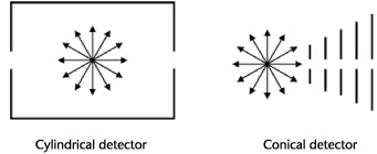
Figure 4.17. A cylindrical detector envelopes the debris of the collision, while a conical detector only samples the debris. These techniques each have their merits, depending on the needs of the measurement. The breaks in the box (left) and the cone (right) show where material is intentionally removed to allow the beam to pass freely.
To study the production of b- hadrons, physicists still use proton beams, but these beams are much less intense than those needed by ATLAS or CMS. In these beams, usually only one pair of protons collides at a time. While the proton collisions still occur 40 million times a second, one collision at a time is much simpler than 20. In addition, the fundamental philosophy of the LHCb experiment is very different from that of ATLAS or CMS. ATLAS and CMS want to record and inspect the entire collision. If some new physical phenomenon is observed, the best way to understand it is to record all of the debris from the collision and inspect it all.
The LHCb experiment is mostly involved in studying b- hadrons. As long as the collision makes a b- hadron or two, that’s a collision scientists might like to study. A corollary of this choice is that the LHCb experiment isn’t concerned with recording all the debris from a collision. As long as the b- hadrons are recorded and measured accurately, that’s good enough. Further, for technical reasons beyond the scope of this book, when b- hadrons are produced, they tend to be “near” the beam. “Near” means they tend to be produced in a narrow cone of about 40°, oriented on the beamline.
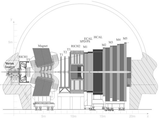
Consequently, the LHCb experiment has a much different geometry than ATLAS or CMS. Rather than a cylinder that envelopes the collision point, LHCb is cone- shaped and oriented to one side of the collision point; b- hadrons fly into the LHCb detector and are analyzed. Many particles created at the LHCb collision point entirely miss the detector. That’s OK, as long as the b- hadrons are recorded. Figure 4.17 contrasts the ATLAS and CMS geometry to that of LHCb. With these introductory remarks in mind, we are now ready to look at LHCb in a little more detail. The LHCb detector is shown in Figure 4.18. You’ll note a resemblance to Figures 4.14 and 4.16. LHCb looks like a slice of its larger counterparts.
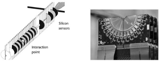
Nearest the collision point is the Vertex Locator, or VELO, detector. The name stems from the detector’s being designed to observe and measure the vertex caused by the b- hadron decay. The VELO detector is made of silicon, with strips about a 0.04–0.10 of a millimeter wide. Altogether, 172,000 strips of silicon make up this detector, compared with the 60 to 80 million detector elements in ATLAS and CMS. The VELO detector consists of 21 distinct layers of silicon, circular in shape and with a hole down the center. The detector has a passing resemblance to a series of CDs stacked and spread out over a meter or so. Figure 4.19 shows the basic mechanics of the VELO detector.
Figure 4.18. An overview of the LHCb detector, with major components identified. Note T1–T3 are the tracking chambers, M1–M5 are the muon detectors, and SPD/PS is a part of the energy-measuring calorimeter system. Figure courtesy CERN and the LHCb collaboration.
The designers of the VELO system made many clever engineering choices, but one is of interest to us here: Unless great care is taken, silicon is susceptible to damage by radiation. In normal operation, the beams would pass through the center of the hole in the center of the VELO disks. However, when the beam is being put into the LHC, it is larger and the danger of mis- steering it is greater. Thus the VELO is split into a left and right side, and the two sides can be retracted during the moments when the beam is unstable and is likely to damage the silicon. In normal running, the VELO detector is positioned a scant 8 mm (0.3 inches) from the beam.
Figure 4.19. A close- up of the LHCb VELO system. Twenty- one disks of silicon surround the interaction point. Figure courtesy of CERN and the LHCb collaboration.
The next detector the debris encounters is one designed to help identify precisely which particles are passing through the LHCb detector. B- hadrons can decay into one particle or another, and precisely measuring how often the various possible decays occur is one of LHCb’s goals. This detector is called a Ring Imaging CHerenkov detector (the designers used the more phonetic spelling of Cerenkov for their acronym), or RICH- 1. The “1” is because there is a second RICH in LHCb (obviously RICH- 2). The rest of the name comes from the fact that Cerenkov light comes out in the shape of a cone surrounding the particle’s passage through the material. Depending on how fast the particle crosses the detector, the cone will be bigger or smaller. This cone of light hits detectors that convert the light to electricity and leaves a circular pattern. So, by measuring the energy of the particle and the size of the circle, one can frequently identify precisely what particle it is. It takes 200,000 photon detector elements in RICH-1 to properly reconstruct the circular patterns.
RICH- 1 is followed by the trigger tracker (TT). This device is made of 180,000 strips of silicon arrayed in four layers. The layers are about 1.2 m (4 feet) high and about 1.5 m (5 feet) wide.
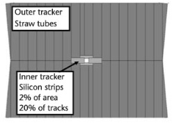
The TT is followed by a strong magnet, the job of which is to bend the path of charged particles traversing it. Once these paths are bent, the charged particles traverse the main tracking system. This system consists of 12 planes, grouped into three stations, each 4.6 m (15 feet) high and 5.8 m (19 feet) wide. This tracking system, depicted in Figure 4.20, consists of the inner and outer trackers. The inner tracker covers only 2% of the total area near the beam. This 2% of the area, while small, is where the particles are most concentrated and captures a full 20% of the particles coming out of the collision. The inner tracker is made of 129,000 silicon strips, about 0.2 millimeters wide and 10 to 20 cm (4 to 8 inches) long. The outer tracker is made of long tubes, filled with a gas that ionizes when charged particles cross them. The outer tracker covers the bulk of the area (98%) with 54,000 tubes.
Figure 4.20. LHCb tracker, highlighting its two- component nature, with a small silicon detector at the heart, followed by a larger tracker consisting of strawlike plastic tubes. While the inner tracker covers only 2% of the detector area, it intercepts 20% of the tracks in a typical particle collision. Courtesy CERN and the LHCb collaboration.
The tracking system is followed by RICH- 2. Its purpose is similar to that of RICH- 1: to help precisely determine the identity of the particles crossing it. RICH- 2 contains 295,000 detector elements.
Just like the other big detectors, the LHCb tracking is followed by the calorimeters and muon- measuring systems. In most detectors, they occur in that order. But in LHCb, the calorimeters and muon system are intermixed, with the first layer of the muon system coming before the calorimeters.
The LHCb calorimeters are pretty traditional and are separated into an electromagnetic and hadronic part, both of the sampling variant. The electromagnetic calorimeter is made of lead to make the showers and plastic to measure the ionization. The hadronic calorimeter consists of layers of iron and plastic. Taken together, the calorimeters consist of a relatively modest 20,000 detector elements.
The final LHCb detector is the five- layered muon system, and it straddles the calorimeter, with one plane coming before the calorimeters and four after. Mostly, the muon system consists of large planes of wires that look like a very large harp. The wires of the harp are surrounded by a special gas that is ionized when crossed by charged particles. The wires carry the ionization energy out to waiting electronics. A small portion of the first layer of muon detectors consists of a technology that allows a more precise determination of the position of the muon’s passage. The muon system’s five planes each consist of about 25,000 different measurements to read out muon positions.
That the LHCb experiment contains something like 1% of the pieces of ATLAS or CMS could be taken to mean that the LHCb experiment is inferior. Nothing can be further from the truth. For about 15% the cost of either of the other two larger detectors, LHCb will capture more than double the number of b- hadrons in any one collision than its larger brethren. This is because the LHCb detector was designed especially to study b- hadrons. When you are not designing for all measurements (and therefore have to be all things to all people), you can focus on your core game and perform better in your own little niche compared with your broader- scoped neighbors.
The last of the big detectors at the LHC that we will discuss in detail is the ALICE (A Large Ion Collider Experiment) detector. Unlike the other three, which are optimized to study the debris of the collisions of proton pairs, ALICE is optimized to study collisions involving lead nuclei. Lead nuclei consist of 208 protons and neutrons, and thus these collisions are much more complex. The energy of the lead beams is immense. While for ordinary proton- proton collisions, the LHC can collide particles with an energy of 14 trillion electron volts of energy, in the case of lead collisions, the total energy is more like 1,150 trillion electron volts.
Given that the total energy involved in lead- lead collisions is 208 times larger than the proton- proton collisions, you might be wondering why people even bother with ATLAS and CMS. The reasons are straightforward. First, the energy in lead collisions is shared between many protons and neutrons. Thus the energy isn’t as concentrated in lead collisions. It’s like comparing the amount of heat in a room as compared to a flaring match. There’s much more heat in the room, but still the match will burn you.
The second reason is that it is difficult to make intense beams of lead. Even working rather hard, the lead beams will only be about 10 million times less intense than the proton beams. Lead beams are so diffuse that even though they will cross as often as proton beams (40 million times a second), the lead beams will only collide about 8,000 times per second. When one insists that the lead nuclei hit head- on and not just a glancing blow, the collision rate will be a paltry 400 times per second, or about 100,000 times less often than the LHCb case and 2,000,000 times less often than in ATLAS and CMS.
With these relatively meager collision rate numbers, it might be a good idea to remind ourselves why we want to collide lead beams. It’s because when a large number of particles are involved, one can observe different behavior. It’s like at the zoo. As long as each species of animal is segregated in its own enclosure, the animals act in a particular way. But magically erase the cages and mix the animals together, then both types of animals, predators and prey alike, will exhibit behavior not seen before they were mixed.
Figure 4.21. Cutaway view of ALICE, with major detector elements highlighted. Note the size of the person in the foreground. Courtesy CERN and the ALICE collaboration.
In a collision between two lead nuclei, 416 protons and neutrons get smashed into a small volume. With the intense heat of such a collision, it is perhaps unsurprising that many thousands of particles come out of the impact; in an extreme case, there can be as many as 20,000. Collisions between lead nuclei are a very messy business.
To study these highly complex interactions, the ALICE group designed and built 15 distinct detectors, using very different technologies. The overarching philosophy of the ALICE detector is not as simple as the cylindrical ATLAS and CMS detectors; nor is it like the conical LHCb detector. Indeed ALICE incorporates most of the tricks used in the other three detectors and a few other creative twists as well. Because the level of detail needed to thoroughly discuss the ALICE detector is so great, I’ve chosen to only sketch the high points of the design.
Figure 4.21 shows the ALICE detector. The detectors near the collision point are a series of cylinders, designed to track particles exiting the collision. Four distinct technologies make up these cylinders. They are a silicon tracker, a detector that utilizes ionization (the time projection chamber, or TPC), a detector that utilizes transition radiation, and a time of flight detector that measures how long it takes for a particle to travel from the collision point to the detector.
Following these detectors are two technologies that don’t cover the entire cylinder. These two detectors are (a) Ring Imaging Cerenkov Counters and (b) lead tungstate crystals. Surrounding these detectors is a huge solenoid magnet. This detector has an abbreviated electromagnetic calorimeter (the lead tungstate crystals) and no hadronic calorimeter at all.
On one end of ALICE, one finds a conical style of detector, designed to measure muons. There are other detectors present in ALICE design, but we’ll neglect to mention them in the interests of brevity. Following this short list of technologies, let’s look briefly the various detectors, starting with the first layer, the inner tracking system or ITS, a silicon- based detector. The ITS sits in a cylinder about 1m (40 inches) long and about 0.9 m (34 inches) in diameter. The system consists of six layers of silicon, with each layer separated by 2.5 to 7.5 cm (1 to 3 inches). Not all layers are the full 1m (40 inches) long, with the layers closer to the beam being shorter. The inner two layers are silicon pixel detectors, while the outer ones are of the strip type. Altogether, the ALICE silicon detector is comprised of about 12.5 million detectors.
The next layer of ALICE uses ionization techniques. Charged particles cross the detector, which is mostly filled with gas. The charged particles ionize the gas by knocking electrons off the atoms. Strong electric fields guide the electrons to waiting electronics. By recording which electronics are hit and by measuring when these ionization electrons arrive, the path of the original charged particles can be determined.
This ionization chamber is the TPC mentioned earlier. It’s a large hollow cylinder, with an inner radius of 0.75 m (2.5 feet) and an outer radius of 2.7 m (9 feet). The cylinder is 4.9 m (16 feet) long, and it contains 560,000 electronic channels.
The next detector utilizes transition radiation and is called the transition radiation detector, or TRD. It fits snugly around the TPC and itself is a hollow cylinder with an inner radius of just over 2.7 m (9 feet) and an outer radius of nearly 3.7 m (12 feet). The cylinder is about 6.7 m (22 feet) long, and the detector consists of about 1.2 million pieces. The purpose of the TRD is to distinguish between fast- moving electrons and the slower (and much, much more common) hadrons seen in collisions between lead nuclei.
The next detector is called a time of flight detector, or TOF. As its name suggests, it measures the amount of time it takes a particle to fly from the collision point to the detector. The basic idea is that one uses the particles’ velocity to determine their identity. If two particles have the same energy, but one particle is much lighter than the other, the lighter particles will move faster and arrive more quickly. Now the differences in arrival times are pretty small. Taking two common hadrons, the difference in arrival time is about 3.5 billionths of a second.
The TOF detector is made mostly of gas and works like most ionization detectors. The difference is the electronics, which include the unusual feature of high- tech stopwatches that record the transit time. The TOF detector is very thin and is a shell about 0.3 m (a foot) thick and 8 m (24 feet) long, wrapped around the TRD. The TOF uses about 160,000 elements.
The next two detectors are odd. They don’t cover the entire cylinder. Instead, they wrap around only a part of the cylinder and are rather short. In both cases, I have the mental image of a blanket on an elephant’s back. The blanket doesn’t fully cover the back, nor does it wrap around his stomach.
The reason these detectors don’t cover the full cylinder are many. First and foremost is that by measuring what one sees in the small area covered by each of these detectors, one can project what’s happening everywhere. Another consideration is cost. A final consideration is that the whole detector needs to fit inside the magnet (the next and final layer of ALICE). There wasn’t enough room to put the two full cylinders in the remaining space.
The first of these two detectors is the high momentum particle identification detector or HMPID. The HMPID is made using Ring Imaging Cerenkov technology, basically similar to the RICH detectors in LHCb. As the name suggests, this detector is intended to determine the identity of highly energetic particles. This detector complements the TOF, which works best at low energy. The HMPID is composed of 161,000 detectors.
The second detector is called the photon spectrometer or PHOS. Like its name suggests, this detector is designed to measure photons. Consisting of 18,000 lead tungstate blocks, each about 2.5 cm (1 inch) square and 18 cm (7 inches) long, this detector has a passing resemblance to the CMS ECAL.
The ALICE detector doesn’t contain a hadron calorimeter or a muon- detection system in its barrel. Instead, the final layer of ALICE is a large solenoid magnet. This magnet has seen service before. Recall that the tunnel in which the LHC accelerator is built used to house the LEP accelerator. The LEP accelerator hosted four experiments: Aleph, Delphi, L3, and Opal. The L3 magnet is now supplying ALICE’s magnetic field.
The L3 magnet has a radius of 4.9 m (16 feet) and is 11.6 m (38 feet) long. The magnet supplies a relatively modest magnetic field, about 10,000 times that of the Earth and about one- eighth that of CMS. However, this lower strength is exactly what is needed for the kinds of particles ALICE will study.
The last major piece of ALICE is a muon detection system. This is not situated around the barrel, but off to one side, broadly similar to the geometry of LHCb. Basically the muon system consists of five boxes, each box containing what look like two harps surrounded by gas. Muons cross the gas and knock electrons from the gas atoms, and the wires guide the electrons to waiting electronics. These five boxes of wires are combined with a magnet. The magnet bends the path of the charged particles and the planes of wires measure the amount of bend. From that, the muon’s energy is measured. The magnet is about one- eighth as strong as CMS, and the muon detection system consists of 1.1 million detectors.
The ALICE detector consists of other subsystems as well, and these detectors play crucial roles in ALICE’s discovery mission. However, these detectors have a more technical interest and a detailed description is omitted here. There are at least nine additional small detectors.
We have now learned something about the four major detectors at the LHC. These four detectors will commence collecting data in 2008 and will be at the forefront of physics research for at least the next two decades. It’s impossible to predict which of the four detectors will make the crucial observation that reveals something entirely new.
Stay tuned!