Prior to the existence of data centers, computing, storage, and the networks that interconnected them existed on the desktop PCs of enterprise users. As data storage grew, along with the need for collaboration, departmental servers were installed and served this purpose. However, they provided services that were dedicated only to local or limited use. As time went on, the departmental servers could not handle the growing load or the widespread collaborative needs of users and were migrated into a more centralized data center. Data centers facilitated an ease of hardware and software management and maintenance and could be more easily shared by all of the enterprise’s users.
Modern data centers were originally created to physically separate traditional computing elements (e.g., PC servers), their associated storage (i.e., storage area networks or SANs) and the networks that interconnected them with client users. The computing power that existed in these types of data centers became focused on specific server functionality, such as running applications that included mail servers, database servers, or other enterprise IT applications.
It was around 10 years ago that an interesting transformation took place. A company called VMware had invented an interesting technology that allowed a host operating system, such as one of the popular Linux distributions, to execute one or more client operating systems (e.g., Windows) as if they were just another piece of software. What VMware did was to create a small program that created a virtual environment that synthesized a real computing environment (e.g., virtual NIC, BIOS, sound adapter, and video). It then marshaled real resources between the virtual machines. This supervisory program was called a hypervisor. This changed everything in the IT world, as it now meant that server software could be deployed in a very fluid manner and also could better utilize available hardware platforms instead of being dedicated to a single piece of hardware. This is shown in Figure 6-1.
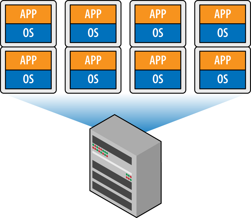
With further advances and increases in memory, computing, and storage, data center servers were increasingly capable of executing a variety of operating systems simultaneously in a virtual environment. Operating systems such as Windows Server that previously occupied an entire bare metal machine were now executed as virtual machines, each running whatever applications client users demanded. Moreover, network administrators now had the option to locate that computing power based not on physical machine availability. They could instead dynamically grow and shrink it as resource demands changed. Thus began the age of elastic computing.
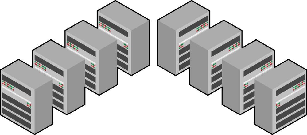
Within the elastic computing environment, operations departments were able to move servers to any physical data center location simply by pausing a virtual machine and copying a file across their network to a new physical computing location (i.e., server). They could even spin up new virtual machines simply by cloning the same file and telling the hypervisor, either locally or on some distant machine, to execute it as a new instance of the same service, thus expanding that resource. If the resource was no longer needed or demand waned, server instances could be shut down or even just deleted. This flexibility allowed network operators to start optimizing the data center resource location and thus utilization based on metrics such as power and cooling. By using bin packing techniques, virtual machines could be tightly mapped onto physical machines, thus optimizing for different characteristics such as locality of network between these servers, or as a means of even shutting down unused physical machines to save on power or cooling. In fact, this is how many modern data centers optimize for virtual machine placement because their dominating cost factors are power and cooling. In these cases, an operator can turn down (or off) cooling an entire portion of a data center. Similarly, an operator could move or dynamically expand computing, storage, or network resources by geographical demand. Figure 6-2 shows a modern data center.
As with all advances in technology, this newly discovered flexibility in operational deployment of computing, storage, and networking resources brought about a new problem: one of operational efficiency both in terms of maximizing the utilization of storage and computing power and in terms of power and cooling. As mentioned earlier, network operators began to realize that computing power demand in general increased over time. To keep up with this demand, IT departments (which typically budget on a yearly basis) would order all the equipment they predicted would be needed for the following year. However, once this equipment arrived and was placed in racks, it would consume power, cooling and space resources—even if it was not used for many months.
The general consensus is that this was first discovered at Amazon. At the time, Amazon’s business was growing at a break-neck rate—doubling every six to nine months. For a while its compute, storage, and network resources could not keep up with the growing demand placed on the company by its online ordering, warehouse, and internal IT systems. For a while, Amazon tried to get ahead of this demand using the old method of prepurchasing a lot of equipment, but ran into the same problems others did in that this equipment would have to be purchased so far in advance that it would in fact sit idle for a significant amount of time. At this point, Amazon realized that while growth had to stay ahead of demand for computing services, it needed to be tailored to be available just in time for their services to use. This is when the idea of Amazon Web Services (AWS) was hatched. Basically the idea was to still preorder capacity in terms of storage, compute, and network, but instead of leaving it idle, the company realized that it could leverage elastic computing principles to sell unused resource pool so that it would be utilized at a rate closer to 100%. When internal resources needed more resources, they would simply push off retail users, and when they were not, retail compute users could use up the unused resources. Some call this elastic computing services—this book calls it hyper virtualization due to the fact that most large data centers do this on quite a massive scale and because the virtualization is so pervasive that this concept is used for storage, computing, and storage resources simultaneously.
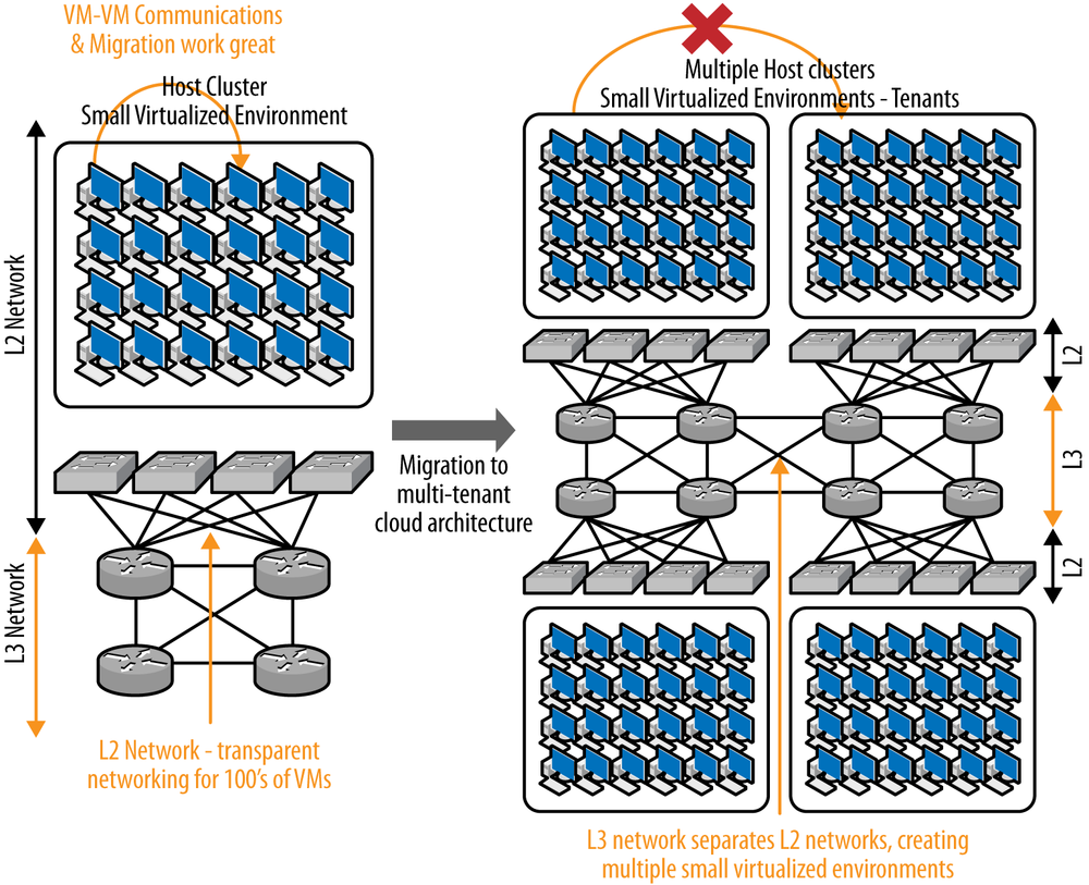
One key thing to notice in the Amazon AWS model is that not only is Amazon virtualizing its services, but in terms of access controls and resources management, it also now needs a different paradigm—by letting external users into its network, it has just created a multitenant data center environment. This of course created a new problem: how to separate potentially thousands of tenants, whose resources need to be spread arbitrarily across different physical data centers’ virtual machines while giving them all ubiquitous and private Internet access to their slice of the AWS cloud? Figure 6-3 illustrates this concept.
Another way to observe this dilemma is to note that during the move to hyper virtualized environments, execution environments were generally run by a single enterprise or organization. That is, they typically owned and operated all of the computing and storage (although some rented co-location space) as if they were a single, flat, local area network (LAN) interconnecting a large number of virtual or physical machines and network attached storage. The exception was in financial institutions, where regulatory requirements mandated separation. However, the number of departments (or tenants) in these cases was relatively small—on the order of fewer than 100. These departments also were addressed using the same, private network IP address space. This was easily solved using existing tools at the time such as MPLS layer 2 or layer 3 VPNs. In both cases though, the network components that linked all of the computing and storage resources up until now were rather simplistic: it was generally a flat Ethernet LAN that connected all of the physical and virtual machines. Most of these environments assigned IP addresses to all of the devices (virtual or physical) in the network from a single network (perhaps with IP subnets), as a single enterprise owned the machines and needed access to them. This also meant that it was also generally not a problem moving virtual machines between different data centers located within that enterprise because, again, they all fell within the same routed domain and could reach each other regardless of physical location.
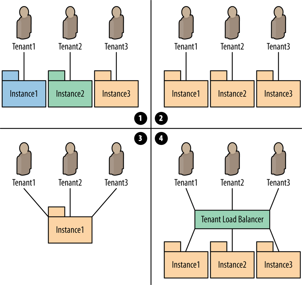
Figure 6-3. Multitenant data center concept; in multitenant data centers, users must have access to virtual slices of compute, storage, and network resources that are kept private from other tenants
The concept of a tenant can mean different things in different circumstances. In a service provider data center providing public cloud services, it means being a customer. In an enterprise data center implementing a private cloud solution, it can mean a department (which can be viewed as an internal customer). Multitenancy is different than multiuser or multienterprise, though not mutually exclusive of these terms. Tenancy occurs above the user or enterprise boundary. Multitenancy is common in both public and private clouds and not limited solely to Infrastructure as a Service (IaaS) data center offerings.
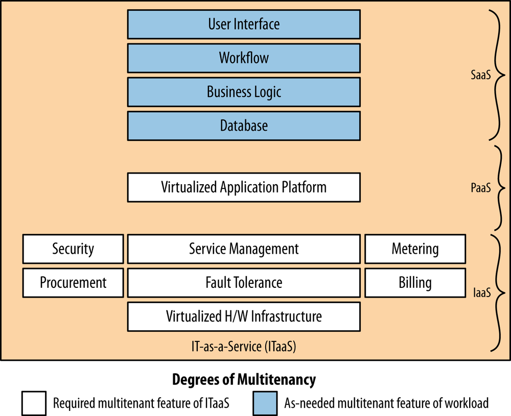
In 2008, when cloud computing was becoming a phenomenon, a blog by Phil Wainewright[127] attempted to define the nuances within the term “multitenancy” as an architectural consideration established at the application layer. A tenant is a user of a shared application environment or (to the point of the blog) some subset of that environment. In the original posting, the differences in the definition of multitenancy were defined as the degree of multitenancy. This concept revolved around how much of the application is shared—down to the database, where the schema defines the database structure. The example given was of Salesforce.com’s deployment of a single schema (shared by all customers) that scaled on a distributed system using database replication technology (at the time of the article, Salesforce was achieving an incredible 1:5000 database instance-to-customer ratio[128]).
By 2012, this idea was revisited, and several notable cloud architects were mapping the degree to common data center application/service archetypes (see Figure 6-4):
- Infrastructure as a service (IaaS)
Infrastructure (compute, storage, and network) are shared. Exemplified by Amazon.
- Platform as a service (PaaS)
An application development environment is shared. Exemplified by Google Apps.
- Software as a service (SaaS)
An application is shared. Exemplified by Salesforce.com.
The architects introduced a second axis of multitenancy (other than the degree to which schema are shared across customers). In this model:
The highest degree of multitenancy occurs in the IaaS and PaaS aspects of the data center service−offering hierarchy.
The overall highest degree of multitenancy occurs when all three aspects of the service offering, including SaaS, are fully multitenant.
A middle-degree of multitenancy may be seen when IaaS and PaaS are multitenant but SaaS is multitenant in physical clusters or for various subcomponents of SaaS.
The lowest degree of multitenancy occurs when SaaS is single tenant.
These degrees describe the tightness of coupling application components and the network and security architectures required to support them—important dependencies related to movement of either a single VM or the distributed-but-dependent collection of application/service components, that is, important to VM mobility—the poster child of SDN applications.
In this chapter, we will explore the basic concepts behind the multitenant data center, associated architecture, and the potential control plane solutions vying to become standards for SDN in the data center.
The virtualized multitenant data center allows multiple tenants to be hosted in a data center while offering them private access to virtual slices of resources. The data center network may be a multitier network. Although the first designs started with a two-layer, spine-and-leaf design, additional growth has caused the appearance of a third, aggregation tier, as shown in Figure 6-5. The data center may also be a single-tier network (e.g., Juniper’s Q-Fabric), as shown in Figure 6-6.
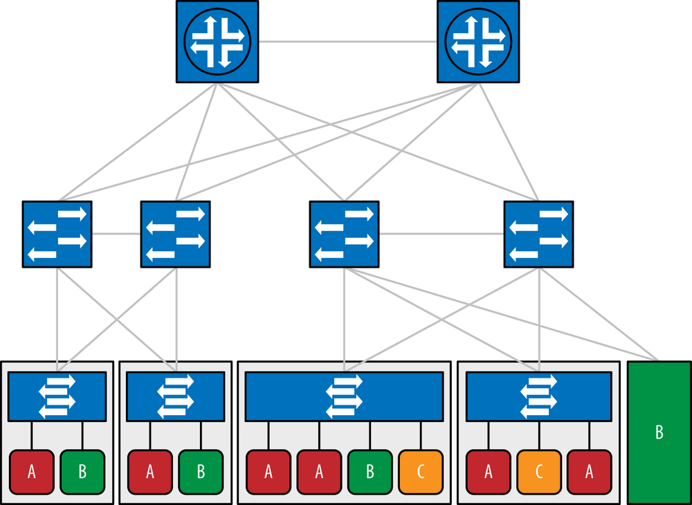
Generally, each tenant corresponds to a set of virtual machines, which are hosted on servers running hypervisors. The hypervisors contain virtual switches (vSwitches) to connect the virtual machines to the physical network and to one another. Applications may also run on a bare-metal server. That is, they are not run in a virtual machine but are instead executed on an entire machine dedicated to that application, as shown in the B server in the lower right corner of Figure 6-6.
Servers are interconnected using a physical network, which is typically a high-speed Ethernet network, although there exist variations where optical rings are used. In Figure 6-5, the network is depicted as a two-tier (access, core) layer 2 network. It could also be a three-tier (access, aggregation, core) layer 2 network, or a one-tier (e.g., Q-Fabric) layer 2 network. For overlay solutions, the data center network could also be a layer 3 network (IP, GRE, or MPLS).
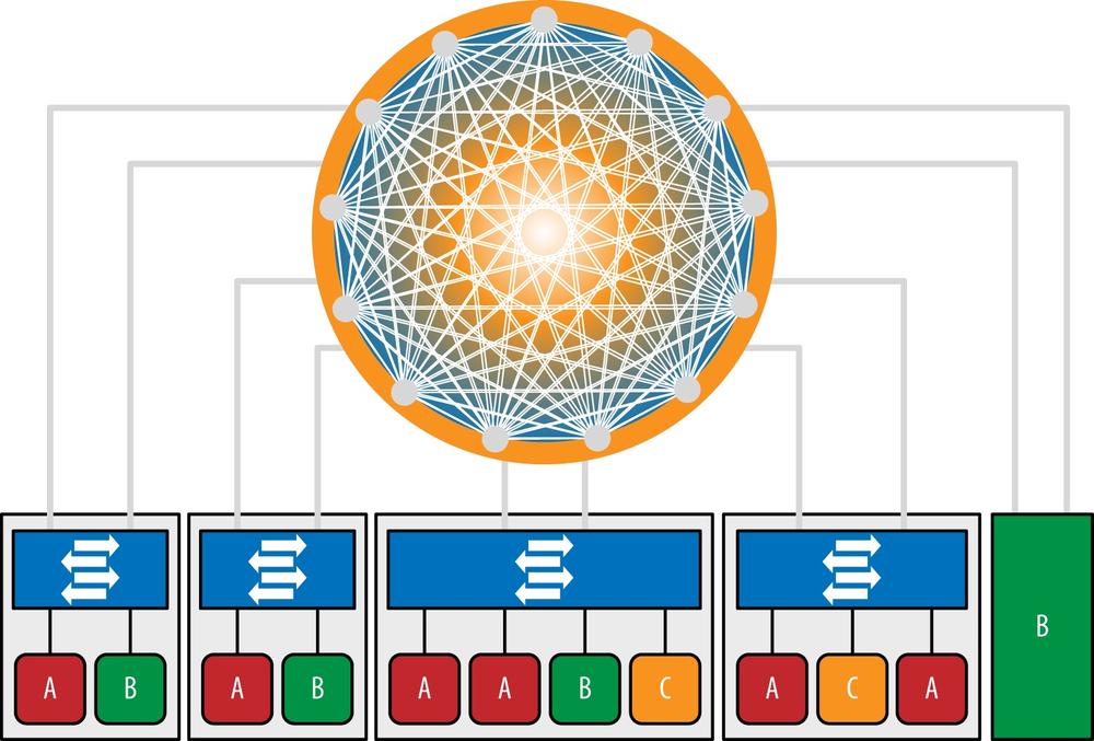
Figure 6-6. Multitenant virtualized data center as a single-tier data center network (Juniper’s Q-Fabric)
Each tenant is assigned a private network, as shown in Figure 6-7. The tenant’s network allows each service instance to communicate with all of the other instances of the same tenant, subject to policy restrictions. In reality, this means that each physical or virtual machine hosting the service must have network access either via layer 3 or layer 2 to the other machines in its logical tenant grouping. The tenant networks are isolated from one another: a virtual machine of one tenant is not able to communicate with a virtual machine of another tenant unless specifically allowed by policy.
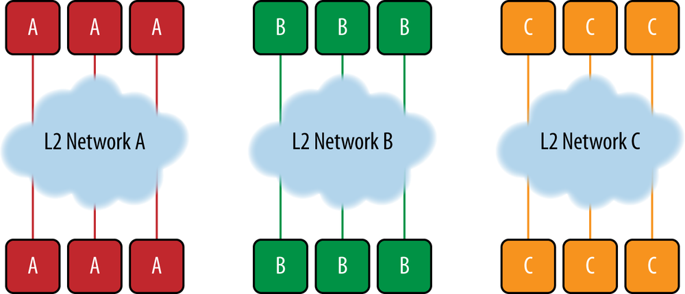
The tenant private networks are generally layer 2 networks, and all virtual machines on a given tenant network are then configured within the same layer 3 IP subnet. The tenant may be allowed to pick his own IP address for the VMs, or the cloud provider may assign the IP addresses. Either way, the IP addresses may not be unique across tenants (i.e., the same IP address may be used by two VMs of two different tenants). In these cases, some network address scheme (NAT) must be employed if those tenants are allowed to speak to each other or others outside of that network (such as public Internet access to the services).
A single tenant may have multiple networks, for example, for the purpose of implementing security zones, for combining multiple departments together such as in a case where IaaS is in use, or when multiple cloud providers are being utilized to host their services. Figure 6-8 illustrates how multiple cloud providers are attached to an enterprise’s local data center in order to extend their data center, thereby providing elastic cloud services. The advantages of this configuration include redundancy, use of the cheapest cloud providers resources (much like consuming electricity from multiple providers is done), or simply to provide geographic coverage for services deployed over a wide geographic span.
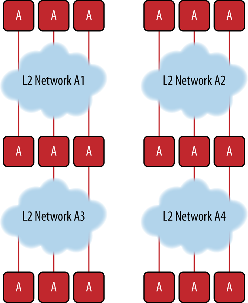
Figure 6-8. Multiple networks for a tenant enterprise; tenant cloud networks A1, A2, A3, and A4 span multiple geographic and logical service providers to weave together a consistent yet virtual service offering for customer A
One important aspect of a virtualized multitenant data center solution is orchestration. In order for a service provider to deploy and otherwise manage a multitenant data center solution, it must implement some form of logically centralized orchestration. Orchestration in a data center provides the logically centralized control and interaction point for network operators and is a central point of control of other network controllers. At a high level, the orchestration layer provides the capability of:
Adding and removing tenants
Billing system interface after provisioning operations are executed
Workflow automation
Adding and removing virtual machines to and from tenants
Specifying the bandwidth, quality of service, and security attributes of a tenant network
This orchestration layer must cover all aspects of the data center that include interfacing with compute, storage, network, and storage systems or controllers. And it must do so at a high rate of change to support true elastic compute services, as demonstrated in Figure 6-9.

Data center tenants are typically connected to the Internet or the tenant’s enterprise network via some VPN, as shown in Figure 6-10. The VPN can be a L3 MPLS VPN, a L2 MPLS VPN, an SSL VPN, an IPsec VPN, or some other type of VPN. The actual type of VPN has different pros and cons and also depends on which underlay network is employed in the data center (such as Ethernet, VLANs, stacked VLANs, VxLAN, and MPLS). The various types of underlays and network overlays will be discussed in detail later in this chapter.
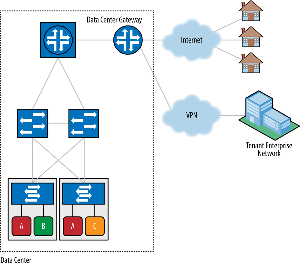
The data center gateway function is responsible for connecting the tenant networks to the Internet, other VPN sites, or both, as shown in Figure 6-10. Note that multiple gateways may be employed, depending on the network architecture employed. While it is still typical to deploy physical devices as gateways, it is also perfectly viable to implement the gateway function in software as a virtualized service. We discuss this more in Chapter 7.
Virtual machine (VM) migration is the act of moving a VM from one compute server to another server. This includes cases where it is running but can also include dormant, paused, or shutdown states of a VM. In most cases, the operation involves what ultimately is a file copy between servers or storage arrays close to the new computing resource (but proximity does not have to be the case).
The motivations for VM migration include:
Data center maintenance
Workload balance/rebalance/capacity expansion (including power management)
Data center migration, consolidation or expansion
Disaster avoidance/recovery
Geographic locality (i.e., moving access to a service closer to users to improve their experience)
Given the earlier definition of tenancy and the concept of the degree of tenancy, the idea that migration is limited to a single server instance is the simplest case to illustrate. In some cases, the application may be multitier and represented by a tightly coupled ensemble of VMs and network elements. Migration of a single VM in this context could lead to performance and bandwidth problems. The operator and/or orchestration system needs to be aware of the dependencies of the ensemble. However, in other cases, where there is a loose coupling of the various layers of an application (i.e., compute, frontend load-balancer/web-services, and a backend distributed database), much as applications written to take advantage of Hadoop or other granular process distribution architectures, VM migration—or more commonly, destruction and creation, usually only has beneficial effects on the service. In these cases, live VM migration is typically not employed. The three-tiered architecture is shown in Figure 6-11. In the three-tiered architecture, a single VM is required to implement each of the three layers of the system, but more component VMs can be spun-up at any time to execute either locally on the same compute server or remotely in order to expand or contract computing resources. Seamless job process distribution is handled by technologies such as Hadoop, which enables this granular and elastic computing paradigm while seamless, easily scalable, and highly resilient backend database functionality is handled by technologies such as Cassandra.
There is still some debate about how frequently live migration might occur between data centers as a DCI use case. The reasoning is that in order for any migration to take place, a file copy of the active VM to a new compute server must be performed, and while a VM is being copied, it cannot be running, or the file would change out from under the copy operation. Hence this operation is becoming less and less common in practice. Instead, moving to a three-tiered application architecture where the norm is to create and destroy machines is far simpler (and safer).
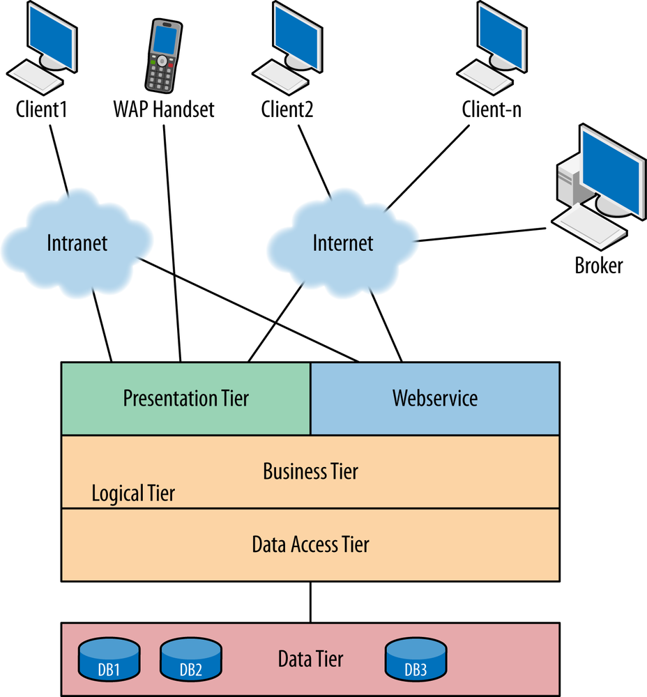
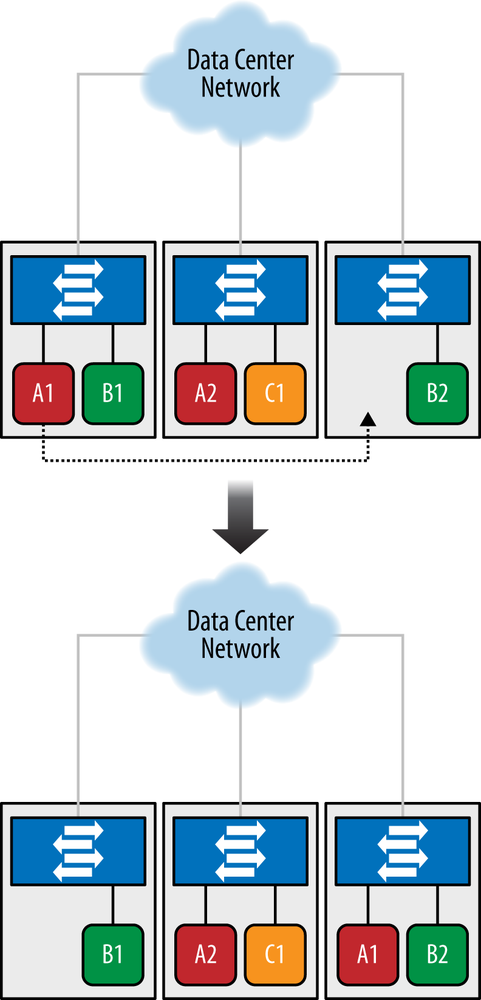
Figure 6-12 demonstrates a VM move between two compute servers. If the two servers are in the same data center, it is an intra data center VM migration requiring a simple point-to-point file copy of the VM file after pausing the VM. If the two servers are in different data centers, it is referred to as an inter data center VM migration and still requires a file copy between two IP end points but may require that file transfer to traverse a much more complex and lengthy network path. Based on this, and remembering the discussion regarding live VM moves, in order for the VM to remain live during the file transfer, the network must continue running throughout the migration, and all sessions (e.g., TCP connection) must remain up. This is a bit of wizardry handled by the hypervisor system that manages the VMs and the VM move.
Further complicating the situation is that in many cases, the MAC address and the IP address of the VM must remain unchanged, as well as any configuration state related to the VM, in order to facilitate a seamless move. This includes other network-related items such as QoS configuration, ACLs, firewall rules, and security policies. All of these things must be migrated to the new server and/or access switch. This also includes any runtime state inside the VM itself and in the vSwitch. In addition, the switches in the physical network must be promptly updated to reflect the new position of the VM. This includes MAC tables, ARP tables, and multicast group membership tables. It is for these complications that it is far easier to employ the three-tiered application design pattern and simply create and destroy component VMs.
The VM migration can be implemented in one of three ways:
- Network Data-plane driven approach
VM migration can be detected through the supporting network devices monitoring network traffic to and from the VM (for example, detection of gratuitous ARP messages).
- Hypervisor driven approach
The component inside the hypervisor (the vSwitch or the vGW) uses introspection to detect the VM migration. One way to do this is by virtue of the old hypervisor detecting that the VM is gone while the new hypervisor detects the VM has appeared.
- Orchestrator driven approach
The VM migration is not detected at runtime a priori; instead, the orchestrator explicitly triggers the movement of runtime state before it performs the VM migration.
The runtime state can be updated in one of two ways:
- Data-plane driven approach
The VM sends some traffic to force the runtime state to be updated. For example, the VM can broadcast a gratuitous ARP to force all MAC tables in the tenant network to be updated with the new location of the VM’s MAC address.
- Orchestrator or control-plane driven approach
The orchestrator uses a control-plane signaling protocol to explicitly update the runtime state in all places where it needs to be updated.
Note
The details of the specific method for detecting a VM migration and updating the runtime state are provided in the section SDN Solutions for the Data Center Network.
VM migration is implemented by copying the entire state (disk, memory, registers, etc.) from one server to another. This is generally accomplished by copying the VM’s file that includes all of these things in a single file. During the initial phase, which can take several minutes, the copying process occurs in the background while the VM is still running on the original server. In the last fraction of a second, when the copying is almost complete, the original VM is suspended, the last remaining state is copied, and the VM is reanimated on the new server. This process requires high bandwidth and low latency between the two servers because the time it takes to replicate this last state equates to time that the service implemented by the VM is unresponsive.
An alternative approach is to take a snapshot of a VM, pause it, and then move the snapshot to another server, after which the hypervisor will un-pause the VM. This is a migration, but not a live migration.[129] There is an aspect related to storage in live migration, particularly if the two VMs use the shared storage model in which both VMs share a common logical volume on a common physical disk (array) and transfer a lock that allows I/O to continue during migration. Distance and latency allowed for this procedure varies with the disk access protocol (iSCSI, NFS, Fibre Channel). It is also possible to again split the application into multiple tiers whereby a common backend database is used to store state and other information. Just before the VM pauses before its move, that state is locked. When it reanimates elsewhere, it simply reconnects to this store and continues.
Scale and performance of VM moves will vary based on the type of service offering (IaaS, PaaS, or SaaS) and the degree of tenancy. A simple IaaS offering at a typical service provider with the current generation of Intel/ARM processor, c. 2012, might present the following rough scale numbers:
- Number of data centers
Multiples of tens (depends entirely on the geography of the offering; the example given would be for a country the size of Japan)
- Number of servers per center
Tens of thousands
- Number of servers per cluster/pod
1,000
- Number of tenants per server
Approximately 20 (current generation of processor, expected to double with next generation)
- Number of VMs per tenant
Approximately five
- VM change rate
Highly variable
- VM change latency
This is a target that varies by provider and application
Now that we have introduced the basic concepts of what a data center is and how one can be built, let’s discuss how one or more data centers can be connected. In particular, for configurations where multiple data centers are required either for geographic diversity, disaster recovery, service, or cloud bursting, data centers are interconnected over some form of Wide Area Network (WAN). This is the case even if data centers are geographically down the street from one another; even in these cases, some metro access network is typically used to interconnect them. A variety of technological options exist that can achieve these interconnections. These include EVPN, VPLS, MPLS L3 or L2 VPNs, pseudowires, and even just plain old IP.
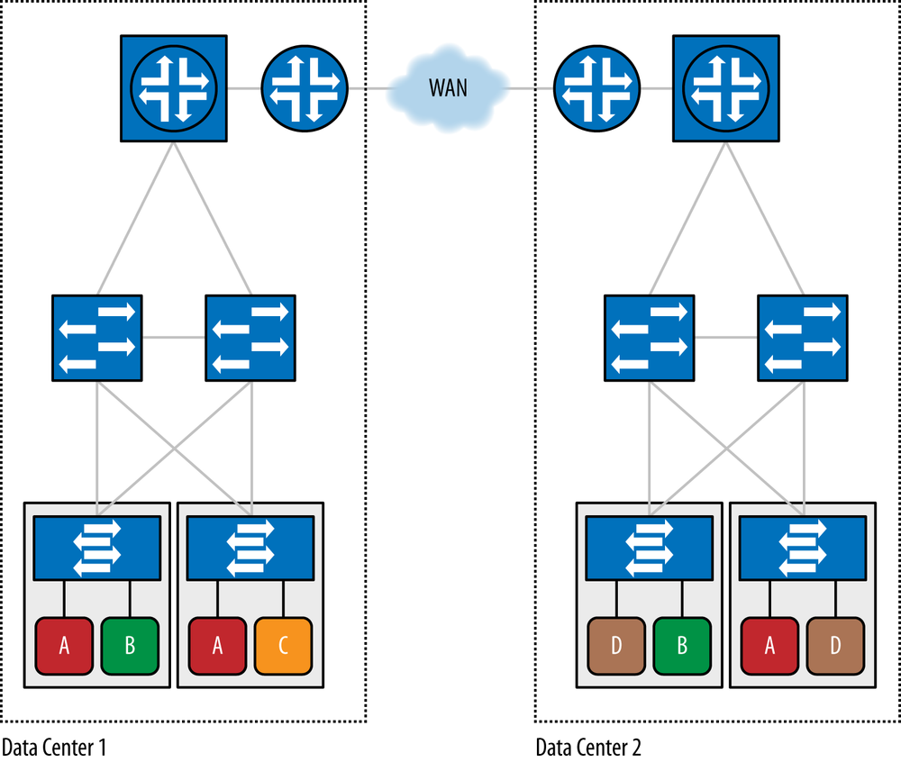
In cases where two or more data centers exist, then you must consider how to connect these data centers. For example, a tenant may have arbitrary numbers of virtual machines residing in each of these different data centers yet desires that they be at least logically connected. The Data Center Interconnect (DCI) (see Figure 6-13) puts all VMs of a given tenant across all data centers on the same L2 or L3 underlying (i.e., underlay) tenant network.[130] It turns out in order to interconnect data centers, you can treat data centers almost like Lego blocks that snap together, using one of the concepts extrapolated from the multitenant data center concept already discussed.
As it turns out, interconnecting data centers is not necessarily a simple thing because there are a variety of concerns to keep in mind. But before jumping feet first into all the various ways in which DCI can be implemented, let’s first examine some of the requirements of any good DCI solution, and more importantly, some of its fallacies.
When designing a data center and an architecture, or strategy, for interconnecting two or more data centers, one inevitably needs to list the requirements of the interconnection. These often start with a variety of assumptions, and we have found that in practice, many of these fall into a category of things that seem to make sense in theory, but in practice are impossible to guarantee or assume. These assumptions include the following:
The network is reliable.
Latency is zero.
Bandwidth is infinite.
The network is secure.
Topology doesn’t change.
There is one administrator.
Transport cost is zero.
The network is homogeneous.
At first, these notions may seem quite reasonable, but in practice they are quite difficult (or impossible) to achieve. For example, the first four points make assumptions about the technology being employed and the equipment that implements it. No equipment is perfect or functions flawlessly, and so it is often a safer bet to assume the opposite of these first points. In terms of points four to six, these fall under administrative or personnel issues. All things equal, once your network is configured, it should continue operating that way until changed. And therein lies the rub: operational configuration errors (i.e., fat-finger errors) can be catastrophic from the perspective of the normal operation of the network and because they can also inadvertently introduce security holes. (There are statistics that have actually shown a reduction in network failures during holiday or vacation periods, when network operations staff is not operating networks.)
It turns out that the DCI must account for the fact that address spaces of tenants can overlap—for example, using L2 MPLS VPNs, L3 MPLS VPNs, GRE tunnels, SSL VPNs, or some other tunneling mechanism to keep the address spaces separate. Depending on the strategy chosen to manage addresses, these might fall into the issues just discussed under DCI fallacies. In particular, assuming that addresses overlap but are protected from one another can quickly unwind if an operational configuration misconfigures a new tenant that unexpectedly can see another tenant’s VMs. So keep in mind that the choice of an addressing scheme goes beyond the obvious choice and should include consideration of operations and management verification and checking schemes.
There are performance criteria for the interconnection, too. Many of the constraints derive from the concept of live migration between data centers (including disk I/O, as previously mentioned), and there is a great deal of debate over whether live migration is really a use case to be considered in Data Center Interconnect design, given the hurdles that must be passed in order for that to function effectively. For example, discussions in the Broadband Forum on the topic of DCI assert that the VMware VMotion solution requires 622 Mbps minimum bandwidth between data centers and recommends less than 5 ms Round Trip Time (RTT) between source and destination servers (see Figure 6-14). This effectively sets physical limits on the distance between servers. In reality, the answer to how much bandwidth you need is derivable based on known data. This data can be generalized, but is determined largely by the tenant service behavior and target constraints. DCI bandwidth is of a particular concern, as it is directly related to the change window duration and the amount of data to replicate. The RTT and thus, distance of data center separation, is also a constraint.[131] While a calculation could optimize for all constraints, the example just cited was for a three-hour change window for a particular data product with the bandwidth of the link set to a fixed value. Of course, these calculations can be performed for an atomic action or the aggregate of all operational actions, which will result in different values.
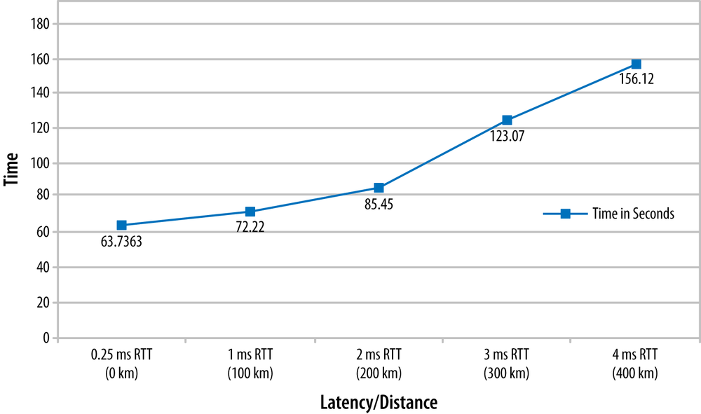
Figure 6-14. Distance limitations for recommended VMotion latency (at interconnect rate of 622 Mbps)
To review, the general scale concerns when designing the DCI include:
MAC address scalability is an issue on the DC WAN edge for solutions that use L2 extension (e.g., 250k client MAC addresses in a single Service Provider data center multiplied across interconnected SP data centers and Enterprise data centers)
Pseudowire scale (i.e., the number of directed LDP sessions, MAC learning)
Control plane scale (i.e., whether or not an L2 control plane domain is extended between data centers)
Broadcast, unknown unicast, and multicast traffic handling (BUM)
In the end, a mixture of layer 2 extensions and IP interconnection may be required. The latter may be straightforward IP forwarding or L3VPN. The outstanding questions are around whether or not the control planes of the different centers are disjoint/separated.
The common approaches for DCI that have been mentioned can be considered across a spectrum starting from the simplest to the most involved, placed into the following categories to better frame their pros and cons:
VLAN Extension uses 802.1q trunking on the links between the data centers and is fraught with the same concerns of VLANs in the data center; MAC scalability, potential spanning tree loops, unpredictable amounts of BUM traffic and little control that allows effective load balancing over multiple links (traffic engineering).
There are some proprietary solutions to the VLAN extension problem. For example, Cisco vPC (virtual port channel) suggests bonding inter-DC links and filtering STP BPDUs to avoid STP looping.
VPLS uses MPLS to create a pseudowire overlay on the physical connection between the data centers. The MPLS requirement comes with an LDP and/or multiprotocol BGP requirement (for the control plane of the overlay) that may (to some operators) mean additional complexity, though this can be mitigated with technique like Auto-Discovery.[132]
MPLS brings additional potentially desirable functionality: traffic engineering, fast reroute, multicast/broadcast replication, a degree of isolation between data centers allowing overlapping VLAN assignments and hiding topology, and fairly broad support and interoperability.
The simplest solution for DCI is to simply use VLANs. In cases where there are fewer than about 4,000 tenants in any given data center, it is perfectly acceptable (and scalable) to use VLANs as a segregation mechanism. This mechanism is supported on most hardware from high-end routing and switching gear, all the way down to commodity switches. The advantages around using this mechanism are that basically they are dead simple to architect and initially inexpensive to operate. The disadvantages are that they are potentially complex to administer changes to later. That is, there are a potentially large number of points that will need VLAN/tag mappings modified in the future if changes are desired.
The VLAN solution for DCs is simply mapped to intra-DC IP or Ethernet paths that carry the tagged traffic between data center gateways, which forward the traffic down to the local data center.
In cases where more than 4,000 tenants are desired, other solutions must be employed. One such option is Virtual Private LAN Service (VPLS). The basic operation of the VPLS solution is similar to that of the VLAN service except that MPLS (L2TPv3) and pseudowires are used to interconnect data centers, and VLANs (or stacked VLANs) are mapped to the pseudowires at the gateways, thus stitching together the data center VLAN-to-VM mappings. This is shown in Figure 6-15 where the CE represents either the gateway router/switch or the top of rack switch (ToR), depending on how far down into the network the architecture requires the VPLS to extend. In the case of the former, the VLAN-to-VPLS tunnel mapping happens at the gateway, while the mapping happens on the ToR in the latter case. Both cases have pros and cons in terms of scale, operations and management, and resilience to change, but in general the VPLS solution has the following characteristics:
Flodding (Broadcast, Multicast, Unknown Unicast)
Dynamic learning of Mac addresses
Split-Horizon and full-mesh of PWs for loop-avoidance in core (no STP runs in the core, so the data center SPT domains are isolated)
Sub-optimal multicast (though the emergence of Label Switched Multicast may provide relief)
The VLAN to pseudowire mapping may place an artificial limit on the number of tenants supported per physical interface (4K)
VLAN-based dual homing may require the use of virtual chassis techniques between the PE/DCI gateways and pseudowire redundancy (for active/active redundancy)
Load balancing across equal cost paths can be only VLAN based (but not flow-based unless we introduce further enhancements like Entropy Labels or Flow Aware Transport (FAT) pseudowires)[133]
While VPLS is an improvement over a simple VLAN or stacked VLAN approach, it does still have issues. For example, the approach is still encumbered by MAC scaling problems[134] due to data plane learning, similar to the VLAN or stacked VLAN approaches. These issues will potentially result in issues at the CE points shown in Figure 6-15. Also, due to having to implement and deploy pseudowire tunnels between the PEs in the network configuration (i.e., either the gateway or the ToR, depending on the architecture) this also adds the potential for pseudowire scale and maintenance issues.
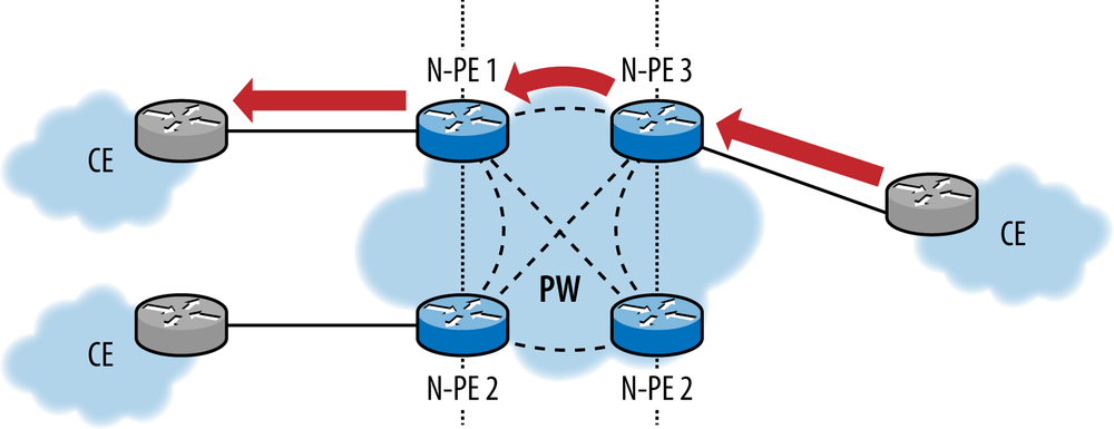
Figure 6-15. VPLS for DCI (split horizon has eliminated the paths to the target CE via N-PE2, NPE-4, and alternate LSPs on N-PE3)
Another MPLS-based solution called Ethernet VPN (EVPN),[135] was developed to address some of the shortcomings of VPLS solutions. EVPN augments the data plane MAC learning paradigm with a control plane solution for automated MAC learning between data centers. EVPN creates a new address family for BGP by converting MAC addresses into routable addresses and then uses this to distribute MAC learning information between PEs in the network. Other optimizations to EVPN have also been made in order to further optimize MAC learning to enhance its scalability.
EVPN can use a number of different transport LSP types (P2P/P2MP/MP2MP)[136] and can provide some distribution advantages over VPLS:
Flow-based load balancing and multipathing (layers 2, 3, and 4) in support of multihoming devices
The same flow-based or VLAN-based load balancing for multihomed networks (this can be based on auto-detection)
Multicast optimization using MP2MP multicast distribution trees
Geo-redundancy for PE/gateway nodes
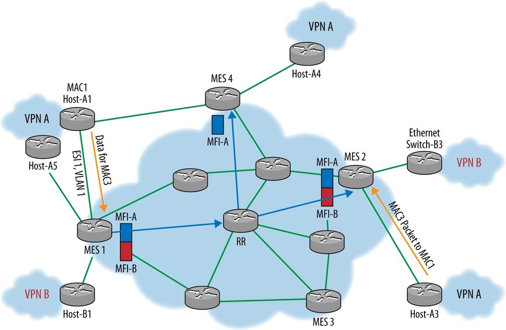
EVPN introduces some new conceptual devices, which are further illustrated in Figure 6-16:
The MES-MPLS Edge Switch
The MFI-EVPN Forwarding Instance
The ESI-Ethernet Segment Identifier (which is important in Link Aggregation scenarios)
Figure 6-16 illustrates how, within the data center, local MAC addresses are still learned through normal data plane learning in the EVPN model. MES(s) can learn local MACs through other mechanisms as well—management plane protocols or extensions to discovery protocols like LLDP—but still distribute these addresses to other PEs using split-horizon and other MAC bridging optimization approaches. The basic operation of EVPN also populates the table for the new address family in the MES and advertises it in BGP updates to neighboring MES(s) in order to distribute MAC routes. Furthermore, a MES injects the BGP learned MAC addresses into their layer 2 forwarding table along with the associated adjacency info. What differs from the typical VLAN approach described earlier is that this now can be done in a far more scalable manner. For example, WAN border routers may forward on the label only, and other MES points may only populate the forwarding plane for active MACs. This differs from having to have each end point learn every MAC address from each VLAN. Effectively, MAC addresses stay aggregated behind each MES much in the way BGP aggregates network addresses behind a network and only distributes reachability to those networks instead of the actual end point addresses.
In addition to these advantages, EVPN does a lot to reduce ARP flooding, which can also lead to scalability issues. ARP storms can consume the forwarding bandwidth of switches very quickly. To this end, the MES performs proxy ARP, responds to ARP requests for IP addresses it represents, and doesn’t forward ARP messages unless the BGP MAC routes carry a binding for the requested IP address.
EVPN also improves MAC learning and selective VLAN distribution through the implementation of BGP policies much in the same way BGP policies are used to enhance normal IP reachability. Route Targets (RTs) are used to define the membership of a EVPN and include MES(s) and Ethernet interfaces/VLANs connecting CEs (e.g., hosts, switches, and routers). RTs can be auto-derived from a VLAN ID, particularly if there is a one-to-one mapping between an EVPN and a VLAN. Each MES learns the ESI membership of all other MES in the VPNs in which it participates. This process enables designated forwarder election and split horizon for BUM traffic (for multihomed CEs).
The example in Figure 6-16 illustrates the capability of EVPN MES(s) to distribute different MFI to other MES that have members of the same VPNs. This is most often implemented employing a route reflector to further enhance scalability of the solution. BGP capabilities such as constrained distribution, Route Reflectors, and inter-AS are reused as well.
Also on Figure 6-16, both MES1 and MES4 advertise Ethernet Tag auto-discovery routes for <ESI1, VLAN1> along with MPLS label and VPNA RT. For example, MES1 advertises MAC Route in BGP:
<RD-1, MAC1, A1-VLAN, A1-ESI ID, MAC lbl L1, VPN A RT>
In the example, MES2 learns via BGP that MAC1 is dual-homed to MES1 and MES4. This still works despite the fact that MES4 might not yet have advertised MAC1 because MES2 knows via the Ethernet Tag auto-discovery routes that MES4 is connected to ESI1 and VLAN1. If MES2 decides to send the packet to MES1, it will use inner label <EVPN label advertised by MES1 for MAC1> and outer encapsulation as <MPLS Label for LSP to MES1> or <IP/GRE header for IP/GRE tunnel to MES1>.
MES2 can now safely load-balance the traffic to MAC1 between MES1 and MES4.
As a summary, we think that it is instructional to compare and contrast the last two solutions for DCI given their similarity. Table 6-1 makes clear that EVPN appears to be the most optimal solution for DCI.
Table 6-1. Summary comparison of VPLS and EVPN for DCI
Desirable 1.2 extension attributes | VPLS | E- VPN |
|---|---|---|
VM Mobility without renumbering L2 and L3 addresses | ✓ | ✓ |
Ability to span VLANs across racks in different locations | ✓ | ✓ |
Scale to few 100K hosts within and across multiple DCs | ✓ | ✓ |
Policy-based flexible L2 topologies similar to L3 VPNs | ✓ | |
Multiple points of attachment with ability to load-balance VLANs across them | ✓ | ✓ |
Active-Active points of attachment with ability to load-balance flows within a single VLAN | ✓ | |
Multi-tenant support (secure isolation, overlapping MAC, IP addresses) | ✓ | ✓ |
Control-Plane Based Learning | ✓ | |
Minimize or eliminate flooding of unknown unicast | ✓ | |
Fast convergence from edge failures based on local repair | ✓ |
In this section we consider SDN solutions for the modern data center. In particular, we will discuss how modern data centers that were just described are having SDN concepts applied to extend and expand their effectiveness, scale, and flexibility in hosting services. We should note that SDN solutions don’t always mean standard solutions, and some of the solutions described are vendor proprietary in some form.
As described earlier, traditional data centers contain storage, compute (i.e., servers), and some network technology that binds these two together. Much in the way that servers and applications have been virtualized, so too have networks. In the traditional network deployment, VLANs were about as virtualized as a network got. In this sense, the VLANs were virtualizing the network paths between VMs. This was the first step in the virtualization of the network. As we introduced earlier in the DCI section, there are a number of protocols that can be used to not only form the network fabric of the data center, but as you will see, that can be used to also virtualize the fabric. In particular, we will introduce the notion of network overlays as a concept that allows for the virtualization of the underlying network fabric, or the network underlay.
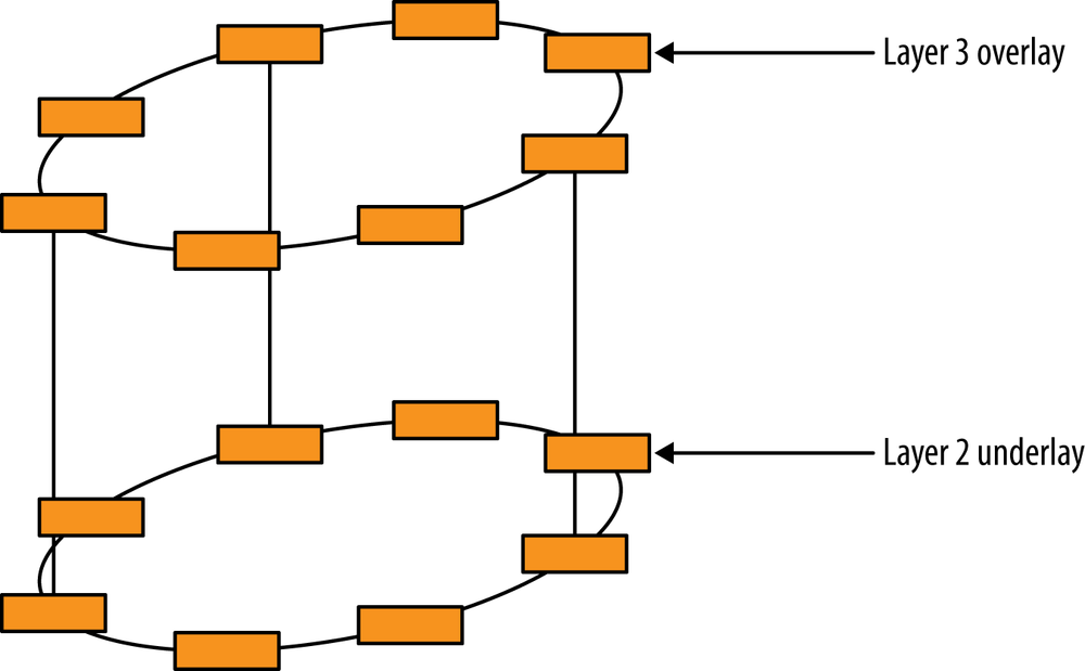
The network underlay can be comprised of a number of technologies. Generally speaking, these can be divided up into layer 1, 2, or 3 solutions, but in all the cases, these solutions are designed to do basically one thing: transport traffic between servers in the data center. Figure 6-17 demonstrates how an overlay network creates a logical network over the physical underlay network. Typically the overlay network is created using virtual network elements such as virtual routers, switches, or logical tunnels. The underlay network is a typical network, such as an Ethernet, MPLS, or IP network.

Frankly speaking, all of the available solutions will work at providing an underlay network that carries an overlay. The question is one of how optimal each solution is at what it does, and how good it is at hosting a particular overlay technology. For example, while one solution might scale better for layer 2 MAC address learning, it may be terrible when one considers how this is used to handle VM moves or external cloud bursting. Another example might scale well for its speed of adapting to changes in the network, while another might require more time for semi-automated (or even manual) operator intervention. We will investigate all of these angles in the following section.
This chapter is squarely focused on new SDN technologies, but do not lose sight that simplicity is king when operating a network. To this end, when tenancy of internal tenants is needed only, and that number does not exceed about 1,000, VLANS are still the simplest and most effective solution. This is a well-known approach, quite easy to operate, and is supported on the widest variety of hardware, so the simplest form of a network overlay is of course a flat IP network that rides over a VLAN substrate or underlay. This is in fact how data centers were originally constructed. There was no real need at the time to support multiple tenants, and when there’s a need to segregate resources based on departmental access, VLANs were invented, but the overlay was still a relatively flatly addressed IP network. This approach even worked for a short while for external user access to data centers (remember the Amazon AWS case) until the number of tenants grew too large, address spaces had to overlap, and the general churn of these virtualized network elements required very fast (re)-programming of these resources. In these scenarios, the basic IP over Ethernet network sufficed for a single tenant and could be easily and unobtrusively extended to support up to about 4,000 tenants using VLANs.
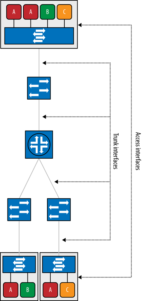
Figure 6-18 illustrates how a basic VLAN approach can be used to implement a localized data center’s overlay along with an IP overlay and implement a relatively simple DC interconnection. In the example, three 801.1q VLANs are created for each application (app, db, and management), and traffic is segregated using these VLANs across the network. In this approach, the same flat IP addressing space is used within the DCs in order to provide layer 3 access to the VMs hosting those services. The interface from the virtual machine to the hypervisor is an access interface. The hypervisor assigns this interface to the VLAN of the tenant. The server-to-access switch interface, as well as all switch-to-switch interfaces, are trunk interfaces.
While VLAN solutions are quite easy to implement, unless routing is inserted between VLANs, it has long been known that relying simply on bridging or the Spanning Tree Protocol (or its variants) does not scale well beyond around 300 hosts on any single VLAN. The problem with the protocol is that when the number of host MAC addresses becomes large, changes, moves or failures result in massive processing inside the network elements. During these highly busy periods, network elements could miss other failures or simply be overloaded to the point where they cannot adjust quickly enough. This can result in network loops or black holes. Early versions of Spanning Tree also suffered from the issue of wasting equal cost (i.e., parallel) links, in that the protocol effectively blocked all parallel links to the same bridge except one as its means of preventing loops. Even the latest versions of these protocols have limited ability to provide multipath capabilities. Finally, in most cases, bridges can suffer from a loss in forwarding of several seconds when they reestablish connectivity to other bridge links.
Earlier we introduced EVPN as a DCI solution, and in doing so noted how the PE function could terminate at the DC gateway or the ToR. In the case of the former, we showed how VLANs (stacked, tagged, or flat) would then be used to form the underlay. We also pointed out that EVPN, as with VPLS, could be used to extend the number of tenants in a network beyond the 4,000 VLAN tag limit.
Figure 6-19 illustrates just how EVPN can be employed within a data center to carry traffic for tenants to other tenants. The general operation is simple in that traffic is transmitted as an MPLS encapsulated frame containing an Ethernet frame. MPLS tunnels terminate at the physical or virtual switch, which then de-capsulates traffic and delivers it as a layer 2 frame to the virtual or physical host, depending on the implementation. Similarly, transmission of layer 2 frames from the end stations are encapsulated into an MPLS tunnel and delivered to other end hosts. This behavior is identical to what was explained earlier.

And Figure 6-20 demonstrates how the control plane establishes a full mesh of transport MPLS LSPs between the access and core switches using LDP or RSVP. The access switches run MP-IBGP to signal MAC learning reachability information in the same way described previously in the DCI section.
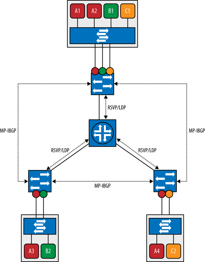
It is important to consider the scaling characteristics of this approach with other methods described earlier. In particular, since the physical network is a layer 3 (MPLS) network, it will scale and be operated in the same well-known ways that MPLS networks are. Similarly, all layer 2 traffic is tunneled across the network over MPLS, which is good for scaling because it avoids having large layer 2 domains and the associated scaling problems with them. Also comparing this approach to VxLAN or NVGRE, one must consider the number of actual tunnels that must be established and managed. In this case, there generally should be fewer than the VxLAN and NVGRE cases because stacked labels can be employed. Further extending the scale of this approach in terms of processing load on the switches is the use of BGP route reflectors in this scheme. These can enhance the solution very much. Finally, use of XMPP between the local switches (or vSwitches) and the MP-IBGP points in the architecture can potentially lighten the protocol configuration load on the end hosts.
The current routing and addressing architecture employed within the Internet relies on a single namespace to express two functions about a network element: its network identity and how it is attached to the network. In essence, the problem is that we want to preserve the device’s identity, regardless of which network or networks to which it is connected. The addressing scheme employed today was invented when network elements were relatively static, and the assumption was that the network-to-element ID binding was relatively static, too. Today we have to consider modern user behavior, where mobile elements rapidly move between base stations or radio access networks. That makes managing network connections, resources, and other things that should be pinned to a network element based on its identifier difficult because its entire address could change when it changes networks. Furthermore, in cases where network elements are multihomed, traffic engineering (TE) is needed, or address allocations are employed that prevent aggregation.
This problem has been exacerbated by two conditions. The first is IPv4 address space depletion, which has led to a finer and finer allocation of the IPv4 addresses space, which results in less aggregation potential. The second is the increasing occurrence of dual-stack routers supporting both IPv4 and IPv6 protocols. IPv6 did not change anything about the use of IP addresses and so still suffers from the same issues that IPv4 does.
A number of people at the IETF recognized these issues and sought to correct them by creating a new address and network element address split called Locator ID Split, or LISP, as it’s now known. They created a network architecture and set of protocols that implemented a new semantic for IP addressing. In essence, LISP creates two namespaces and uses two IP addresses for each network device. The first is an Endpoint Identifier (EID) that is assigned to an end-host and always remains with the host regardless of which network it resides on. The second is a Routing Locator (RLOC) that is assigned to a network device (i.e., a router) that makes up the global routing system. It is the combination of these routers and the unique device identifier and the protocols used to manage them across the Internet that comprise the LISP system and allows it to function.
The separation of device identifier from its network identifier offers several advantages:
Improved routing system scalability by using topologically-aggregated RLOCs.
Improved traffic engineering for cases where multihoming of end-sites are employed.
Provider independence for devices that are assigned an EID from a common EID space. This facilitates IP portability, which is an important feature, too.
LISP is a simple, incremental, network-based implementation that is deployed primarily in network edge devices, therefore requiring no changes to host stacks, Domain Name Services, or the local network infrastructure used to support those hosts.
IP mobility (EIDs can move without changing—only the RLOC changes!)
The concept of a location/ID separation has been under study by the IETF and various universities and researchers for more than 15 years. By splitting the device identity, its Endpoint Identifier, and Routing Locator into two different namespaces, improvements in scalability of the routing system can be achieved through greater aggregation of RLOCs.
LISP applies to data centers by providing the capability to segment traffic with minimal infrastructure impact, but with high scale and global scope. This is in fact a means by which virtualization/multitenancy support can be achieved—much in the way we have described VLANs or VPNs within DCs. This is accomplished when control and data plane traffic are segmented by mapping VRFs to LISP instance IDs, making this overlay solution highly flexible and highly scalable. This also has the potential for inherently low operational cost due to the mapping being done automatically by the DC network switches.
An additional benefit of this approach is that data center VM-Mobility can also provide location flexibility for IP endpoints not only within the data center network, but due to using the IP protocol, also across the Internet. In fact, VM hosts can freely move between data centers employing this scheme because the server identifiers, which are just EIDs, are separated from their location (RLOC) in the same way any other implementation of LISP would be. Thus this solution can bind IP endpoints to virtual machines and deploy them anywhere regardless of their IP addresses. Furthermore, support of VM mobility across data center racks, rows, pds, or even to separate locations is possible. This method can also be used to span organizations, supporting cloud-bursting capabilities of data centers.
Virtual Extensible LAN (VxLAN) is a network virtualization technology that attempts to ameliorate the scalability problems encountered with large cloud computing deployments when using existing VLAN technology. VMware and Cisco originally created VxLAN as a means to solve problems encountered in these environments. Other backers of the technology currently include Juniper Networks, Arista Networks, Broadcom, Citrix, and Red Hat.
VxLAN employs a VLAN-like encapsulation technique to encapsulate MAC-based layer 2 Ethernet frames within layer 3 UDP packets. Using a MAC-in-UDP encapsulation, VxLAN provides a layer 2 abstraction to virtual machines (VMs) that is independent of where they are located for reasons similar to why LISP was invented. Figure 6-21 demonstrates the packet format employed by VxLAN. Note the inner and outer MAC/IP portions that provide the virtual tunneling capabilities of this approach.

As mentioned earlier, the 802.1Q VLAN Identifier space is limited to only 12 bits, or about 4,000 entries. The VxLAN Identifier space is 24 bits, allowing the VxLAN Id space to increase by over 400,000 percent to handle over 16 million unique identifiers. This should provide sufficient room for expansion for years to come. Figure 6-21 also shows that VxLAN employs the Internet Protocol as the transport protocol between VxLAN hosts. It does this for both unicast and multicast operation. The use of IP as the transport is important as it allows the reach of a VxLAN segment to be extended far beyond the typical reach of VLANs using 802.1Q.
Fundamentally, VxLAN disconnects the VMs from their physical networks by allowing VMs to communicate with each other using a transparent overlay that is hosted over physical overlay networks. These overlay networks can also span layer 3 boundaries in order to support intra-DC scenarios. An important advantage to VxLAN is that the endpoint VMs are completely unaware of the physical network constraints because they only see the virtual layer 2 adjacencies. More importantly, this technology provides the capability to extend virtualization across traditional network boundaries in order to support portability and mobility of VM hosts. VxLAN allows for the separation of logical networks from one another much like the VLAN approach could, simplifying the implementation of true multitenancy, but extends it further by also exceeding the 4,000 VLAN limit with a much larger virtualization space.
The normal operation of VxLAN relies on Virtual Tunnel Endpoints (VTEPs) that contain all the functionality needed to provide Ethernet layer 2 services to connected end systems. VTEPs are located at the edges of the network. VTEPs typically connect an access switch to an IP transport network. Note that these switches can be virtual or physical. The general configuration of a VxLAN VTEP is shown in Figure 6-22.
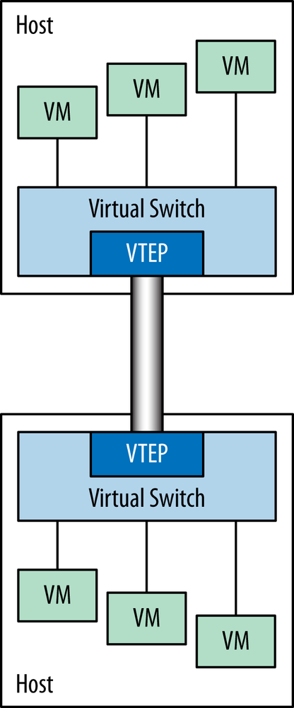
Figure 6-22. VTEP as part of a virtual (or physical) switch connecting VMs together across a data center infrastructure
Each end system connected to the same access switch communicates through the access switch in order to get its packets to other hosts. The access switch behaves in the same way a traditional learning bridge does. Specifically, it will flood packets out all ports except the one it arrived on when it doesn’t know the destination MAC of an incoming packet and only transmits out a specific port when it has learned a forwarding destination’s direction. Broadcast traffic is sent out all ports, as usual, and multicast is handled similarly. The access switch can support multiple bridge domains, which are typically identified as VLANs with an associated VLAN ID that is carried in the 802.1Q header on trunk ports. However, in the case of a VxLAN enabled switch, the bridge domain would instead by associated with a VxLAN ID.
Under normal operation, the VTEP examines the destination MAC address of frames it handles, looking up the IP address of the VTEP for that destination. The MAC-to-OuterIP mapping table is populated by normal L2 bridge learning. When a VM wishes to communicate with another VM, it generally first sends a broadcast ARP, which its VTEP will send to the multicast group for its VNI. All of the other VTEPs will learn the Inner MAC address of the sending VM and Outer IP address of its VTEP from this packet. The destination VM will respond to the ARP via a unicast message back to the sender, which allows the original VTEP to learn the destination mapping as well.
When a MAC address moves to a different physical or virtual switch port (i.e., a VM is moved), the other VTEPs find its new location by employing the same learning process described previously whereby the first packet they see from its new VTEP triggers the learning action.
In terms of programmability, VxLAN excels by providing a single interface to authoritatively program a layer 2 logical network overlay. Within a virtualized environment, VxLAN has been integrated into VMware’s vSphere DVS, vSwitch, and network IO controls to program and control VMs, as well as their associated bandwidth and security attributes.
The Network Virtualization using Generic Routing Encapsulation (NVGRE) protocol is a network virtualization technology that was invented in order to overcome the scalability problems associated with large data center environments that suffer from the issues described earlier in the VLAN underlay option. Similar to VxLAN, it employs a packet tunneling scheme that encapsulates layer 2 information inside of a layer 3 packet. In particular, NVGRE employs the Generic Routing Encapsulation [GRE] to tunnel layer 2 packets over layer 3 networks. At its core, NVGRE is simply an encapsulation of an Ethernet layer 2 Frame that is carried in an IP packet. The result is that this enables the creation of virtualized L2 subnets that can span physical L3 IP networks. The first specification of the protocol was defined in the IETF in draft-sridharan-virtualization-nvgre-00. Its principal backer is Microsoft.
NVGRE enables the connection between two or more L3 networks and makes it appear to end hosts as if they share the same L2 subnet (Figure 6-23). Similarly to VxLAN, this allows inter-VM communications across L3 networks to appear to the end stations as if they were attached to the same L2 subnet. NVGRE is an L2 overlay scheme over an L3 network.
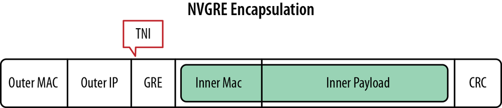
NVGRE uses a unique 24-bit ID called a Tenant Network Identifier (TNI) that is added to the L2 Ethernet frame. The TNI is mapped on top of the lower 24 bits of the GRE Key field. This new 24-bit TNI now enables more than 16 million L2 (logical) networks to operate within the same administrative domain, a scalability improvement of many orders of magnitude over the 4,094 VLAN segment limit discussed before. The L2 frame with GRE encapsulation is then encapsulated with an outer IP header and finally an outer MAC address. A simplified representation of the NVGRE frame format and encapsulation is shown in Figure 6-24.
NVGRE is a tunneling scheme that relies on the GRE routing protocol as defined by RFC 2784 as a basis but extends it as specified in RFC 2890. Each TNI is associated with an individual GRE tunnel and uniquely identifies, as its name suggests, a cloud tenant’s unique virtual subnet. NVGRE thus isn’t a new standard as such, since it uses the already established GRE protocol between hypervisors, but instead is a modification to an existing protocol. This has advantages in terms of operations and management, as well as in terms of understanding the other characterizes of the protocol.
The behavior of a server, switch, or physical NIC that encapsulates VM traffic using the NVGRE protocol is straightforward. For any traffic emanating from a VM, the 24-Bit TNI is added to the frame, and then it is sent through the appropriate GRE tunnel. At the destination, the endpoint de-encapsulates the incoming packet and forwards that to the destination VM as the original Ethernet L2 packet.
The inner IP address is called the Customer Address (CA). The outer IP address is called the Provider Address (PA). When an NVGRE endpoint needs to send a packet to the destination VM, it needs to know the PA of the destination NVGRE endpoint.
We have described a number of underlay approaches that map loosely to variants of existing layer 2 network protocols. The one exception to this is the use of the OpenFlow protocol to establish and manage the underlay network over which, say, an IP network can be overlaid. In Chapter 3 and Chapter 10, we described the protocol’s general operation, and so we will not repeat it here. However, it is useful to show how such an underlay would be constructed, and fortunately, it is quite simple.
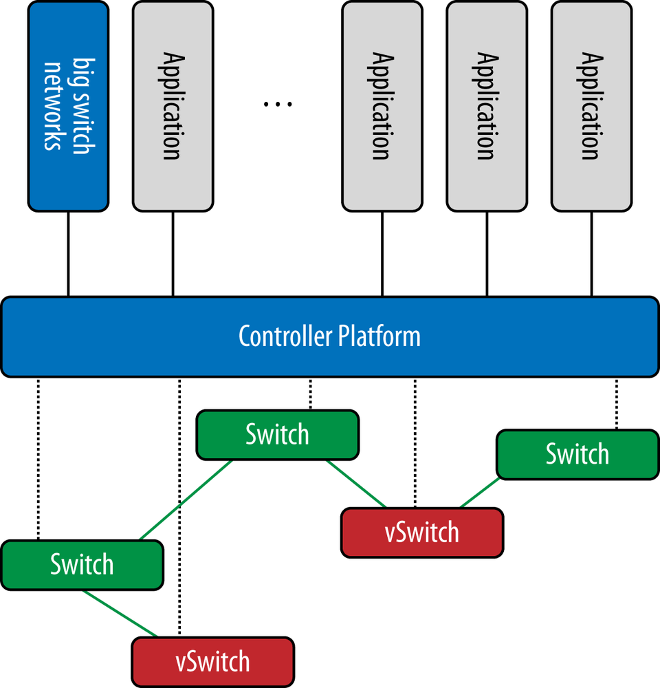
Figure 6-25 demonstrates how an OpenFlow controller is setup in the canonical fashion to control a zone of a network’s switches. Note that while we show the BigSwitch Floodlight controller in the figure, any OpenFlow controller can be swapped into this picture with basically identical operation. The switches in the figure are generally setup to be completely controlled by the controller, although as we described in Chapter 3, the hybrid mode of operation is also a distinct (and practical) possibility here. Each switch has an established control channel between it and the controller over which the OpenFlow protocol discourse takes place. Note that the switches that are controlled are shown as both virtual (vSwitch) and real (switch). It is important to understand that generally speaking, it does not matter whether the switch is virtual or real in this context.
The switches are generally constructed and configured by the controller to establish layer 2 switching paths between the switches, and will also incorporate layer 3 at the ingress and egress points of the network to handle things such as ARP or other layer 3 operations. We should note that it is possible to construct a true combined layer 2 and 3 underlay using this configuration, but the general consensus is that this is too difficult in terms of scale, resilience to failure, and general operational complexity if implemented this way. These issues were discussed in Chapter 4.
As mentioned earlier, while SDN has not invented the notion of logical network overlays, this is clearly one of the things that drives and motivates SDN today, especially in data center networks. Earlier in this chapter, we introduced the notation of a network underlay. The underlay is by and large the network infrastructure technologies employed by data center and other network operators today. With some exceptions, such as VxLAN and NGVRE, these basic technologies have been modified or augmented in order to support additional virtualization, user contexts, or entire virtual slices of the network itself. As with the variety of network underlays, a variety of network overlays exist. We will describe each of these, starting with the general concepts of where tunnels can be terminated that span between virtual machines.
Earlier in Chapter 4, we described virtual swtiches or vSwitches. A number of these exist both in the open source and commercial spaces today. Arguably, the most popular is the Open Virtual Switch, or OVS. We will generally refer to OVS in the rest of this chapter.
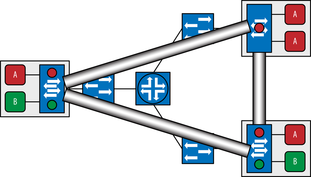
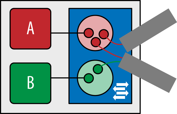
In this class of solution, you establish tunnels between vSwitches to carry the tenant traffic between other vSwitches. Since vSwitches generally reside within the hypervisor space, the vSwitch acts as a local termination and translation point for VMs. It also has the advantage of it not being modified in any way to participate in the overlay (or underlay for that matter). Instead, a VM is presented with an IP and MAC address, as they are in a non-overlay environment and happily exist. There are two subclasses of solutions when terminating tunnels at vSwitches: single and multitiered. The former solution is typical of many of the standards-based solutions that we will get into detail about a little later but generally depict a network comprised of multiple logical and physical tiers that when interconnected, form the underlying infrastructure that the overlay rides over. This approach is demonstrated in the Figure 6-26. In the figure, the VMs are shown as A and B boxes. The letters denote group membership of a particular overlay, or VPN. The larger boxes they reside in represent the physical host machine (server). The rectangle within this box represents the vSwitch. Observe how logical network tunnels are terminated and emanate from this point. This is the case regardless of the underlying network or underlay.
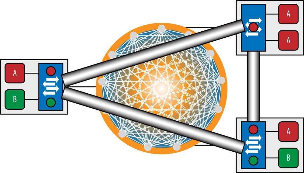
The other approach to overlays is a single-tiered approach. These are generally referred to as data center fabrics and most often are vertically integrated solutions that are largely proprietary, vendor-specific solutions. In these solutions, each overlay tunnel begins and ends in a vSwitch as they did in the multitiered solution, as shown in Figure 6-27. However, it differs from the multitiered solution in that these solutions generally establish a full mesh of tunnels among the vSwitches that establish a logical switching fabric. This potentially makes signaling and operations of this network simpler because the network operator (or their OSS) need not be involved in any special tunnel signaling, movement, or maintenance: instead, the fabric management system takes care of this and simply presents tunnels to the VMs as if they were plugged into a real network.
As mentioned earlier, network overlays exist that emulate different logical layers of the network. These include layers 2 and 3, and more recently one approach that tightly combines layer 1 with layer 2.
It can be argued that the majority of overlay tunneling protocols available encapsulate layer 2 tenant network traffic[137] over some layer 3 networks, although OpenFlow is the obvious variant in this case, where the usual approach is to construct a network out of entire layer 2 segments, as described earlier. The layer 3 network is typically IP, although as we have seen can be OpenFlow, GRE, or even MPLS, which is technically layer 2.5 but is counted here. The exact format of the tunnel header varies depending on the tunneling encapsulation, but the basic idea is approximately[138] the same for all encapsulations, as shown in Figure 6-28.
The focus around layer 2 networking was historically driven by server clustering technologies[139] and storage synchronization, as well as the need for the network operator of OSS to have more freedom in binding IP addresses to VMs. However, these applications are no longer exclusively layer 2; we are seeing more and more migration to layer 3.
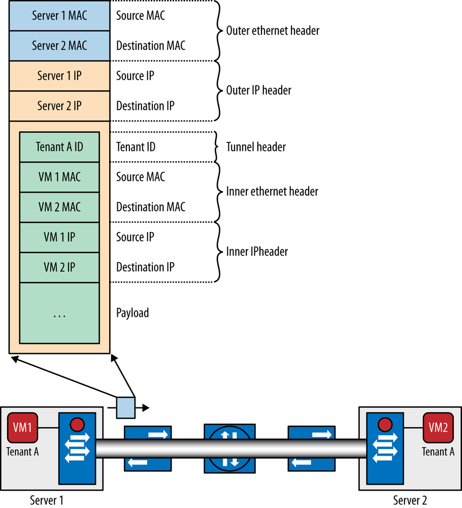
All of the tunnel encapsulation used in these solutions uses some sort of tenant identifier field in the tunnel header to de-multiplex the packets received from the tunnel into the context of the right vswitch bridge, as shown in Figure 6-29:
GRE uses the 32-bit GRE key [GRE-KEY-RFC] (32 bits).
VxLAN uses the 24-bit VxLAN segment ID, also known as the VxLAN Network Identifier (VNI).
NVGRE uses the 24-bit Virtual Subnet ID (VSID), which is part of the GRE key.
VmWare/Nicera’s STT uses the 64-bit Context ID.
MPLS uses the 20-bit inner label.
The VNI in VxLAN, the VSID in NVGRE, and the context ID in STT have global scope across the data center. The inner label in MPLS has local scope within the vswitch, too.
Another type of network overlay are layer 3 (i.e., IP) overlays. These overlays present IP-based overlays instead of layer 2 overlays. The difference between these overlays and layer 2 overlays is that instead of presenting a layer 2 logical topology between VMs, it presents a layer 3 network. The advantages of these approaches are analogous to existing layer 3 VPNs. In particular, private or public addressing can be mixed and matched easily, so things like cloud-bursting or external cloud attachment is easily done. Moves are also arguably easier. In this approach, rather than termination of a layer 2 tunnel at the vSwitch, a layer 3 tunnel is terminated at a vRouter. The vRouter’s responsibilities are similar to those in a vSwitch except that it acts as a Provider Edge (PE) element in a layer 3 VPN. The most typical of these approaches proposed today is in fact a modified layer 3 MPLS approach that integrates with a vRouter inside of the hypervisor space.
One approach that differs from the strictly layer 2 or strictly layer 3 approaches just described is one from a new startup called Plexxi. This solution is an underlay solution but at the same time provides a closely integrated overlay (Figure 6-30). We refer to this as a hybrid overlay-underlay. In the case of overlays, operators must still be conscious of network capacity, as this is a finite resource. Overlays are entirely unaware of the network, and as the entire overlay administrator knows, there is infinite bandwidth supporting them. In traditional network designs, including leaf/spine designs, capacity is statically structured. Studies have shown that much of the capacity in such a network remains idle. Plexxi’s approach is to collapse the data center network into a single tier and to interconnect switches within this tier optically. This results in potentially fewer boxes and far less cabling and transceivers as part of this solution. When combined with dynamically maintained affinities, this means applications can have the capacity they require when they need it without structuring an abundance of otherwise unused capacity ahead of time.
In this approach, overlays are rendered into affinities, allowing capacity in the network to be managed dynamically, even though endpoints are hidden within the overlay. This is possible because the data required to do this is harvested from the overlay management system by a connector, which in turn pushes the data to the Plexxi controller via its API. The Plexxi controller is discussed in detail in Chapter 4, so it is not discussed further here.
In this chapter, we presented a number of concepts and constructs that are used to create, run, maintain, and manage modern multitenant data centers. Some of these concepts are variations on an old theme, while some are new and driven from the SDN movement. In all cases, these solutions provide virtualized network access between virtual machines that wish to communicate privately from the other tenant VMs hosted in a data center operated by a single service provider. In some cases, these technologies can even be used to facilitate VMs that wish to communicate across data centers that span multiple providers. In some cases, the technologies explained allow these logical networks to span multiple data centers owned and operated by the same enterprise, or even multiple enterprises. Later in the book, we will consider some of the design implications of using one technology over another when implementing a data center.
[128] The schema-sharing degree comparison also included a second-degree example (Intaact, which had a 1:250 schema/customer ratio) and a lesser-degree example, which was the Oracle pod architecture (that the author labels “the abandonment of the shared schema principle”).
[129] Alternatives are available that use active/active synchronous data distribution between volumes, where distances supported are claimed to be up to 100 kilometers.
[130] Another layer 2 network driver in Data Center networks is continual connectivity through VM motion. In general, during VM mobility, the source and destination server don’t need to be on the same IP subnet, but to maintain IP connectivity, extending layer 2 connectivity may be attractive.
[131] The RTT/distance relationship is (for the most part) governed by the speed of light in fiber cables, so the 400 kilometer distance limitation comes from a rough calculation using .005ms/km as speed of propagation (and the fact that this is a round trip measurement, so the actual budget is 2.5 ms each way).
[132] RFC 4761 (BGP-Based VPLS), RFC 4762 (LDP-Based VPLS), BGP Autodiscovery for LDP-Based VPLS RFCxxxx, Hierarchical VPLS option for LDP based VPLS
[133] RFC 6790 for Entropy Labels and RFC 6391 for FAT Pseudowires
[134] One proposal to address the MAC issue is to use PBB/802.1ah with VPLS.
[135] EVPN can also be combined with PBB, propagating B-MAC addresses with EVPN. PEs perform PBB functionality just like PBB-VPLS C-MAC learning for traffic received from ACs and C-MAC/B-MAC association for traffic received from the core. Cisco OTV offers some of the characteristics of EVPN but is a Cisco-specific solution.
[136] Because MPLS core networks may be problematic for some, IP/GRE tunnels can also be used to interconnect the MES(s). Fast convergence is based on local repair on MES-CE link failures.
However, in this scenario, in a non-MPLS core, you obviously lose the potential for MPLS Fast Re-Route protection of the tunnels. IP-FRR may, depending on your topology, be an adequate substitute that would require you to run the LSPs over TE tunnels between the MES(s).
[137] The option of tunneling layer 2 over layer 3 tenant network traffic is considered as a separate variation.
[138] When MPLS is used, the outer IP header is replaced by an MPLS header, and the tunnel header is replaced by a stacked MPLS header.
[139] E.g., Microsoft MSCS, Veritas Cluster Server, Solaris Sun Cluster Enterprise, VMware Cluster, Oracle RAC (Real Appl.Cluster), HP MC/ServiceGuard, HP NonStop, HP Open VMS/TruCluster, IBM HACMP, EMS/Legato Automated Availability Manager