In an indirect proof of a statement “A”, it is customary to show that the assumption of “ A” leads to a contradiction, so that “A” must be false and thus “A” is true. A contradiction is understood to be the denial of an axiom or of a previously proved theorem. In addition, any statement known to be false because of its form alone can serve as a contradiction. Perhaps the simplest such form is “RR”, for whatever the truth value taken for “R”, the truth value of “RR” will clearly be “F”. Therefore, any statement in the form “RR” is false, and can serve as the contradiction in an indirect argument.
We shall take as the basic form of indirect proof of “A” any argument that starts from “A” and leads to a statement in the form “RR”. This basic form includes the case where the contradiction is the denial of an axiom or theorem, for if “R” is an axiom say, and the argument leads to “R”, then by conjunctive inference (2.72) it also leads to “RR”.
The basic form of indirect proof is justified by the rule of contrapositive inference (2.77). The argument will establish “A → RR”. Since “RR” is false, “(RR)” is true; so, by contrapositive inference,
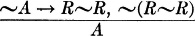
and “A” is proved.
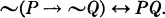
In carrying out an indirect proof, one must be careful to start the argument with the negation of the statement to be proved, or with some statement equivalent to it. In most cases, the statement to be proved is a conditional of the form “P → Q”, so that the argument must start with “(P → Q)”, which is grammatically awkward. Formula (2.41) provides a way out of the grammatical difficulty. Starting with “(P → Q) as minor premise, and “(P → Q) ↔ PQ” as major premise, “PQ” can be inferred by modus ponens. In abbreviated form the inference is described

The indirect argument is completed by showing that “PQ” leads to some contradiction “RR”.
In practice, the use of formula (2.41) and modus ponens is usually tacit, so that the argument appears to start simply from the single statement “PQ”. If we like, we can suppose the argument to start with the two statements “P” and “Q”, since each can be inferred by the inference schemes (conjunctive simplification) (2.73) and (2.74).
As an illustration, suppose that a, b, c are distinct lines in the plane, and we wish to prove the statement
A: If a || c and b || c, then a || b.
Since “A” is in the form of a conditional, we start the indirect proof with
(1) (P → Q): Not; if a || c and b || c, then a || b.
By (3.1),
(2) PQ: a || c and b || c, and a is not parallel to b.
Then, by the inference scheme (conjunctive simplification) (2.73),
(3) P: a || c and b || c;
and in the same way, using (2.74),
(4) Q: a is not parallel to b.
From the definition of parallel lines,

From Steps 4 and 5 by modus ponens,
(6) S: a and b meet at N.
From Steps 3 and 6 by conjunctive inference
(7) PS: a || c and b || c, and a and b meet at N.
From an axiom of geometry we know that there is only one line through a given point parallel to a given line; so we have
(8) (PS): Not; a || c and b || c, and a and b meet at N.
So by conjunctive inference we have reached the contradiction
PS(PS)
so that “(P → Q)”, or “A”, is false, and thus “A” is true.
The conventional language of indirect proofs can be quite misleading. In proofs of the foregoing theorem on parallels, the first statement of the indirect proof is frequently taken to be: “Suppose that a is not parallel to b”. From this it would appear that the indirect proof of “P → Q” starts with “Q”. Of course, if it were possible to show that “Q” leads to a contradiction without using the hypothesis “P”, then “Q” would be proved true. Then if “Q” is true, so is “P → Q” true, as can be seen by consulting the truth table for the conditional (2.3). However, in our proof of the theorem, we used “P” as well as “Q” to arrive at the contradiction “PS(PS)”. It is safe to say that if a theorem is worth stating, then it will not be possible to deduce a contradiction from the denial of its conclusion alone.
Again, the language “suppose a is not parallel to b” may appear to indicate that it is “P → Q” that is to be proved false. Now, “(P → Q) ↔ (P → Q)” is not a valid statement formula, so that this procedure is immediately suspect. Suppose it can be shown that “P → Q” leads to a contradiction. Then “(P → Q)” is proved. This is an awkward form, but it turns out to be equivalent to “PQ”. The equivalence follows from formula (2.41) by replacing “Q” by “Q” and then substituting “Q” for “Q” to obtain
With this formula and modus ponens, “PQ” is proved. Now it is “P → Q” that is supposed to be proved, and instead we have proved “PQ”. To see what has been accomplished by this, it is necessary to look at the relation between these two formulas. From the truth table,
it is easy to see that the following formula is valid:
(3.2) PQ → (P → Q).
[This is formula (2.60).] With “PQ” established, then with (3.2) by modus ponens, “P → Q” can be inferred, and the theorem is proved. The difficulty with this method is that it requires us to prove too much. It can happen that “P → Q” is true when “PQ” is false, and in this case, which is the usual one, the method of proof fails. We say that this is the usual case, because if the stronger statement “PQ” is provable, one would not ordinarily assert the weaker statement “P → Q” as a theorem.
There is a correct way of proving a theorem in the form “P → Q” that starts from “Q”. The method consists in starting from “Q” and deducing “P”. Then “Q → P” is proved and the theorem follows from formula (2.42) by modus ponens. This contrapositive form of proof is neater, and conceptually simpler, than an indirect proof leading to a contradiction, and should be preferred when both methods are available.
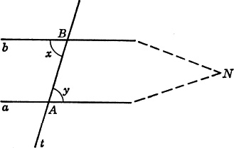
FIG. 6.
The two methods are compared in the following proofs of a standard geometry theorem on parallels cut by a transversal. Suppose lines a and b are cut by a transversal t as in Fig. 6, and it is desired to prove

An indirect proof leading to a contradiction might start with
(1) PQ: (∠x = ∠y)&(a is not parallel to b).
Then by the inference scheme conj simp (2.73),
(2) P: ∠x = ∠y,
and in the same way (2.74),
(3) Q: a is not parallel to b.
From the definition of parallel lines,

By modus ponens, from Steps 3 and 4,
(5) S: a and b meet at N.
Then ABN is a triangle, and we have to suppose that it has already been proved that “an exterior angle of a triangle is greater than either opposite interior angle” so that

Finally, from Step 2 and Step 6 by conjunctive inference,

and a contradiction has been reached.
This proof contains within it the contrapositive form of proof. Steps 3 to 6 give a deduction of “P” from “Q”, that is, they prove “Q → P”, and the theorem “P → Q” follows from the contrapositive equivalence formula (2.42) and modus ponens.
The basic form of indirect proof requires that the argument lead to a contradiction “RR”. In most cases, “R” is an axiom or a previously proved theorem, but occasionally it will be neither of these. It may sometimes be possible to deduce “Q” starting from “PQ”. But “Q” also follows from “PQ” [see (2.74)]; so in this case the contradiction is “QQ” and we have just a special case of the basic form of indirect proof.
As an illustration of this special form of argument, let us prove the following statement in which x stands for some positive real number:

We start the proof from

From Step 1, by conj simp (2.73), it follows that

and also, from (2.74),

From Step 3 it follows that 1/x < 1 so that we may use 1/x for t in Step 2 to obtain

Taking the logarithm of both members, we have

From Step 3 it follows that log x is positive, and so when we divide both sides of the inequality of Step 5 by log x we obtain

and from Step 6, it easily follows that

Finally, from Steps 3 and 7 by conjunctive inference,

and we have the expected contradiction.
It is worth noting that “Q” plays an essential role in this proof in obtaining Step 4 and Step 6.
Sometimes it is possible to start with “PQ” and deduce “P”. Since “P” is also deducible from “PQ” (conj simp), the contradiction in this case is “PP”, and the argument is another special form of the basic indirect argument. This form of argument seems much like the contrapositive argument mentioned at the close of the preceding section. The difference is that in proving “P → Q” by proving “Q → P”, it must be possible to find an argument that leads from “Q” to “P”, which does not need “P” as a step, whereas in the argument leading from “PQ” to “P”, it is necessary to use “P” as a step.
The hypotheses of theorems of geometry and algebra are very often conjunctions. If a theorem has the form “ABC → Q”, then it may be possible to show that “ABCQ” leads to “A” (or “B” or “C”). The required contradiction will then be “AA” (or “BB” or “CC”, respectively).
As an example of proving a theorem of the form “AB → Q” by this method, we prove: “The sum of a rational number and an irrational number is irrational”. That is,
AB → Q: (x rational)(y irrational) → (x + y irrational).
We start the proof by assuming
(1) ABQ: (x rational)(y irrational)(x + y irrational).
As in previous illustrations, we have the steps:
(2) A: x rational (by conj simp)
(3) B: y irrational (by conj simp)
(4) Q: (x + y irrational),
or what is the same,
x + y rational (by conj simp).
Now,
(x + y) — x = y
is true because it is an instance of an algebraic identity. Furthermore, it is known that the difference of two rational numbers is rational; so by Steps 2 and 4, (x + y) — x is rational, and thus y is rational. That is,
(5) B: (y irrational).
By conjunctive inference (Steps 3 and 5) we have “BB”; hence, a contradiction, and the theorem is true.
The form of proof that we have called the basic form of indirect proof is used a great deal in elementary mathematics. In order that the notion of this form of indirect proof be clear, we summarize the format for such proof as follows:
a. The basic form of the indirect proof of a statement “A” is an argument that starts from “A” and leads to a contradiction “RR”.
b. If “A” is a conditional “P → Q”, then the argument can start from “PQ”.
c. If “A” is a conditional “P → Q”, a contradiction can be reached if the argument leads to:
1. The denial of an axiom
2. The denial of a previously proved theorem
3. “Q”
4. “P”
The so-called “proof by the process of elimination” can be the cause of considerable bewilderment to the beginning mathematics student. The method is essentially indirect, and indeed is often presented in elementary geometry textbooks as the fundamental pattern for indirect proofs.
The following recipe for carrying out such proofs, while not a direct quotation, is a fair paraphrasing of such recipes as they occur in several current geometry textbooks.
To prove a theorem by the process of elimination:
a. State the conclusion and all the other possibilities.
b. Show that the other possibilities each leads to a contradiction of the hypothesis or of a truth previously learned.
c. The conclusion is the only remaining possibility.
This apparently explicit set of directions is really quite loose and incomplete. Suppose that the theorem to be proved is a statement of the form “P → A”. For the moment, assume that the first statement of the recipe is understood and that there is just one other possibility “B”. Following the second directive of the recipe, one goes on to show that “B” leads to some contradiction; hence “B” is false and “B” is true. Then according to the third directive, “A” is the only other possibility. However, the goal is to prove “P → A”, and it is not yet clear how this has been done. To clear up this point, it is necessary to investigate what is meant by the phrase “ … all the other possibilities” in the first statement of the recipe.
The phrase “ … all the other possibilities” can be interpreted as meaning a set of alternatives to “A”, that is, a set of additional statements “B”, “C”, …, “F”, such that “P → A∨B∨C∨ … ∨F” is known to be true. With this interpretation, to say that there is just one alternative to “A” is to say that “P → A∨B” is known to be true. Let us examine this case of just one alternative “B” to “A”. Now, “B” is established by showing that “B” leads to some contradiction. If we interpret the third statement of the recipe to mean that now “P → A” is proved, we are asserting that the inference scheme
is correct. It is correct, by mod pon and (2.52), but is not a very practical way of eliminating “B”, because it is hardly ever possible to reach a contradiction from “B” alone without making use of the hypothesis “P”. But if “P” is used, the elimination argument actually starts from “PB”, so that if a contradiction is reached, it is “(PB)” which is established. The inference scheme that must be verified in this case is
The inference scheme (3.3) can be derived from the valid formulas (2.58) and (2.53), which we restate for convenience:
By substituting the first of these into the second, we obtain

Now the inference scheme (3.3) can be verified, for from “P → A∨B” and (3.4) we get

by modus ponens. Then from “(PB)” and (3.5) by modus ponens we get

In some cases it will be possible to eliminate “B” by showing that it leads to “P”, thus proving “B → P”. Since “(B → P) ↔ (P → B)” is an instance of contrapositive equivalence, and since “(PB) ↔ (P → B)” has already been proved valid, it is easy to see that this type of elimination is also justified by the inference scheme (3.3).
To summarize, if “P → A∨B” is known to be true, then if “PB” leads to a contradiction (which may be “PP”), or if “B” leads to “P”, the proof of “P → A” is established. We take this as the basic form of elimination argument. To generalize to the case where there is more than one alternative to “A” is not difficult. The case of just two alternatives should be sufficient for illustration.
Suppose that “P → A∨C∨D” is known to be true. Then “P → A” will be proved if it can be shown that both “PC” and “PD” lead to contradictions. For then, “(PC)” and “(PD)” are established so that, by conjunctive inference, we have “(PC)(PD)”. Now, by replacement in the De Morgan formula (2.39),

and by substitution using the distributive law (2.48),

Then, by substitution,

To justify the outlined elimination procedure, we must verify the inference scheme

But (3.6) is just (3.3) with the placeholder “B” replaced by “C∨D”, so the justification is completed.
As an illustration of a proof by elimination of two alternatives, consider the familiar plane geometry theorem:
In a given circle, if chord AB is greater than chord CD, then chord AB is closer to the center than chord CD.
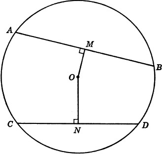
FIG. 7.
In terms of Fig. 7 as lettered, the statement to be proved may be written

Here the disjunction of alternatives may be taken as

Observe that in (3.7),
that is,

Thus, (3.7) can be written as “A∨A”, which is in the form of a valid formula and is therefore a true statement. Since (3.7) is true, then by the definition of the conditional,

is true. The proof may be completed by eliminating the two alternatives as outlined in the previous discussion. Briefly, “PB → P” because by a previously proved theorem, “(OM = ON) → (AB = CD)”.
The contradiction in this case will be “PP”. Also, “PC → P”, because we suppose it has already been proved that “(OM > ON) → (AB < CD)”. Again the contradiction is “PP”. We could also have achieved the eliminations here by proving “B → P” and “C → P”.
The reasoning that assured us of the truth of “P → A∨B∨C” in the foregoing illustration is typical of elimination proofs. In the general case of several alternatives,  is most often known to be true because
  has the special form “A∨A”, that is,

Commonly, “A” and its various alternatives have the property that no two of them can both be true. This is the case in (3.7) of the illustration, but such a property is not a requirement for a proof in this form. For instance, it is known of the decimal representation of any real number x that

The first two statements in (3.8) are not exclusive, for 0.2 and 0.1999 … are decimal representations of the same rational number 2/10, although the first terminates and the second is periodic. If it is desired to prove some real number is irrational, given some facts about its decimal representation, then (3.8) could serve as the disjunction of alternatives in a proof by elimination.
The recipe for proof by elimination, mentioned at the beginning of this section, can be restated with more precision as follows:
To prove “P → A” indirectly by elimination:
a. State enough alternatives “B”, “C”, …, “F” to “A” so that either  is known to be true.
b. Eliminate “F” by showing that “F → P” or that “PF” leads to a contradiction “RR”.
c. If all the other alternatives to “A” are eliminated similarly, then “P → A” is proved.
We have analyzed this type of argument at some length because it is so often treated in elementary textbooks as the general pattern for all indirect proofs. However, it is not so simple as the form we have presented as the basic form of indirect proof, and it is surely harder to describe. If “P → Q” can be proved by showing that “PQ” leads to a contradiction, or by proving the contrapositive “Q → P”, it seems ridiculous to go through the ritual of saying, “Either ‘Q’ is true, or it is false”, in order to cast the argument into the more complex form of a proof by elimination.
EXERCISES
1. Prove: If two chords in a circle are unequal, then their arcs are unequal.
2. Prove: If two sides of triangle ABC are unequal, then the angles opposite these sides are unequal.
3. Prove: If a point is not on the bisector of an angle, then it is not equidistant from the sides of the angle.
4. Prove:  is not rational.
5. Prove:  is not rational.
6. Prove: The product of a nonzero rational number and an irrational number is irrational.
7. Prove: There is no largest prime number.
8. Prove: If x is a positive real number less than 1 such that in its decimal representation, the nth decimal place is occupied by the digit 1 when n is a power of 2, and otherwise the nth decimal place is occupied by a digit different from 1, then x is irrational. Use (3.8).
9. Read the presentations of indirect proof in two different plane geometry textbooks and analyze the descriptions in view of the discussions in Sec. 3.2 and 3.3.
10. Analyze three examples of the use of indirect proof in elementary mathematics.
In proving the plane geometry theorem:
An angle inscribed in a circle is equal in
degrees to one-half of its intercepted arc,
it is customary to break the proof up into three cases, corresponding to the three diagrams of Fig. 8. To analyze the proof by cases formally, let us take as translations:
P: x is inscribed in circle O.
A: x inscribed in O has one side through the center.
B: x inscribed in O has its sides on opposite sides of the center.
C: x inscribed in O has both its sides on the same side of the center.
Q: x is equal in degrees to one-half of its intercepted arc on circle O.
With these translations, the theorem to be proved is “P → Q”. Its proof is established by proving the three cases:

Informally, the idea here is, given “P”, then at least one of the statements “A” or “B” or “C” is true, and since each of them implies “Q” then “P → Q”. The validity of the procedure depends on the correctness of two steps. First, it is necessary to describe the cases so that we know
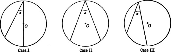
FIG. 8.
and second, the inference scheme,

must be verifiable. To verify the inference scheme, we start with

and infer

by successive applications of conjunctive inference. Next, we need to know that the following formula is valid:

Formula (3.11) can be obtained from (2.54) by substitution and replacement, or may be proved valid by truth tables. Then, from (3.10) and (3.11), by modus ponens, we infer
The inference scheme (3.9) summarizes this sequence of inferences.
Once “P → A∨B∨C” and “A∨B∨C → Q” have been established, “P → Q” can be inferred by the hypothetical syllogism (2.75).
It usually happens in a proof by cases that the hypothesis “P” of the theorem to be proved not only implies, but is equivalent to, the disjunction of the hypotheses in the cases. This is the situation in the foregoing illustration where for “P → A∨B∨C” we could have taken “P ↔ A∨B∨C”. It is also frequently the case that the disjunction of hypotheses is exclusive, but this is not necessary to the validity of the outlined procedure.
Little is said about the method of proof by cases in most geometry textbooks. It is not used with very many theorems, and when it does occur, it is generally accepted by students as a natural way of proving theorems. The method might well be used more freely in geometry. Its use, in conjunction with contrapositive forms of proof, and the basic indirect form, can replace all indirect proofs by elimination.
Consider how the illustration of Sec. 3.3 can be handled as a proof by cases. Recall that in terms of the notation of Fig. 7, the theorem to be proved is

As before, it is assumed known from previous theorems that

and

The theorem can be proved by proving its contrapositive

Since “OM  ON” is the same as “(OM = ON)∨(OM > ON)”, the contrapositive can be proved by the cases:

The form of proof by using the contrapositive and cases seems to us simpler in conception than the proof of the same theorem by the method of elimination of Sec. 3.3.
It is worth noticing that in a proof by cases, there is no requirement that all the cases be proved with the same method. In the foregoing proof, a direct proof is simplest for both cases, but for other theorems it may turn out to be simpler if some of the cases are proved directly and some indirectly.
In summary, where an indirect proof seems indicated there are three main procedures to consider. These procedures are adequate for elementary mathematics, and appear to us to be the simplest possible. To prove a theorem in the form “P → Q”:
a. By a contrapositive method
Prove “Q → P” instead. When this is possible, it seems the neatest of the three procedures.
b. By proving the contrapositive by cases
If in the contrapositive “Q → P”, “Q” is easily expressed as a disjunction “A∨B∨ … ∨F”, then prove the cases, “A → P”, “B → P”, …, “F → P”. Remember that any legitimate method can be used to prove the cases. Some of the cases may be proved indirectly and some directly.
c. By the basic indirect form
Assume “PQ” and deduce a contradiction “RR”. Remember that the contradiction can be “PP” or “QQ”.
EXERCISES
1. Assume it has been proved that:
If two sides of a triangle are unequal, then the angle opposite the longer side is larger than the angle opposite the shorter side.
State a converse and prove it by cases.
2. Assume it has been proved that:
If two triangles have two sides of one equal, respectively, to two sides of the other and the included angle of the first is greater than the included angle of the second, then the third side of the first is greater than the third side of the second.
State a converse, and prove it by cases.
3. Look up the proof of the law of cosines in some standard trigonometry textbook. Analyze the proof in view of the discussion in Sec. 3.4.
4. Repeat Exercise 3 for the proof of the formula for sin ( +
+  ).
).
5. State a converse of the illustrative example of Sec. 3.3, and prove it by cases.
In contrast to the notion of conversion in Aristotelian logic, the formal notion of converse theorem, as used in modern mathematics, is not clearly defined. The converse of “P → Q”, where “P” and “Q” are simple enough statements, is commonly taken to be “Q → P”. For complicated statements there is no general agreement as to the proper way to form the converse. The various ways of forming converses do have in common some sort of interchange of statements between the antecedent and consequent of a conditional.
Elementary mathematics textbooks vary in treatment of conversion. Some simply describe the converse of a theorem as formed by “interchanging the hypothesis and the conclusion”. This is hardly adequate, since few theorems of geometry are actually converted in this way. Others discuss the notion that a theorem may have several related statements that are in some sense its converses. These are distinguished as complete converses and partial converses.
Statements that can be put in the form “P → (Q → R)” are common in elementary mathematics. Should the converse be taken as “(Q → R) → P”, or as “P → (R → Q)”, or perhaps as “(R → Q) → P”? Examples of at least the first two forms occur in both elementary and higher mathematics.
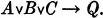
As an instance of the form “P → (Q → R)”, let us state a theorem of plane geometry about a triangle ABC, where the letter m denotes a line.

Possible converses of (3.14) might be taken as
In an attempt to select one of these as the proper converse, one might argue that in (3.14) the implication symbol immediately following “P” indicates the main implication so that the proper choice for the converse should be (3.15). If there is a way of locating the main implication in a statement, then conversion of the statement might be carried out by interchanging the antecedent and consequent of the main implication. Unfortunately, to define the operation of conversion in this way is not quite satisfactory, for it can happen that two equivalent statements have non-equivalent converses. For instance, the validity of the following formula (2.55) was proved as an exercise in Sec. 2.9.

But the formula

is not valid. (Take for “P”, “Q”, “R” the values “T”, “F”, “T”, respectively.)1
Conversion may be thought of as an operation that yields new statements from given conditional statements. As currently used, the operation certainly need not yield true statements when applied to true statements, and when the operation is applied to equivalent statements, it need not even yield equivalent statements. An operation having such properties is not a very useful tool in formal logic.
To gain deeper insight into the meaning of a theorem, it is valuable to consider formally related statements that may be proved, or disproved, as theorems. The statements (3.15) to (3.17) are all conditionals formally related to (3.14) in the sense that they are formed out of substatements contained in (3.14). Proof or disproof of any of them will surely shed light on the properties of isosceles triangles. Perhaps it is this activity of investigating statements related to a proved theorem that is important in elementary mathematics, and this may be carried on without attempting a precise formal definition of conversion. The phrase “a converse” might be used to indicate any statement derived from a theorem by interchanging some statements in its hypothesis with some statements in its conclusion. Certainly the phrase “the converse” is ambiguous as used in most elementary textbooks.
1 It is worth noting that neither of the other forms, (3.16) or (3.17), is equivalent to “R → PQ”.
A basic deductive unit of Aristotelian logic is the syllogism, which was discussed briefly in Sec. 1.2. Recall that the syllogism is a form of argument dealing with four kinds of quantified statements called the A, E, I, O propositions, as in the following examples:
A. All soldiers are volunteers.
E. No soldiers are volunteers.
I. Some soldiers are volunteers.
O. Some soldiers are not volunteers.
These four quantified statements express various degrees of relationship between the classes “soldiers” and “volunteers”. We list them again with the variables “s” and “p” representing placeholders for class names:
A. All s is p.
E. No s is p.
I. Some s is p.
O. Some s is not p.
There is a large, but finite, number of forms of the syllogism that can be constructed using various combinations of the categorical propositions. In classical logic, precise rules are given for determining the 19 forms representing valid forms of reasoning.
Certain immediate forms of reasoning allow conclusions to be drawn from a single proposition as premise. It is clear that A and O propositions with the same class names are opposite in truth value, so that if we know, for instance, that
All soldiers are volunteers
is a true (false) statement, then we know that
Some soldiers are not volunteers
is a false (true) statement. In the same way, the E and I propositions are opposite in truth value, so that the truth of one determines the truth of the other.
Other immediate forms of reasoning were supposed to exist in classical logic. For instance, it was held that the A proposition implies the I proposition having the same class names. So that from
All pigeons are birds
could be inferred
Some pigeons are birds.
The operation of conversion was defined in such a way that the converse of a true proposition was supposed to be true. In the case of an E or an I proposition, the converse was formed by simply interchanging the class names. Thus the E propositions
No American is a traitor.
No traitor is an American.
would be considered mutually converse, as would be the I propositions
Some algebraic numbers are irrational numbers.
Some irrational numbers are algebraic numbers.
In the case of a true A proposition, simple interchange of the class names will not necessarily yield a true proposition. In this case, conversion required a change of quantification as well as an interchange of class names. In classical conversion, the A proposition
All pigeons are birds
becomes the I proposition
Some birds are pigeons.
This type of conversion was called conversion per accidens, and it was supposed that the A proposition implied its I converse. Conversion was not allowed in the case of the O proposition.
We may summarize the Aristotelian conversion rules in the following table:
|
Proposition |
Converse |
|
A. All s is p. |
I. Some p is s. |
|
E. No s is p. |
E. No p is s. |
|
I. Some s is p. |
I. Some p is s. |
|
O. Some s is not p. |
No converse. |
It was supposed that with these rules of conversion, a proposition implies its converse. This property of the operation makes it a useful tool in classical logic.
However, it must be observed that it is a tacit assumption of Aristotelian logic that every class mentioned in a categorical proposition is nonempty. Thus the proposition
All unicorns are four-legged
is not allowed if the class of unicorns is considered to be empty. Or put another way, if the proposition is asserted, it is understood that the class of unicorns (and therefore also the class of four-legged things) has at least one member. For mathematics it is found desirable to use a logic that allows statements about empty classes. It is desirable, so to speak, that the logic take empty classes in its stride. The modern tendency is to take the universal A and E propositions as statements having no existential import and to take the particular I and O propositions as assertions of existence. Thus the statement
All unicorns are four-legged
is allowed, and it is understood that nothing has been asserted about the existence or nonexistence of unicorns or of four-legged things. However, if the class “unicorns” is known to be empty, the statement is considered to be true. On the other hand, the statement
Some unicorns are four-legged
is taken as an assertion of existence, and is considered false if there are no unicorns at all, or if there are no four-legged things.
The statement
All unicorns are four-legged
may be paraphrased as a conditional,
For any thing, if it is a unicorn,
then it is four-legged.
In the paraphrase, the two occurrences of the pronoun “it” clearly refer to the word “thing”. We may rewrite the paraphrase
(3.18) For any x, if x is a unicorn, then x is four-legged.
Now if there are indeed no unicorns, then for every x, “x is a unicorn” is false. But then (3.18) is true in accordance with the definition of “P → Q”. Thus, taking the statement
All unicorns are four-legged
to be true when the class “unicorns” is empty is quite in accord with our notion of the conditional. Conversion per accidens of this statement yields
Some four-legged things are unicorns.
Then if this statement is taken to mean that there is at least one four-legged thing that is a unicorn, and if the class “unicorns” is indeed empty, the statement must be considered false. It follows that conversion per accidens does not always yield a true converse from a true statement when empty classes are permitted.
These difficulties can be avoided by ruling out of the logic all statements about empty classes, but particularly for mathematics it is much more desirable to alter the logic in such a way that empty classes can be treated on the same footing as nonempty classes. In such a logic, the Aristotelian notion of conversion has to be dropped. In modern mathematics, the term “converse” is generally applied only to conditionals, and although the term may be loosely used, mathematicians unanimously agree that the converse of a true conditional need not be true.
The term “inverse” or “inverse theorem” occurs in some plane geometry textbooks. By the inverse of a theorem in the form “P → Q” is meant a conditional of the form “P → Q”. The word “inverse” is used in a variety of ways in higher mathematics, but virtually never in the above sense.
Considered as a formal operation, “inversion” is about as unsatisfactory as the operation “conversion”. The inverse of a true conditional is not necessarily true (or necessarily false), and inverses of equivalent conditionals need not be equivalent. For example, as has been already verified,

is a valid formula, but for the inverses,

is not a valid formula, as may be verified by truth tables.
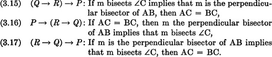
The relationship between a theorem and its contrapositive, converse, and inverse is frequently displayed in the diagram
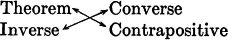
in which the double-headed arrows are supposed to indicate equivalence. For a theorem in the form “P → Q”, the diagram may be given
This type of diagram is apt to appear in the discussion of “locus” in plane geometry, where it is necessary to prove theorems of the form “P ↔ Q”. It is pointed out that in order to prove equivalence, it is sufficient to prove any pair of statements in the diagram not diagonally opposite one another. Either diagram, and discussion of it, is designed to teach greater flexibility in handling theorems of the “if and only if” type, which always state an equivalence.
There is nothing about the diagrams and the rule for their use that would not already be known to a student who understands contrapositive equivalence. It seems more direct to point out that “P ↔ Q” can be proved by proving both “P → Q” and “Q → P”, and to remind the student that it may be easier to prove “P → Q” by proving its contrapositive “Q → P” instead, and similarly, it may be easier to prove “Q → P” by proving “P → Q”. Nothing would be gained here by introducing the notion of “inverse”. Even less would be gained by using “inverse of the converse” in place of “contrapositive” as some authors do.
As an example, consider the standard locus theorem:
The locus of a point X that is equidistant from two given points A and B is the perpendicular bisector m of the segment AB.
To prove this, it is necessary to prove the two statements:

If it is easier to prove (3.19) by proving its contrapositive, then one would prove

and if it is easier to prove (3.20) by proving its contrapositive, then one would prove

Finally, it might be that the basic indirect form of proof is the easiest way of proving (3.19) or (3.20).
EXERCISES
For each locus theorem (in the plane), write out statements in the forms “P → Q” and “Q → P” whose proofs will constitute a proof of the theorem. Write out the corresponding contrapositives, and decide which pair of the four statements you have written you would choose to prove. Consider the case for an indirect proof in Exercises 1 and 2.
1. The locus of a point equidistant from the sides of an angle is the bisector of the angle.
2. The locus of the vertex of an isosceles triangle with a given base is the perpendicular bisector of the base.
3. The locus of a point equidistant from two intersecting lines a and b is two lines that bisect the angles formed by a and b.
4. The locus of the vertex of the right angle of a right triangle having a given hypotenuse is a circle whose diameter is the given hypotenuse. (Strictly speaking, the end points of the hypotenuse are not part of the locus.)
5. The equation of the locus of a point at distance r from the origin is x2 + y2 = r2.
6. The equation of the locus of a point such that the sum of its distances from (—c,0) and (c,0) is 2a, where c2 = a2 — b2 and a > c, is x2/a2 + y2/b2 = 1.
7. Verify that to prove a statement of the form “P → (Q ↔ R)”, it is sufficient to prove “P → (Q → R)” and “P → (R → Q)”. Consider contrapositive variations of these statements.
8. Can you infer “P → (Q → R)” from “PQ → R” and “PR → Q”?
9. What statements would you prove to establish the theorem:
If ABC is a triangle, then AC = BC if and only if ∠A = ∠B.
10. What statements would you prove to establish the theorem:
If a and b are real numbers, then ab = 0 if and only if a = 0 or b = 0.
Up to this point, only short arguments have been considered. We have considered what might be called “units of deduction”. Some abbreviated demonstrations have been presented, and proof has been discussed informally without any attempt at precise definitions of these notions.
In this section, a formal criterion is provided for accepting or rejecting any string of statements offered as proof of a theorem.
A theorem of plane geometry is a statement within the geometry (i.e., a statement about points, lines, planes, distance, etc.) that follows from the basic geometric axioms. To decide whether or not a statement is a theorem, one tries to construct a demonstration that the statement does indeed follow from the axioms, or tries to construct a demonstration that the denial of the statement follows from the axioms.
In attempting to discover statements that are likely candidates for theorems, every available means is employed, including considerations of meaning and form. Successful discovery is generally the result of experience, hard work, and luck. When a likely candidate for a theorem is discovered, construction of its demonstration is also aided by considerations of meaning. But the demonstration itself is the expression of a formal argument, and its validity depends solely on its form. The definition of a demonstration given in the next paragraph is couched in terms of form alone, and the task of checking a demonstration for validity is just a mechanical process of checking the form of each statement in it against this definition.
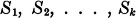
A demonstration that a statement “P” follows as a consequence of statements “A1, A2, …, An” is a sequence of statements “S1, S2, …, Sk” where “Sk” is the same as “P”, and for each “Si” in the sequence, one of the following is the case:
D1: “Si” is one of the statements “A1, A2, …, An”.
D2: “Si” is in the form of a valid statement formula.
D3: “Si” follows from earlier statements in the sequence by means of an established inference rule.
D4: “Si” is the same as some earlier statement in the sequence.
We express the notion that there is a demonstration that “P” follows from “A1, A2, …, An” by writing

The symbol  is called a turnstile, and the statement (3.21) is usually read, “A1, …, An yields P”.1
The condition D4 is included in the definition for convenience, but it is not essential. It permits repetition of statements in a demonstration, but for every demonstration of (3.21) having repetitions, there exists one not having repetitions. To see this, consider a demonstration, “S1, S2, …, Sk” in which “Sj” is the same as an earlier statement “Si”. Then if “Sj” is deleted from the sequence, the remaining k — 1 statements still satisfy the definition of a demonstration. In this manner, all repetitions may be eliminated to obtain a demonstration in which all the statements are distinct and satisfy the conditions D1, D2, D3. Of course, it is a requirement that the last statement “Sk” be the statement we want to demonstrate. What happens if in the process of deleting redundancies, we delete “Sk”? Clearly, we may delete “Sk” only if it is the same as some earlier statement, say “Sr”. But in this case, “S1, S2, …, Sr” is already a demonstration, and the statements “Sr + 1, …, Sk” are redundant in the demonstration and may all be deleted.
A useful property of  may be stated

To see this, suppose
is a demonstration of “P Q” and that

is a demonstration of “Q R”. Then it turns out that,

is a demonstration of “P R”. To verify this, we have to check the sequence against the definition of a demonstration. Clearly, “Sr*” is the same as “R” and the “Si” for i = 1, …, k satisfy the definition. There is no difficulty about any “Sj*” which comes under one of the cases D2, D3, or D4 in (3.23), because it will come under the same case in (3.24). But if “Sj*” comes under D1 in the sequence (3.23), then “Sj*” is the same as “Q”, and this “Sj*” cannot come under the case D1 in the sequence (3.24). However, we know that “Sk” is the same statement as “Q”, so that in (3.24), “Sj*” is just a repetition of “Sk” and thus comes under case D4.
The preceding argument can be extended to justify the following generalization of (3.22):
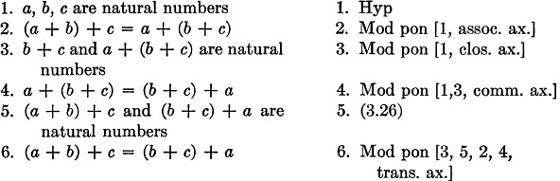
The following illustrative demonstration is based on an axiom for natural numbers called the “Closure Axiom”. In the demonstration, we have to use statements of the form “x is a natural number” so often that it is useful to have an abbreviation. For “x is a natural number” we shall write “x ε N”. Here “N” stands for the class of natural numbers, and “ε” is read “is an element of” or “is a member of”.
The Closure Axiom for natural numbers is

We wish to exhibit a demonstration proving

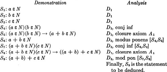
The column headed Analysis is not a part of the demonstration, but should be regarded as indicating how the corresponding statements of the demonstration satisfy the conditions for a demonstration.
Compare this nine-step demonstration of the simple statement (3.26) with the usual kind of proof, which might be written:
Since a and b are natural numbers, so is a + b a natural number by the closure axiom. Then since c is also a natural number, so is (a + b) + c a natural number by the closure axiom.
While the foregoing argument is practical and convincing, it is far from being a demonstration. Acceptance of it as a proof is based on the belief that it indicates the existence of a demonstration. Indeed, this is the situation with respect to virtually all proofs in mathematics. If the simple statement (3.26) requires a nine-step demonstration, imagine the length of a demonstration of the binomial theorem, or of almost any theorem of plane geometry! It is not surprising that most of the arguments offered as proofs in mathematics are not demonstrations, but should be regarded as abbreviated demonstrations, or as a set of clues to a demonstration. The degree of abbreviation, or the number of the clues, depends upon the audience for whom the proof is intended. Proofs in current mathematical journals are often so brief that they are meaningful only to specialists. But, however brief the proof, it is understood that the author stands ready to fill in missing steps if the validity of the proof is questioned.
It is the difficult and important task of a geometry teacher to teach his students what a proof is, for it is in a geometry class that a student gets his first chance to learn what it means to prove something formally. It is not easy to define what should be meant by a proof in terms suitable for a beginning geometry student. The definition of a demonstration given in this section has the advantage of precision and simplicity. There is a clear distinction between the demonstration and the analysis of it. The demonstration consists of a string of statements each satisfying one of the conditions D1, D2, D3, D4 of the definition. The analysis simply indicates which condition each statement of the demonstration satisfies.
The precision and simplicity of the definition are achieved at the cost of great length in the demonstrations. A more complex definition might well lead to shorter demonstrations. In any event, the definition of this section seems too sophisticated for high school students, and complete demonstrations are too long and “hairsplitting” to present to them. Finally, it is a rare textbook that offers a list of axioms from which a demonstration, as defined here, can be constructed.
How then does a geometry student learn to construct acceptable proofs? He is taught to write out a proof as a series of statements supported by an analysis. He is taught that each statement must be supported by a “reason”. As a guide to what statements are acceptable he may be instructed that each must be an instance of an axiom, a definition, a previously proved theorem, the hypothesis, etc. To describe acceptable “reasons” is not so easy. The “reasons” cannot always be simply descriptions of the statements to which they correspond. Often a “reason” is in fact a statement necessary to the inference of its corresponding statement. This is the case when “S.S.S.”, or some other congruence theorem, is offered as a reason. Thus, the set of “reasons” is not pure analysis, but is, to some extent, part of the proof itself.
Since a precise definition of a proof is not generally available to him, the student must do a good deal of his learning by imitation. Gradually, through a process of observing examples of his teacher, or of his textbook, and by experimenting and adjusting to the authority of the teacher and the textbook, the student acquires an acceptable language of reasons, learns what to leave tacit, and begins to put together abbreviated demonstrations.
The geometry teacher has the delicate job of achieving the right compromise between formal rigor and the limitations of maturity and motivation of his students. To make the best compromise, he must not only understand the capabilities of his students but must also know what formal rigor is.
1 J. Barkley Rosser, Logic for Mathematicians, p. 56, New York: McGraw-Hill Book Company, Inc., 1953. Stephen Cole Kleene, Introduction to Metamathematics, p. 87, Princeton, N.J.: D. Van Nostrand Company, Inc., 1952.
It will be useful in discussing methods of abbreviating a demonstration to exhibit the demonstration in the form of a tree. The tree form of the demonstration of (3.26) follows. [S1, S2, …, S9 are the statements in the sequence form of the demonstration of (3.26).]
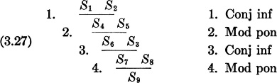
In the tree (3.27) every horizontal bar indicates an inference whose designation is given in the right-hand column. Every statement occurring under a horizontal bar is inferred from the statements immediately above that bar. Statements that do not have a horizontal bar directly over them are of types D1, D2, D4. The form of the tree (3.27) can be indicated by a simple line sketch, as in Fig. 9. In the sketch of Fig. 9, the nine short line segments represent the nine statements of the tree (3.27). Each of the four branch points represents an inference, and the segments leading downward from the branch points represent the statements “S4, S6, S7, S9”, which are all of type D3. The remaining segments, or branches, represent the statements “S1, S2, S5, S3, S8”, which are of types D1, D2, D4. Of course, the bottom segment, or trunk, represents “S9”, the statement to be proved.
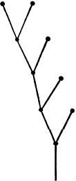
FIG. 9. A line sketch consisting of nine short line segments and four branch points.
The tree form of a demonstration is not as compact as the sequence form, and may appear as quite an impressive structure if the theorem it demonstrates is at all complex. However, the tree form brings out clearly the role of inference in a demonstration, and is perhaps for this reason easier to understand than the sequence form.
Recall that the statement (3.21)

asserts the existence of a demonstration as defined in Sec. 3.8. To prove that (3.28) is true, it is enough to exhibit a suitable demonstration. We shall also consider as proof that “P” follows from “A1, …, An”, any sound argument that shows the existence of a demonstration of (3.28), even though the demonstration is not actually exhibited. Such proofs arise when demonstrations are abbreviated by the use of previously proved statements.
In the definition of Sec. 3.8, no provision is made for using a previously proved statement as a step in the demonstration. This provision was avoided for the sake of a simple definition. But, if only demonstrations are allowed as proofs in plane geometry, for instance, then one is forced all the way back to the axioms in every proof. This would not be such a hardship in the case of the earlier theorems, but would require inordinately long proofs for the later theorems of geometry.
Assume that

had already been demonstrated, and it is desired to prove

Suppose now that there exists a sequence of statements,

where “Sk” is the same as “P”, and each “Si” is one of “A1, A2, …, An”, or is in the form of a valid statement formula, or follows from earlier statements in the sequence by means of an established inference rule, or is the same as some earlier statement in the sequence or is the statement “B”. If “B” occurs one or more times in the sequence (3.31), then (3.31) need not be a demonstration of (3.30), but it is clearly a demonstration of

since then the occurrence of “B” in the sequence comes under the condition of being one of the statements “B, A1, A2, …, An”. From (3.29) and (3.32) it follows that there exists a demonstration of

To see this, in (3.25) replace, “B1” by “B”, “B2” by “A1”, “B3” by “A2” …, “Bm” by “An”.
It is easy to see that any demonstration of (3.33) is also a demonstration of (3.30). Thus, while the sequence (3.31) is not a demonstration of (3.30), it is a proof of (3.30) because it ensures that a demonstration of (3.30) exists.
We illustrate with a proof of a theorem of natural numbers, which depends on (3.26), proved in Sec. 3.8. Suppose we take as axioms for natural numbers, the closure, associative, and commutative axioms for addition, and the transitive axiom for equality:
Let us prove

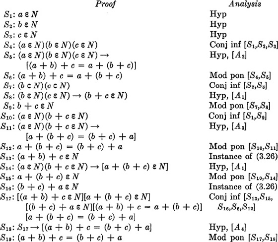
In spite of its length, the proof is not a demonstration because “S13” and “S16” do not satisfy any of the conditions D1 (hypothesis), D2 (form of a valid statement formula), D3 (deduction from an established inference rule), or D4 (a repetition of an earlier statement in the sequence) of the definition of a demonstration. But, if the first eight steps of the demonstration of (3.26) are inserted in the proof after “S12”, and the same steps (with an obvious change of notation) are inserted after “S15”, the resulting sequence of statements will be a demonstration. The demonstration will have sixteen more steps, and many repetitions.
While not a demonstration, the proof has a tree form:
We have circled “S13” and “S16” since if the tree were a true demonstration, these statements would not be simple branches, but would have more branches above them, namely, tree forms of the demonstration of (3.26). The tree may be sketched as in Fig. 10.
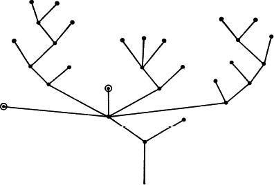
FIG. 10.
The sketch (Fig. 10) shows seventeen branches, two of which can be thought of as trunks of the system of branches in Fig. 9.
As a first abbreviation of the proof of (3.34), an obvious step is to omit the conclusions of conjunctive inferences. This type of abbreviation would eliminate “S4, S7, S10, S17”. To leave out “S4” where it first occurs in the proof is, in effect, to merge it with the modus ponens inference yielding “S6”. With these mergers modifying the tree it may be sketched in as in Fig. 11.
If now it is agreed to abbreviate by omitting the major premises of all modus ponens inferences, then “S5, S8, S11, S14, S18” will be eliminated. So much abbreviation might make the proof hard to follow, and so a clue to the tacit major premise will often be provided in the analysis column opposite the conclusion of the inference in question. With these abbreviations, the tree is further modified and its sketch appears in Fig. 12.
FIG. 11. Line sketch of Fig. 10, modified by eliminating certain line segments.
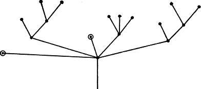
FIG. 12. Line sketch of Fig. 11 further modified by elimination of certain line segments.
The sequence form of the proof is reduced by these abbreviations to the following ten statements:
Another common type of abbreviation is the combination into one statement of several statements of the same kind. In the latest version of our abbreviated proof, we might choose to combine “S1, S2, S3” and “S9, S15” and “S13, S16”, respectively, into three statements, thus obtaining a proof having just the following six steps.
This final form is about what would normally be offered as a careful proof of (3.34), although the analysis would not usually contain any reference to modus ponens.
It is well to observe in the preceding sample demonstrations exactly what was demonstrated. In (3.26), the existence of a demonstration shows that “(a + b) + c ε N” can be correctly deduced from the four statements

The demonstration did not demonstrate

Similarly, in dealing with (3.34),

we did not show that

However, in both cases, it is (3.35) or (3.36) that we would really like to demonstrate. In general, we need to modify the foregoing notions of a demonstration in order to prove theorems. A theorem of geometry, for instance, is regarded as a statement that can be deduced from the axioms of geometry. Theorems of geometry are usually in the form of conditionals. Suppose “P → Q” is the translation for a geometry theorem, and “A1, …, An” are translations for axioms. Then the usual problem is to prove that “P → Q” can be deduced correctly from the axioms. What is wanted is a demonstration of

A typical procedure is to deduce “Q” from the axioms and “P”, that is, to demonstrate

Once (3.38) has been demonstrated, it is customary without further ado to assert that the theorem has been proved. The tacit proposition is “If (3.38), then (3.37)”. The principle involved may be stated in general form as follows:

While we shall take (3.39) as a logical principle with no attempt at proof, it should be noted that (3.39) is in fact a theorem of logic, and proofs of it can be found in current textbooks on mathematical logic.1 The form (3.39) asserts that if there is a demonstration S1, S2, …, Sr of A1, …, An, P Q, then there exists also a demonstration  . The usual proof consists in showing how to construct the S*′s given the S’s.
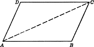
FIG. 13. Parallelogram ABCD.
As an example of application of the deduction principle consider the plane geometry theorem:
If a figure is a quadrilateral, then, whenever its
(3.40)
opposite sides are equal, it is a parallelogram.
Using the notation of Fig. 13, let “P”, “Q”, “R” be translations as follows:
P: ABCD is a quadrilateral.
Q: AD = BC and AB = DC.
R: ABCD is a parallelogram.
Then we take the following instance of (3.40) as the theorem to be proved:
(3.41) P → (Q → R).
The usual proof begins with the assumption of “P” and “Q”, and goes on to show that the diagonal AC divides the quadrilateral into two congruent triangles, and from this result deduces that the opposite sides are parallel, and hence “R”. Such a proof establishes

but it is (3.41) that we desire to deduce from the axioms. It is at this stage that the deduction principle may be used to obtain

Note that we have not actually produced a demonstration of (3.43), but assert on the basis of existence of a demonstration of (3.42) and the deduction principle that a demonstration of (3.43) exists. However, (3.43) is still not what we want. We have to use the deduction principle once more to obtain

Use of the deduction principle is tacit in virtually all proofs in plane geometry. Surely a high school student who succeeded in demonstrating (3.42) would be happy to write Q.E.D. and would not be conscious of the need to say anything more. A plane geometry student bent on proving a theorem in the form “H → C” almost surely looks upon the conclusion “C” as the thing he is trying to prove true. While a mathematician is quite clear that it is “H → C” that he is trying to prove, he normally uses the same procedure as the high school student, namely, he assumes “H” and gives a demonstration for

and for him also the deduction principle is tacit in the proof of

It is only when one tries to give precision to the notion of a proof that the distinction between (3.45) and (3.46) becomes urgent. In many cases in mathematics, care must be exercised in the use of the deduction principle, and we shall have to reconsider it in a later section when we deal explicitly with proofs of quantified statements.
1 J. Barkley Rosser, Logic for Mathematicians, p. 75, New York: McGraw-Hill Book Company, Inc., 1953. Alonzo Church, Introduction to Mathematical Logic, Part I, p. 10, Princeton, N.J.: Princeton University Press, 1944. Stephen Cole Kleene, Introduction to Metamathematics, p. 90, Princeton, N.J.: D. Van Nostrand Company, Inc., 1952.
The conventional proof of a theorem of geometry has the following pattern:
1. The theorem is stated.
2. A figure is drawn and lettered.
3. The theorem is restated in terms of the notation of the figure, as “P → Q” or often in the form: Given: “P”; To Prove: “Q”.
4. An abbreviated demonstration is given of “Axioms, P Q”.
5. By a tacit use of the deduction principle it is considered that “Axioms P → Q” has been proved.
6. Although “P” and “Q” are statements about the particular lines and points of Step 3, it is assumed that Steps 2 to 5 are proof of the theorem, which is a statement about all such lines and points.
Let us investigate conventional proofs with respect to Steps 2 to 4. Among the abbreviations occurring in Step 4 are found the types mentioned in Sec. 3.10, namely,
a. Use of proved theorems
b. Omission of conclusions of conjunctive inference
c. Omission of the major premise in modus ponens inference
d. Combination of steps of the same type
However, additional abbreviations are commonly employed, and certain conventional words and phrases occur in the analysis column.
As we have seen (Sec. 3.8), a demonstration consists of a sequence of statements satisfying certain formal requirements. The analysis of a demonstration is not essential to it, and consists of comments about the form of the statements in the demonstration. In contrast, the analysis column of the usual abbreviated proof in geometry contains statements essential to the proof and is not just a sequence of comments on the form of the statements in the “statement” column. If then, such a proof is not to be hopelessly abbreviated, it must be accompanied by an analysis, or a column of “reasons”. However, the analysis also serves a pedagogical purpose in that it helps a teacher to determine to what extent a student knows what he is doing. Furthermore, writing out definitions and theorems and axioms for the analysis helps a student learn these theorems and definitions and axioms. For these reasons, it is commonly the “reason” column that is emphasized in teaching students how to write out proofs. They are often given explicit instructions about the statement to which the “reason” corresponds. With the admonition “Every statement must have a reason” ringing in his ears, a student thinks of the “reason” as something that assures the truth of the corresponding statement. This is not at all the role of the analysis column of a demonstration as described in Sec. 3.8.
It is not really very hard to write out proofs that, even though abbreviated, are more in the spirit of demonstrations. It is only necessary to transfer some statements traditionally appearing in the reason column to the statement column. Let us examine a typical conventional proof and see how this can be done. We shall follow the pattern for a conventional proof in geometry given on page 91.
Theorem: In a parallelogram, the diagonals bisect each other.
Draw a figure (Fig. 14) and letter it. State the theorem in terms of the notation of the figure and in the “Hypothesis-Conclusion” form:
Hypothesis: ABCD is a parallelogram with the diagonals AC and BD meeting at M1 (Fig. 14).
Conclusion: AM = MC and BM = MD.
We are now ready to embark on Step 4 of the pattern of proof, page 91.
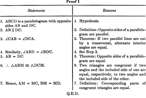
Note the further abbreviation that leaves tacit the proof that ABM and DCM are triangles.
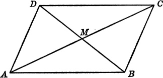
FIG 14. Parallelogram ABCD with diagonals AC and BD intersecting in M.
Now let us rewrite the proof by shifting the statements and definitions over into the statement column. This involves no more writing than before, except that the use of modus ponens is indicated.
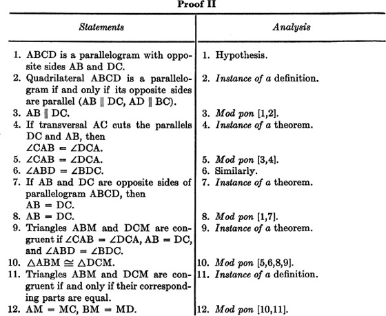
In comparing these proofs, notice that the extra words of Proof II are in italics. It is worth observing that there are few words in Proof II not appearing in Proof I, but Proof I makes no reference to modus ponens. If in Proof II, modus ponens is to be tacit, then each of Steps 3,5,8,10, and 12 would be merged with its preceding step, thus yielding a seven-step proof as in Proof I. For instance, Steps 3 and 2 might be merged as follows:
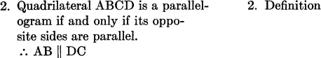
If such mergers are to be considered proper, it may be helpful to make an agreement that  always introduces the conclusion of a modus ponens.
Proof II as it stands, without these mergers, is not really any longer than Proof I. In particular, every statement in the statement column of Proof II occurs somewhere in Proof I. In Proof II, the analysis is truly descriptive and not at all necessary to the proof. Also, the analysis is not as necessary pedagogically as is the set of reasons in Proof I. If a student wrote out the set of statements 1 to 12 of Proof II without any accompanying analysis, would you not be inclined to believe that he knew what he was doing?
In the analysis of Proof II, consider Step 7: there we say “instance of a theorem” rather than just “theorem”, because the theorem in question is
The opposite sides of a parallelogram are equal,
which is a general statement about all parallelograms, whereas the statement in Step 7 is a statement about ABCD which, though unknown, is a fixed particular parallelogram. Of course, the statement in Step 7 is true, because the theorem is true for all parallelograms.
Proof II is not only easier to follow than Proof I, but is much easier to describe. Every statement in the statement column is either the conclusion of a modus ponens from earlier statements, or a statement considered true because it is part of the hypothesis, or an instance of a theorem, an axiom, or a definition. The analysis simply notes that the statements have these properties. As an aid in following the proof, the analysis of a modus ponens conclusion indicates the major and minor premises by numbers. No such simple description is possible for Proof I.
As the geometry course progresses and it is felt that abbreviations are desirable, Proof II can be abbreviated as easily as Proof I. If, for instance, it is desired to use “A.S.A.” to indicate the congruence theorem in Proof I, Step 6, it can as well be used in Proof II, Step 9.
1 Of course; we are not really dealing with an instance of the theorem in question, because the “intersection of the diagonals” is part of the conclusion. However, it is a rare geometry book that supplies the necessary axioms to prove this, so we shall not attempt it here. In fact, we are proving “if the diagonals of a parallelogram intersect, then they bisect each other”.
Now, let us consider the relationship between a theorem and its corresponding figure. In a sense, we can regard the streaks and dots of chalk we draw on a blackboard as real interpretations or models of the abstract lines and points of geometry. This is probably our attitude when carrying out straightedge and compass constructions. However, when we draw a figure in connection with a geometric proof, it is probably safer to regard it as a symbol, or a collection of symbols, naming the lines and points with which the theorem is concerned. In proving the theorem on page 92, it is necessary to talk about the parallelogram and its diagonals. In order to talk about the parallelogram, we need a name for it, such as “the parallelogram”. In fact, we used “ABCD” as a name for the parallelogram. This is a fairly good name, because we also used “A”, “B”, “C”, and “D” as names for the vertices of the parallelogram, and this relationship between the names of the vertices and of the parallelogram helps us to think about them more clearly. Figure 14, including the letters, contains a name for the parallelogram, as well as names for vertices, diagonals, sides, and so on. Let us imagine that the streaks of ink naming diagonals are removed from the figure, along with the letter “M”, then, what is left is a symbol or name for the parallelogram. Since this figure and “ABCD” are both names of the same parallelogram, they could be used interchangeably in any statement about the parallelogram. The figure is, perhaps, a better name for the parallelogram than is “ABCD” because it carries more information for us. From the figure we would expect to name one side of the parallelogram “AB”, for instance, while we would not have that expectation just from the name “ABCD”.
It is not normally very convenient to use pictorial names in written statements. One does not write
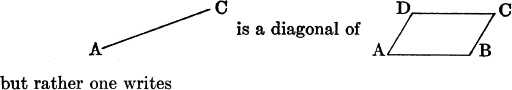
AC is a diagonal of ABCD.
The figure is not used in statements, but is nevertheless useful because it can be thought of as a collection of names carrying more accessible information than the literal names used in statements. For example, in the statement
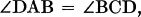
the angles are named by the literal symbols “∠DAB” and “∠BCD”. It is surely helpful to look at the corresponding names for these angles to be found in the figure. The figure suggests relations between these angles and other parts of the parallelogram. In addition, the figure aids in comprehending the statement of equality of angles in relation to other statements that might be made about the parallelogram.
This use of a figure is a two-edged affair. Relations existing between the parts of the figure do not necessarily correspond to relations between the parts of the parallelogram. Anything suggested about the parallelogram by its figure must be verified. But the pictorial names, or figures, used in geometry are very clever names and their suggestions are often so powerful that one sometimes accepts them without proof. In the proof of the theorem, page 92, the figure suggests so strongly that AC and DB intersect, that not one student in a thousand feels any need for proving it. Literal symbols are not so seductive. One is not, for instance, inclined to assert that the diagonal AC contains two letters just because its name “AC” contains two letters. It is perhaps for these reasons that both literal and pictorial names are used. The pictorial symbols are useful because they are highly suggestive but are for this reason dangerous. To verify the suggested relations, one writes out proofs using literal symbols to avoid the danger.
A geometry teacher has a delicate job here. On the one hand, he has to train a student to make the utmost use of figures, but on the other hand he has to be sure that the student does not identify the figure with the geometric abstraction of which it is a name. The conventional language of geometry tends to encourage identification of a pictorial name with the thing it names. For instance, the same word “line” may be used to name the undefined geometric element and the chalk streak or ink deposit of a figure. The direction
Draw the line AC
may suggest to the student that he is supposed to create a line joining A and C, which points presumably are not at the moment joined by any line. This is, of course, absurd. One can, however, draw a picture of the line AC.
It is common practice in some textbooks to state as an axiom:
One and only one straight line can
be drawn through any two points.
This is not at all intended to be a statement about figures or pictures, but is supposed to be an assumption about the abstractions line and point. The language is misleading, but common. It would be far better to state the axiom:
There exists one and only one straight line
through any two points.
The language of construction problems is especially loaded with expressions that incline one to think about the figure rather than the abstraction for which the figure stands. In particular, it is common practice to have geometry students describe a construction just after stating a theorem in the Given-To Prove form and before embarking on the proof. Then, in the proof, “construction” may be offered as a reason for a step. If the construction is really a description of the figure, then “construction” can never be offered as a reason for a statement in the proof of the theorem, for such a statement is never an assertion about the figure. Statements used in the proof of the theorem must be statements concerning the abstract configuration of points and lines, like triangle or parallelogram, mentioned in the theorem and not statements about the figure. The use of the word “construction” might be justified if the existence of the lines and points constructed is proved, but such proof belongs with the rest of the proof and seems out of place if given as a preliminary. Consider a conventional proof of a theorem involving an isosceles triangle, where it is understood that all the usual congruence theorems about triangles have been assumed as axioms.
Theorem: The base angles of an isosceles triangle are equal.
First we draw a figure (Fig. 15) and letter it.
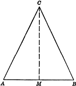
FIG. 15.
Then we proceed as follows:
Hypothesis: ΔABC is isosceles with AC = BC (Fig. 15).
Conclusion: ∠CAB = ∠CBA.
Construction: Draw CM joining vertex C with the mid-point M of AB.
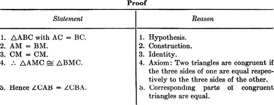
The proof is incomplete because the construction has not been proved.1 If the construction is to be justified, its proof might as well occur in the main body of the proof, perhaps as follows:
Hypothesis: ΔABC is isosceles with AC = BC (Fig. 15).
Conclusion: ∠CAB = ∠CBA.
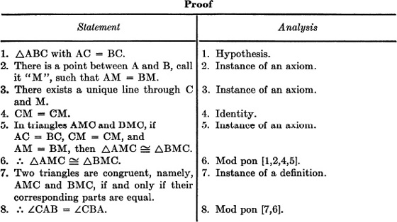
The use of the word “identity” in both proofs is worth a comment. In order to be of use in proving the congruence of triangles AMC and BMC, one must interpret “CM = CM” as asserting “The length of the side CM of triangle AMC is equal to the length of side CM of triangle BMC”. Of course, these sides are the same line segment CM, and the equality is an instance of an axiom. All of this is abbreviated in the statement “CM = CM” and the reason “identity”.
EXERCISES
Look up proofs of the following statements or make your own proofs. Try to write each proof in the spirit of Proof II, Sec. 3.12, with an analysis column that is “pure” analysis.
1. Prove: The sum of an even number and an odd number is odd.
2. Prove: A diagonal of a parallelogram divides it into two congruent triangles.
3. Prove: The sum of two even numbers is even.
4. Prove: sin2  + cos2 = 1.
5. Prove the law of sines.
6. Prove: If n2 is even and n is an integer, then n is even.
7. Prove: In a circle, an angle formed by a tangent and a chord drawn to the point of contact is measured by one-half of the intercepted arc.
8. Prove: (ab = 0) → (a = 0)∨(b = 0), where a and b are real numbers.
9. Prove: A point is on the bisector of an angle if and only if it is equidistant from the sides of the angle.
10. Prove: The bisectors of the interior angles of a triangle are concurrent.
1 We might also note that, though quite obvious, it was not established that AMC and BMC are triangles. To show them triangles, we might argue: A, M, and B are collinear by definition. If A, M, and C are collinear, then A, B, and C are collinear since there is a unique line through A and M. But A, B, and C are not collinear by the definition of a triangle. Therefore A, M, and C are not collinear by contrapositive inference, and AMC is a triangle by definition.