CHAPTER 3
Real Time Analysis

Noise Generators

White noise, (the sound heard when a radio or television is tuned between channels) consists of all audible frequencies at equal level. Pink noise is similar but has been put through a filter that rolls of 3 dB per octave. Here the higher the frequency, the greater the attenuation. This is done because pink noise is used with -octave analyzers whose bandwidths become wider as the frequency increases. For example, between the first two center frequencies, 16 and 20 Hz, there are but 4 cycles. On the top end, between 12.5 and 16 kHz, there are 3,500 cycles! In other words the level of power of the bottom bandwidths of -octave spectrum analyzers is much lower than it is at the higher frequency bandwidths. By using a filter that progressively attenuates more level as the frequency increases, we end up with a display that appears flat on -octave analyzers. Everything becomes all matched up perfectly, when set at ISO center frequencies and ANSI bandwidths.

As an aside, the names white and pink relate to the light spectrum, wherein red equates to lower frequencies and a mixture of the whole spectrum produces white light. Due to its high-frequency roll-off (and resulting low-frequency emphasis), it adds a little red to the white and is therefore “pink” in color. (Crazy world, right?) Like white noise, pink noise is a sequence of all frequencies generated randomly or at least pseudo-randomly. It is because of this randomness that we are required to average multiple readings to achieve accurate results. The Alan Parsons and Stephen Court Sound Check CD has individual -octave bands at ISO center frequencies. These are more stable than a pink noise generator. In addition the “one band at a time” approach to system adjustment is easier on the eyes, ears, and equipment, as both white and pink noise are not enjoyable listening, especially when levels must be high to overcome background noise.

Using -octave analyzers has become very simple because of the addition of microprocessors, but care must still be taken so as not to over-EQ. The operator must proceed in a slow, orderly, and thorough manner. If any cutoff filtering (low or high pass) is being used, it must be introduced before the processing because it can have an effect on the other settings. After making any adjustment to a -octave EQ, the system should be given a bit of time to “settle in” or stabilize before proceeding to the next band to be adjusted. After the EQ adjustment has been completed, it is critical that the system be given a good “listening to,” using very familiar programming to make sure the end result is acceptable to all intended users.

Real-time analyzers (RTAs) are capable of obtaining a reading of the whole spectrum in one shot. They are able to follow changing signals and also to provide a graphic readout. This is way faster than sequential and even swept analysis. This is all possible because RTAs have a set of filters that match ISO center frequency and ANSI bandwidth standards. In short, a signal is injected into the system, amplified, picked up by a calibrated microphone, and then put through a bank of filters that divide the signal up into multiple frequency bands. These are then scanned, and their levels detected, averaged, and presented on some form of display for ease of viewing and adjustment. This is done very quickly, just as it happens in real time, hence the name.

The speed at which these results are generated made it necessary to have a display that was capable of constant updating while providing ease of viewing. In the early days, this screen was a cathode ray tube much like the ones used in old television sets. These were bulky, delicate, and expensive, but compared to sequential analysis, they were a joy to use and these early RTAs gave very accurate readings of the audio spectrum. By the 1980s, with the use of smaller and less expensive components, such as integrated circuits and less bulky and cheaper LED matrixes, the cost of RTAs dropped radically, even though many of these included microprocessor control and memory functions!

Today RTAs have many different features and capabilities. Most folks consider these as use-once devices unless acoustical parameters in the environment have been changed. Therefore, many studios use one just for a day or two to take measurements and make adjustments. However, as a continuing display tool, a spectrum analyzer can be remarkably helpful. This may be obvious when performing maintenance and calibration routines, but I loved to have one all wired in while I was recording and mixing too. Look, I can walk over to a 31-band graphic EQ during a live show and pull down the exact fader required to reduce even a slight amount of ring. My ears have been trained for over forty years to discern frequencies, but in the studio, when my attention may be focused on one particular instrument, some other sound, or worse yet, a lack of sound may slip by unnoticed.

After having done a good deal of recording with a Klark Teknik DN60 RTA sitting right up on the console’s meter bridge, I can understand why some manufacturers outfit their consoles with spectrum analysis capabilities. I can honestly say that its use not only improved the overall sound, but also increased my ability to perceive spaces in the content. I also found that while clients were at first amused by the “light show” movement of the display, they soon started adjusting the frequency content of their instruments’ sound and toned down the excessive use of effects devices. The DN60 featured memories, peak hold, a built-in switchable “A” weighting network, microprocessor control, variable response time, and much more. It provided its own signal output in the form of a quality pink noise generator. Output was via an XLR panel connector, and its level was continuously variable (via a rear panel pot) from −6 dBm to +2 dBm.

Gold Line makes a complete range of test equipment for sound contractors including: real-time analyzers, SPL (sound power level) meters, frequency counters, sine-wave generators, gated pink-noise generators with timed pulses, decibel meters, impedance meters, a distortion analyzer, and systems that have 30 memories, a printer port as well as RS232 interface. This test system made up of individual components allows you to go with only what you need, but its extensive range also includes a RT 60 reverb timer, loudspeaker phasing, as well as frequency-response measurement tools. They even give you the option of measurement microphones at two price levels. It can take a lot of test gear to get and keep a monitoring system honest.

I’ll never forget the first time I used a Gold Line portable 31-band, third-octave, real-time analyzer. You draw an outline of the walls, ceiling and floor; pump pink noise through the monitors; and walk around the room pointing the microphone into suspected areas and mark down all problem positions with frequency notations on the drawings. I was then able to say to the studio owner: “You have a 4 kHz-flutter problem between these two surfaces, a low-frequency peak at these locations, and a phase dropout at the listening position due to reflections from these locations on those two surfaces.”

Later with the Neutrik strip chart recorder, I could hand them hard copy. Then with the Klark Teknik, averages of multiple reverberation decay curves were added! A newer DN600 model RTA from Klark Teknik offered both ¹/₆- and stereo or dual -octave analysis plus displayed sum and difference and had built-in A and C scale filtering. The display could be set for peak or average, and it had a peak hold function. Its internal signal generator produced sine and pink noise signals, and had tone burst (for reverb timing) and sweep capabilities. The DN600 handled reverb timing without the need of an optional add-on. It could store 32 memories and also had a printer port for direct printer output, but to me, the most amazing addition was this unit’s ability to directly interface with the DN3600 programmable dual-channel -octave equalizer. Hold onto your hats, because the combination of these two devices equated to: automatic correction of equalization settings!

But everyone should shoot a room the old-fashioned sequential way at least once! The insight gained as far as the benefits of microprocessor control, real-time averaging, and synchronized sweeps will clue you in on why we were happy to spend thousands on test equipment that had these capabilities back in the 1980s. The fact is, that today, some inexpensive software along with the price of a sound card and a microphone can turn your laptop into a real-time analyzer, which can put you in the game. However, attention to detail still separates mere amateurish attempts from the kind of precision measurement that provides conclusive and reliable results.

Measuring Reverberation Time

Measuring reverb is pretty much the same as measuring frequency response, but now your speaker output levels for each frequency tested not only have to be equal, they also have to fit into a fairly narrow dynamic range because too low an output may not trigger the measurement and too high can cause false triggering. These days this is not usually a major problem because most reverberation timers automatically turn the noise source on and off and provide the correct timing synchronization.

Reverberation timers are usually composed of a signal generator that outputs a pulse, spark, pink-noise burst or continuous sign wave (which, once it has built up in the room, is then cut off), timing circuitry, and a synchronizer that locks the two together. A microphone input and preamp completes the package. Here you are checking to see if the decay is unusually long or short at a particular frequency. Some instruments also provide reverberation decay curves across the complete audio bandwidth.

A controllable electronic noise source is used as a signal for these measurements. This signal is fed into a power amplifier and loudspeaker to bring it up to a level above the room’s noise floor. Impulse noise as from a starters’ pistol or a punctured balloon can be used as the test signal, but the noise they produce does not contain equal energy at all frequencies. Furthermore, the impulses generated by these sources can be variable to the point where they may not trigger the test instrument to capture the data reliably, which is obviously essential to accurate measurement. Because reverberation time varies with frequency, these measurements are usually taken in one-third or at least octave bands. These tests are performed in real time simply because a large number of measurements must be taken at a number of different locations in the room to provide an average result that is representative of the whole room. At least a half dozen measurement positions are required, and this can end up meaning dozens upon dozens of tests. Some real-time analyzers not only turn the noise source on and off to provide the correct timing, but their internal microprocessors also gather, analyze, and store the data. Hey, studio time = $ money, so interruptions to the work schedule must be kept to a minimum.

The Klark Teknik Optional RT-60 Reverberation Timer

The pink-noise source in the DN60 RTA was driven by a line amp that was gatable. The gating was controlled by a microprocessor, and it enabled very accurate timing of the output on and off switching. Reverberation decay time is determined by first removing a signal and then measuring the time it takes for that signal to drop 60 dB. To do this accurately, the sound source level might have to be set very high level (depending on the level of background noise). To ease this measurement process, here the decay time is calculated from a smaller decibel drop. Through an internal “communications” card, the RT-60 optional reverb timer could control the DN60’s microprocessor.

Once the RT-60 was hooked up, it was included in the DN60’s self test, and this dual unit was capable of measuring reverberation time. It sampled the decay every 550 microseconds, averaged 16 of these samples, and stored them until the cycle was finished, at which point it had 790 8-millisecond samples. The DN60/RT-60 could measure a decay from 0 dB down to −30 dB, or any range in between, with as little as a 2-dB drop and calculate (extrapolate) a measurement for a 60-dB drop. The parameters of the decay curve could be changed after the measurement without affecting the original measured value.

It is normally necessary to take many tests with any reverb timer and average these together for more precise readings. This dual unit did your averaging (accumulating) for you up to 32 readings and could measure and accumulate either the full bandwidth or any individual band. Since the RT-60 controlled the microprocessor, some of the functional parameters of the DN60’s switches were changed. Here the peak/hold switch now showed at which frequency band the measurements were taken. The peak/average switch controlled the pink-noise turn-on. This was important to saving your ears, as it allowed you to start the noise just before taking a measurement. The RT-60 was also very user-friendly in that it told the operator via the readout when the unit was properly set up for measurement. It indicated running and calculating, as well as accumulating modes, and more. Once measurement was completed it showed a graph of the decay curve. Here the -octave frequency bands were converted into time columns. The display’s time parameters could be changed after the measurement to one of three settings: 16, 64 or 208 milliseconds per column. This decay curve could also be stored in the DN60’s memory. When recalled, it would show if accumulation was used, how many accumulations were made and the frequency band measured; yet the window and time parameters could still be changed. Furthermore the RT-60 accumulator could be used in the spectrum analysis mode to average up to 32 frequency response measurements. All this gave the operator a very powerful tool to work with. I was able to check studios, control rooms, as well as time digital reverbs, tape reverbs, and chambers, all with ease.

However if all we need is a clue to give us insight into possible room anomalies, simple reverberation time only tests can often do the trick. A good example of how easy reverb measurement can be is provided by using Gold Line’s GL60 reverberation meter. Here the microphone, timer, and display are built into one small 5″ × 5″ × 2¼″ box, and because it runs on two 9-volt batteries, it is completely portable. This unit mates with Gold Lines’ PN3A pink-noise generator which is only 2¼″ × 4″ × 1½″ and runs on a single 9-volt battery. In “continuous” operating mode its output is 95–97 dB (ref 110 dB SPL). In RT60 mode it puts out 11-second bursts with the time off in between each burst being variable from 10 to 150 seconds. These two units will run you only about $600.00.

Okay, say you have excessive levels at 125 Hz. Now with close micing, we can see if the reverb time at 125 Hz differs in various parts of the room. In other words, where are the best places to add acoustic corrections? The GL60 takes measurements at six different frequencies: 125, 250, 500, 1000, 2000, and 4000 Hz. Sound familiar? That’s right, the same frequencies at which absorption coefficients are rated. This ends up being pretty handy in that, should you have a problem at 250 Hz (or at any of those frequencies for that matter), you simply look for a material or acoustic panel that has a narrow band peak in absorption at that frequency.

Acoustilog IMPulser

Folks used to input pulses into their system, mic the room, and monitor the output on an oscilloscope. They would vary the frequency or timing of the pulse train until the resonant frequency caused a flutter echo. When they measured the distance between the flutter peaks, they had the timing. Multiplying that by the speed of sound and dividing the result in half gave them the distance. Sounds a bit complicated? Well, it could be quite cumbersome with all the wiring, microphone phantom power supply, preamp, amp, speaker, and scope, but a company called Acoustilog, which was run by an acoustician named Al Fierstein, used to make a small portable box called an IMPulser. Most people purchased it because it rendered absolute confirmation of correct: system, speaker, individual driver, and even microphone phasing, but outside of a mic and a scope, it covered everything needed for these tests all by itself! It generated a positive pulse, which had variable width (40 Hz to 10 kHz), rate (0.3 to 10 pulses per second), and level. You simply injected the pulsed signal into the system, and used a mic to pick up the speaker/room output. The IMPulser not only provided the phantom power to the mic but also amplified its signal. This was then sent to the scopes’ trigger input, and the direct pulse output was connected to the vertical input. The result was an irrefutable display, showing you either a positive in-phase (above center line) or negative out-of-phase (below center line) pulse. But when used to test the acoustics of a room, you could actually see flutter echoes, slap-back delay pulses and ringing waveforms (Fig. 3.1).

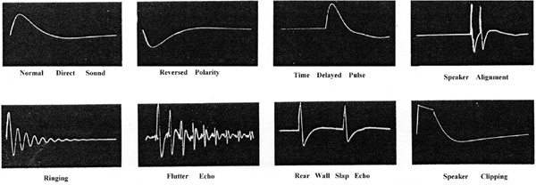
FIGURE 3.1 Examples of Acoustilog IMPulser oscilloscope signal traces.

Using the scopes’ screen graticules (divisions) and varying the time base, you could get a pretty good idea of the timing and then do the math, but Acoustilog also made a fairly inexpensive reverberation timer that saved you the trouble. Finding the boundary that is causing a flutter, slapback delay, or phase cancellation is a lot easier when you know its distance from the microphone. The whole idea is to know exactly what you are dealing with before you start to make adjustments to your room or purchase acoustic materials or premade panels. Getting everything right from the start is crucial to keeping cost-inflating mistakes to a minimum. This is why I like using both reverberation time and frequency response measurements and also why we go through all the trouble of working out the mathematics to get an idea of the expected reverb time by using the average absorption coefficient of all of the room surfaces, which is well covered in Part II. So now you will have a very good idea of how to perform all three checks.

Equipment Rental

Unfortunately I cannot tell you where to rent real-time analyzers and reverberation timers on the cheap because these devices have to be calibrated every time they are sent out. I put a good deal of time into researching this possibility, and except for the following two came up blank. If you reside in England, you can “hire” a top of the line Nortronics NOR 118 handheld RTA/reverberation meter for 32 pounds ($51.38) per day, minimum of four days plus shipping and, what I am sure are, some hefty insurance fees for this multi-thousand dollar device. States-Side, Acoustical Surfaces, who sell the Phonic PAA3 RTA/reverb timer for about $500 will also rent one to you with the USB interface for $250. The interface is important here because it is much easier to view 31 bands of information on a computer monitor instead of the small LCD screen. Bottom line? I might not recommend these to the small studio owner simply because the cost, while fair, equals the price of a premade acoustic panel which might out and out solve the problem. But do go online and check out what is arguably the “state of the art” Nortronics NOR 118 just so that you have some “dream” device to compare to prospective measurement equipment at noisemeters.com. The Phonic PAA3 is all inclusive and you can check out the full range of its capabilities at http://www.acousticalsurfaces.com/soundlevel_meter/phonic_paa3.htm?d=30.

Acoustic Measurement with a Laptop

Now let’s look at a very simple, and thus, commonly used room acoustics measurement setup that’s a combination of a microphone, preamp, sound card, laptop, and software. Let’s start at the software end. How about using freeware?

First download a free version of TrueRTA™ software. I have used this, and it is a very good spectrum analysis tool. The free version provides a pretty comprehensive generator, analyzer, and display combination. The generator can output sine, triangle and sawtooth waves. You select the frequency (5 Hz to 24 kHz) and level (minus 150 dBu to plus 20 dBu). The generator also outputs impulse and pink noise (up-graded versions, which you have to pay for, add white noise and sweep modes). On the analyzer side, the free version provides only an octave or 11-band readout, but you can still select the top-level reading to be anything between positive 10 dBu to negative 90 dBu. And the bottom of the scale can be set to anything between positive 10 dBu and minus 160 dBu. The high frequency limit of the display can be set from 50 Hz to 50 kHz and the low from 10 Hz to 10 kHz. Finally the speed can range from slow 20 Hz (as in twenty times per second), medium 40 Hz, or fast 80 Hz. Straight out I do not expect you to understand all of the above technical information, but hey, it’s a free download so jump on the chance to check it all out. I guarantee you that in a fairly short amount of time you will have it all down.

Next is the computer. Most everyone today has a laptop with at least a headphone jack output and a microphone jack input (usually inch). The generator output appears from the headphone jack, and the analyzer input is on the microphone jack.

Here we run into our first problem: the headphone output is stereo and the microphone input is mono. You could simply patch a stereo jack-to-jack cable from the headphone out to the microphone input. However, this would short circuit one side of the stereo output, and I am flat out against shorting anything out in audio. There are ″ stereo to mono adaptors, but they combine the left and right sides into the mono jack. The real deal here is to cut the end off of a ″ stereo to ″ stereo cable (leave enough cable attached to the “cutoff” end so that you can use that side of the cable for another adaptor). Now solder a ″ mono jack to the cable, omitting the “ring” conductor. You can then plug the stereo plug into the headphone and the mono plug directly into the microphone jack, and work the input and output variables of this software to the bone until you have it all figured out.

Then you get to take the signal generator output from the headphone jack, add an adaptor if needed to the ″ mono plug and feed the signal into anything you want. An equalizer is a great place to start. Feed the output of the EQ into the analyzer (microphone) input, and you will be able to see exactly what that EQ is doing in terms of an octave or 11-band spectrum. Right quick you’ll pick up on the need for more bands, but you’ll have gained a huge insight into spectrum analysis, and also understand the need for more professional analogue-to-digital conversion that can be had from a dedicated sound card.

But in order to perform room analysis, you are going to need a microphone, a preamp, and a power supply. So go online and check out a bunch of acoustic test microphones just so you are aware of the differences. Most important here are a flat as possible frequency response, low noise, and the most sensitivity you can afford. Flat frequency response and low noise are straight ahead, but sensitivity should be explained.

Although you are simply measuring levels above and below a reference level, you are always dealing with background noise especially when it comes to reverb time so let’s get it straight once and for all. Okay, typical analog studios had to have a noise floor that was at least 80 dB below reference level because the audio equipment was only 70 dB down. Fat chance! They were more like minus 30 dB. In today’s digital world, the equipment is at least 110 dB down, but studios are seldom any quieter than minus 35 or 40 dB. In order to properly take an RT 60 reverb measurement the signal must be at least 60 dB above the noise floor, and practical levels should be closer to 80 dB. That’s quite a range minus 30 to positive 80 and not all microphones have a range of 120 dB. But that is not really necessary. 80 dB may be a little tough, but a 100 dB range will usually work out just fine. The following are just a few of the many sources of microphones used for acoustic testing. Some of these products are way out of your price range, but it’s always a good idea to check out the best to get a handle on what you’re giving up by paying less.

ACO Pacific, Inc., acopac@acopacific.com

Audix Corp., www.audixusa.com

Behringer, www.behringer.com

Beyerdynamic North America, www.beyerdynamic.com

Bruel & Kjaer, www.bkhome.com.

Crown International, Inc., www.crownaudio.com

Earthworks, www.earthwks.com

Gold Line, www.gold-line.com

Josephson Engineering, www.josephson.com

Rane, www.rane.com

When you are measuring sound pressure, there is always some ambient sound so what you are actually measuring is the difference between the ambient and the introduced sound pressure in terms of Pascals or Pa (1 Pa = 94 dB). Sound pressure level (SPL) is compared to 20 microPascals (one millionth of a Pa) root mean square (RMS). RMS is like the ultimate average. Here multiple samples are taken, each is squared and the square root of the sum of all of the samples is divided by the number of samples. Normally these tests are carried out in a free field environment, as in an anechoic chamber. Free field means no reflections, but you will be at best performing point source (close micing) tests where the room has less of an impact on the results.

Test microphones are usually pressure sensing. They have an electrical power input that is affected by the displacement of the diaphragm which then outputs an electrical value. At high frequencies, the size of the microphone diaphragm can equal the wavelength of the sound being measured. That is why microphones with ¼″ diaphragms have a more even high-frequency response than microphones with ½″ diaphragms. Finally you need to power these microphones, and those that utilize common phantom power make things nice and easy, if your console provides 48 volts at the microphone inputs. If not, you can opt for a dedicated phantom power supply, or just pick up a $50 Behringer mixer and get the phantom and the preamps in a package that will come in handy for a slew of other audio chores. The point is that you can start off by jumping in and getting your feet wet for free, and this is the best way to learn how to perform frequency-response tests on rooms as well as on just about every piece of electronic audio equipment that enters your life. (These tests do not apply to transducers because microphone testing requires specialized calibrators and speaker testing requires an anechoic chamber.) Believe me when I say this whole proposition wasn’t even a dream possibility when I was coming up.

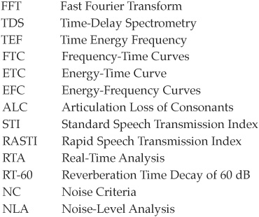
FFT, TDS, and TEF Measurement

While -octave analysis provides a wealth of information, it leaves out the very important ingredient of time. It will tell you what the frequency is and how much of it there is, but cannot tell you when it occurs. Temporal distribution or a sound’s place in time is important psychoacoustically. Time-delay spectrometry (TDS) can give you the levels of only the reflections, thus providing mathematical hints as to where they originated. Fast Fourier transform (FFT) transforms the time domain to frequency domain.

Let’s start with a bit of history. In the early 1960s, a scientist named Richard C. Heyser was working at the California Institute of Technology’s Jet Propulsion Laboratories. Jets were still new then; just ask any old-timer about the experimental aircraft like the X-15 and the test pilots who became our heroes as kids. Mr. Heyser was calibrating the frequency and phase response of an open-reel tape recorder and the time lag between the outputs of the two heads (record and reproduce) was giving him some trouble with his measurements. So he just went and assembled a bench-load of equipment to compensate for this offset in time. He found that his new test method not only corrected the time offset, but also canceled out the harmonic distortion. He realized he had something there and kept working on it, and described it in a 1967 AES paper.

Here’s my brief synopsis of a time energy frequency (TEF) test procedure as used when testing speakers. A sine-wave generator is used to produce the test signal that is fed through the monitor system, and a mic picks up the output from the speaker. In addition, the test system utilizes a tracking filter in sync with the generator and a delay module, which offsets the input timing, to correct for any delays incurred by the signal, such as propagation through air. The bandwidth and the time delay can be varied to allow for a test of only the direct sound, just the early reflections, or both. Even the earliest of these devices were quite informative to say the least. To say that they completely changed acoustic measurement would not be an exaggeration.

Due to the inherent noise rejection of TDS measurements, reverberation decay time can be calculated and displayed even when a high amount of background noise is present. TEF measurements can provide close to anechoic results in any room. A short time segment of a periodic signal can be sampled for a complete or whole number of periods, and from TDF the FFT can be extrapolated using one of the many “windowing” techniques available. This tiny little area of measurement has acronyms for days, so here’s a partial list that will help keep you somewhat afloat.

Back to some more history.

Mr. Cecil Cable picked up on the potential of this measurement procedure and in his 1977 AES paper, he described his research into comb filtering caused by early reflections. In 1979 Crown International (the amplifier manufacturer) began manufacturing their TEF system (a TDS analyzer in combination with FFT) that analyzed time, energy, and frequency. By 1980, Mr. Don Davis was not only teaching “Syn-Aud-Con” (synergetic audio concepts) students how to use a TEF device, but along with Chips Davis, designing and building control rooms based on the early reflection/comb-filtering information compiled by this system.

The resulting live end, dead end (LEDE) control room design had the psychoacoustic ability to make the control room boundaries seem to disappear from the listener’s perspective. The only way I can describe the one “true” LEDE control room I’ve had the opportunity to work in is that your perspective is not one of being in a control room listening to what is going on in the studio, but one of actually being in the studio listening to what is going on. The acoustics of the control room did not come between the listener and the sound. The maximum length sequence (MLS) of signals is used with FFT to provide frequency response, speech intelligibility, and time analysis. With random signals such as white or pink noise, the signal must be sampled over a period of time in order for the analyzer to generate accurate readings. A pseudorandom signal can be made up of a group of sounds that display any appropriate parameters needed to perform a specific test. This signal has a set length and is sequentially repeated.

Level versus frequency measurements are known to be an important indicator of a system’s capability to produce sound adequately, but time or phase versus frequency measurements are not given the same importance. In fact, many people feel that phase inconsistencies are inaudible. Mr. Heyser’s answer to this was to point out the fact that with a system’s low-frequency driver positioned relatively close to the listener and the high frequency driver placed a mile back, this system could actually achieve a flat frequency response if the high frequencies were driven with enough level. In this case, the phase response would give a better indication as to how bad it actually sounded. Beautiful response, no?

In source-independent measurement (SIM) FFT analysis, the input is fed to the analyzer and the system. The system’s output is then compared to the input signal. Thus, the test signal is “independent” of any restrictions except for being broadband in nature. Therefore, like the dbx RTA-1, it is possible to use music program for the test signal. Here the FFT’s “windowing” capabilities allow the operator to focus in on the test results down to a single cycle. By gating the input signal, different sections can be analyzed, and the display can show how frequencies change with time. Short gating times provide superior time resolution, and longer gating times give good frequency resolution. While a wealth of information is provided by the Neutrik 3000 strip chart recordings (see Fig. 3.2), the 3-D plots produced by these tools are no less than spectacular (see Fig. 3.3).

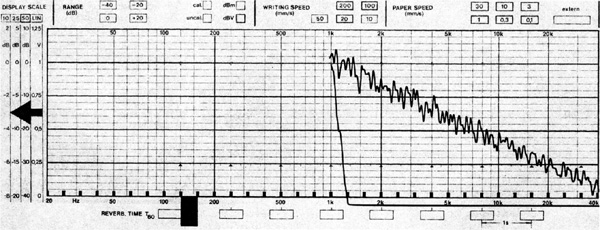
FIGURE 3.2 Neutrik Audiograph 3000 strip chart recording of the shortest and longest plate presets. Each vertical division equals of a second, which is also the shortest reverberation time. The longest is 5 full seconds!

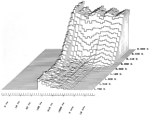
FIGURE 3.3 3-D level vs. frequency vs. time display. The only thing I remember about this 3-D plot is that I used it as an example when I taught at the Institute of Audio Research. But I can tell you that the horizontal and vertical planes are just the common level and frequency scales, but the “depth” is the time starting from 0 seconds at the back and ending at 1.750 seconds at the front. As you can see these plots provide a ton of information.