While we touched upon modern acoustic diffusers in Part I, in order to understand everything in the next section, a more thorough explanation is needed. One of the best basic explanations I know of was written by F. Alton Everest more than twenty five years ago. While there have been numerous advancements in this area, he not only clarified the need for diffusers but shed light on the theory behind their operation.
F. Alton Everest was a man of science. He held a B. Sc. (EE) degree from Oregon State University, an EE degree from Stanford University, and did graduate work in physics at the University of California/Los Angeles. Mr. Everest was involved in the early stages of television. He did underwater sound research during WW II and cofounded the Moody Institute in Los Angeles, where he was director of science and produced science films. He spent several years as senior lecturer on communications at the Hong Kong Baptist College in Hong Kong. He published many books and papers and was a member of SMPTE, ASA, Institute of Electrical and Electronic Engineers, and AES. He was cofounder and past president of the American Scientific Affiliation and is listed by American Men of Science.
It should be no surprise that he chose a scientific approach to unravel the mystery of diffusion. What follows represents some of what Mr. Everest had to say on the subject.
All that is required of the acoustical consultant is the design of studios and other rooms that engineers, musicians and the general public consider “good.” This is a difficult and subjective evaluation and the job definitely does not fall into the neat categories of definite black-white, go-no-go things of this world. If a room is too reverberant or too dead it is judged “bad” and adjusting reverberation within relatively close limits is probably the greatest single factor in elevating a poor room to a good or at least a better condition. However, reverberation time is not the only factor involved. Another factor is the diffusion of sound in the room. Often two studios very similar in size with the same reverberation time have a very different sound. This difference can possibly be traced to diffusion of sound in the room.
The relationship of diffusion of sound in a studio to the general acoustical quality of that studio is something of a mystery that has baffled studio designers for the last half century. What is diffusion? The sound field in a studio is diffuse if at any given instant the intensity of sound is uniform everywhere in that room and at every point sound energy flows equally in all directions. It has to do with homogeneity of sound in a room. Such a diffuse condition is a basic assumption in the derivation of the reverberation time equations of Sabine and Eyring. It is apparent that a dominant standing wave condition or knowledge that sound conditions vary throughout a studio means that a diffuse condition does not exist.
Diffusion is not the problem in large rooms such as auditoriums as it is in small rooms such as recording studios and listening rooms. This is the result of the fact that the dimensions of the smaller rooms are comparable to the wavelength of sound to be recorded or reproduced in them.
In Chapter 6 the effect of room size was considered along with room proportions. It was noted that the more uniform the distribution of room resonance modes the better. This procedure contributes to the diffusion of sound in the room. Selecting a cubical space in which all axial modes pile up at certain frequencies with great empty spaces between these pile-up frequencies is a move away from reasonably diffuse conditions. It is impossible, by traditional methods at least, to attain truly diffuse sound conditions in a small space, but approaching it as closely as possible is a major goal in studio design.
In the measurement of reverberation time the modes of the room are excited, say, with high intensity random noise from a loudspeaker. When the loudspeaker sound is suddenly terminated, these room modal frequencies die away, each at its own frequency and own rate.
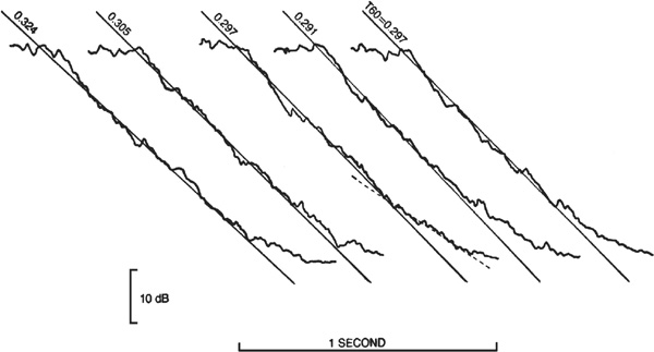
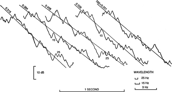
Figure 20.1 shows tracings from graphic level recorder records of five successive decays of an octave band of random noise centered at 125 Hz. The loudspeaker and microphone positions remained fixed. Figure 20.2 shows similar five successive decays under identical conditions except it is for an octave band of random noise centered on 4 kHz. The contrast in smoothness of decay is striking, yet these are typical of small studio decays at these frequencies. It is instructive to dig into this a bit further.
FIGURE 20.1 Graphic level recorder tracings of successive reverberatory decays under identical conditions of an octave band of random noise centered on 125 Hz. Evidence of beats between axial mode resonances is apparent.
FIGURE 20.2 Successive graphic level recorder tracings or decays under the same conditions as Fig. 20.1 except for an octave band centered on 4 kHz. An octave at this frequency contains so many modal frequencies that the decay is much smoother than an octave at 125 Hz. A second decay slope at low levels gives evidence of a slower rate of decay of certain room modes.
The 125 Hz and 4 kHz decays of Figs. 20.1 and 20.2 were made in a small multitrack studio 13 feet 5 inches × 18 feet 5 inches with a ceiling height of 7 feet 6 inches, volume 1,853 cubic feet. The object of the measurement was basically the determination of the reverberation time of the studio.
Establishing a best fit straight line average slope to the erratic decays at 125 Hz is far less precise than for the 4 kHz decays. To illustrate this, the squint-eye slope lines are included in Figs. 20.1 and 20.2 with the reverberation time (T60 seconds included at the top of each slope.
Of course, different observers establish slightly different slope fits, but the averaging of five slopes for each frequency and each microphone position gives a statistically significant mean value.
The mean value for the five 125 Hz decays for each of three microphone positions in this studio is 0.291 second with a standard deviation of 0.025 second. The same for the 4 kHz octave is 0.311 second with a standard deviation of 0.013 second. The standard deviation (the plus and minus deviations from the mean value which includes 67 percent of the measurements) for 125 Hz is twice that for 4 kHz which reflects the greater fluctuations in the 125 Hz measurements.
Of special interest in this chapter, the reverberation decays of Figs. 20.1 and 20.2 also reveal something of the sound diffusion conditions in this studio. Octave bands of random noise were used in both the 125 Hz and 4 kHz cases. An octave band centered on 125 Hz is considered to include energy from 88 to 177 Hz, the half-power (3 dB down) points. The 4 kHz octave covers 2,828 to 5,656 Hz, the one spanning 89 Hz, the other 2,828 Hz. The 125 Hz octave band includes relatively few modal frequencies of the room, the octave at 4 kHz many.
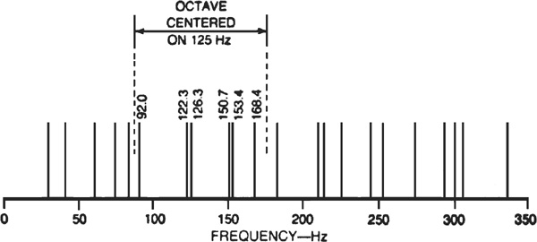
The axial mode frequencies for this small multitrack studio below 250 Hz are shown graphically in Fig. 20.3. Although there are no pile-ups several pairs are very close together and wide gaps (compared to the approximately 5 Hz bandwidth of each mode) occur.
FIGURE 20.3 The studio in which the decays of Figs. 20.1 and 20.2 were taken has axial modal frequencies as shown. The octave centered on 125 Hz passes only the six indicated. The close pairs within this octave tend to beat with each other causing fluctuations in the decay trace at the difference frequency.
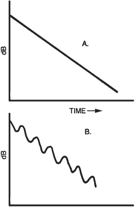
In Fig. 20.3 the span of the 125 Hz octave includes six modal frequencies. Each of these modes has its own decay rate determined by the absorption material in the room involved in that particular mode. A single mode, if excited and allowed to decay without influence of any other mode, would decay exponentially which gives a nice straight line decay on a dB scale as shown in Fig. 20.4A. The octave containing the six axial modes of Fig. 20.3 might be considered a combination of B and C, as seen in Fig. 20.1.
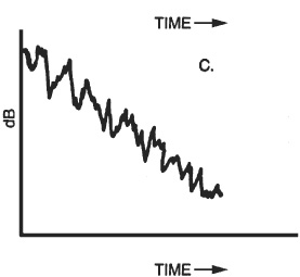
FIGURE 20.4 (A) A single mode decay exponentially, giving straight line decay on a logarithmic scale. (B) Two closely spaced modes, each having the same decay rate, beat with each other causing the decay to vary at the difference frequency. (C) Many closely spaced modes result in an erratic decay, the more modes the smoother the decay.
Then how is the smoothness of the decay curves of the 4 kHz octave (Fig. 20.2) explained? The 125 Hz octave is only 89 Hz wide while the octave centered on 4 kHz is 2,828 Hz wide. The greater smoothness is explained by the greater width and thus the greater number of modal frequencies included in the 4 kHz band. Only the axial modes are plotted in Fig. 20.3. It would be impossible to show graphically even the numerous axial modes within the 4 kHz octave, let alone the tangential and oblique modes. In fact, considering all three types of natural frequencies of this multitrack studio, something of the order of 800,000 modal frequencies exist in the 4 kHz octave band while only 328 exist in the 125 Hz octave band.
Of course, as pointed out in Chapter 6, the tangential and oblique modes have less influence than the axial, but they do have some effect and this effect would be in the direction of smoother decays and better diffusion.
The effect of difference beat frequencies between axial modes of Fig. 20.3 can be detected in the decays of Fig. 20.1. The graphic level recorder paper speed for both Figs. 20.1 and 2 was 100 mm per second and a one second scale is indicated on both of these figures. If the 153.4 Hz and the 168.4 Hz modes beat together, a difference frequency of 15 Hz is produced.
One cycle of a 15 Hz signal is represented by the length of the line so indicated in the lower right-hand corner of Fig. 20.1. In the second and fourth 125 Hz decays there are fluctuations closely matching this frequency. The 126.3 Hz and 150.7 Hz modes beating together would yield a difference beat frequency of 24.4 Hz.
There are fluctuations in decay one and three which are close to 25 Hz. The closely spaced modes near 125 Hz and 150 Hz (Fig. 20.3) produce beats of 3.6 and 2.7 Hz. Variations corresponding to the more slowly varying beats near 3 Hz are more difficult to pinpoint, but there are even suggestions of these. In other words, the modal frequencies within the 125 Hz octave band account for the relatively great fluctuations of the 125 Hz decays.
The reason the five decays are not identical or similar can be explained by the fact that the different modal frequencies were not all excited to the same level. The random noise signal constantly changes in amplitude and frequency (within the octave limits). It is entirely fortuitous as to what instantaneous amplitude and frequency were at the time the sound was interrupted to begin the decay. A very smooth low frequency decay could result from a dominant single mode, although with octave bands this is unlikely.
An important indication of the diffusion of sound in this small multitrack studio is given in the low frequency reverberation decays as in Fig. 20.1. If the fluctuations are very great, the diffusion is poor. The smoother the decays, the better the diffusion.
Quantitative evaluation of diffusion conditions are not yet available from such decays, but good qualitative comparisons are not only possible, but part of the arsenal of informed workers in studios.
Diffusion information may also be gleaned from decay curves at higher frequencies. In Fig. 20.2 the broken line indicates a fairly definite suggestion of a second slope. This is probably the result of certain modal frequencies having less contact with the absorbing material in the room (i.e., modes that are less damped) or modal frequencies not fully excited as the decay begins. In this particular case, these modes do not affect things until the sound has decayed 30 dB, hence their effect would probably not be detectable in normal program material.
Measuring reverberation time at different locations in a studio often reveals small but significant differences in reverberation time. These are usually averaged together for a better statistical description of conditions in the studio.
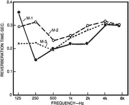
For example, Fig. 20.5 shows the reverberation time measured at three different microphone positions in the small multitrack studio mentioned in the previous section. It is noticed that the three graphs tend to draw together as frequency is increased. This suggests that such changes in reverberation time at different locations in the same studio are the result of a certain degree of nondiffuse conditions because we know that diffusion is better at high frequencies. Can this method then be used to evaluate the sound diffusion condition in a room?
FIGURE 20.5 Variation of reverberation time/frequency graphs with position in a small studio. The modal content of the octaves at different frequencies varies, and the decay rate of the different modes varies. To obtain a statistical picture of the sound field in the room, it is customary to average the measured reverberation times for each frequency at each position.
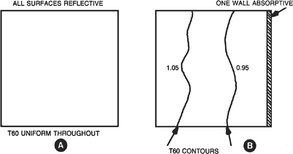
The Engineering Research Department of the British Broadcasting Corporation asked the same question.33 In their characteristically thorough way they measured reverberation time at 100 microphone positions in a 10-foot × 10-foot room. With no absorption material in the room (Fig. 20.6A), very diffuse conditions resulted in reverberation time long, but essentially constant throughout the room.
FIGURE 20.6 (A) If all surfaces of a room are 100 percent reflective, the sound field is completely diffuse and the decay rate is the same at every point in the room. (B) If one wall is absorptive, the decay rate varies from point to point in the room. The contours of decay rate tend to be parallel to the treated wall.
In Fig. 20.6B the reverberation time contours are shown when one wall was treated. The reverberation time is lower nearer the absorbing surface. They then demonstrated that geometrical diffusing elements on the untreated walls plus one absorbing wall resulted in quite complex contours. The laborious nature of this approach discourages further exploration of the method, although it shows some promise if special instrumentation were devised.
The signal output of a highly directional microphone in a perfectly diffuse room should be the same no matter where it is pointed, except when pointed at the source of sound. Ribbon microphones, with their figure-8 pattern, have been tried. Parabolic reflectors with a microphone at the focal point have been tried, as well as the line array type of directional microphone.
All of these methods have proved to be rather awkward to use and the results difficult to interpret. The greatest shortcoming of this method, from the point of view of small studios, is that sharp microphone directivity is hard to get at the low frequencies at which diffusion is the greatest problem. The prospect of this method of appraising diffusion in small studios is poor.
For the last half century there have been many serious efforts to evaluate diffusion in rooms by steady-state transmission measurements.34,36 Microphone and loudspeaker positions remain fixed. The constant amplitude swept sine wave signal radiated from the loudspeaker and picked up by the microphone has the room effect impressed upon it. This room influence should reveal something about the room.
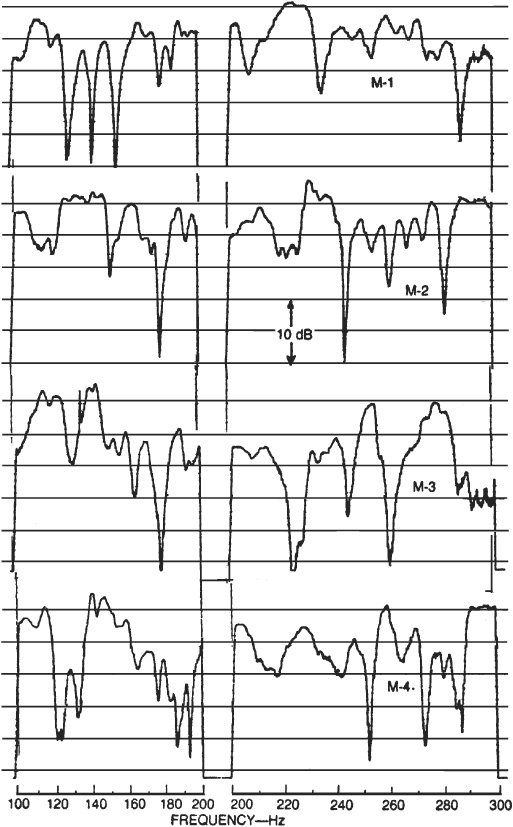
Figure 20.7 shows typical frequency response records taken in a music studio of 16,000 cubic foot volume having a reverberation time of about 0.6 second at the 100–300 Hz frequency region under investigation. Two things are very striking:
FIGURE 20.7 Typical steady state swept sine frequency response records taken at different positions in a music recording studio having a volume of 16,000 cubic feet and a reverberation time of 0.6 second. The striking variations are an indication that even a well-treated studio falls far short of truly diffuse conditions. At frequencies above 300 Hz, the curves becomes progressively smoother.
• The magnitude of the variations
• The differences from position to position in the room
The amazing thing is that fluctuations in point-to-point response of such magnitude occur in studios having the best acoustical treatment and those considered excellent in subjective evaluations. The loudspeaker response in the 100–300 Hz region is included in these recordings, but it remains constant through all the tests.
If such wild fluctuations are to be of any help in evaluating studios, it is necessary to find some method of reducing them to numbers. Bolt has suggested the term frequency irregularity factor obtained by adding all the peak levels, subtracting the sum of all the corresponding dip levels, and dividing the difference dB by the number of hertz swept. This frequency irregularity factor, or simply FI factor, is in dB/Hz.
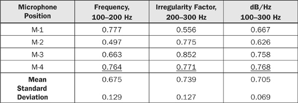
Applying this procedure to Fig. 20.7 yields the FI factors tabulated in Table 20.1. Comparison of Fl factors for the different microphone positions would seem to tell us that conditions at M-2 are the best, considering the 100–300 Hz range, and that M-1 and M-2 are superior to M-3 and M-4.
TABLE 20.1 Frequency Irregularity
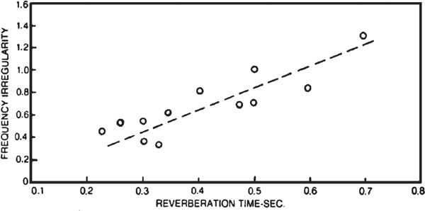
Glancing back to Fig. 20.7 would seem to support this. What the FI factors of Table 20.1 tell us about sound diffusion in the room is not so clear. In measuring many studios it was noticed that larger FI factors were commonly associated with longer reverberation times. The 100–300 Hz FI factor for a dozen studios is plotted in Fig. 20.8 against their corresponding reverberation times. The broken line (not a least-squares fit) would seem to indicate a definite relationship.
FIGURE 20.8 The variation of measured frequency irregularity factor with studio reverberation time.
In fact, theoretical studies and experimental results have shown that at high frequencies frequency irregularity is related only to reverberation time and that it gives no additional information on diffusion of sound in the room. Whether or not this is true in the 100–300 Hz region remains to be seen.
One thing seems to be clear, if at a certain microphone position the swept frequency response is within, say, ±5 dB, that would be a good spot for a narrator to sit.
A corollary to that observation is that it is possible to compare microphone positions by a swept frequency signal test. For such a test a good place for the loudspeaker would be in a corner of the room. If standing waves such as indicated by the runs of Fig. 20.7 exist in what are called well-treated studios, conditions may be less bad in some spots than in others. This is of operational value only if recording in a studio can be done with a single microphone in a fixed position.
A minimum studio or control room volume of 1,500 cubic feet has been urged. This is step one toward better diffusion. Rooms smaller than this are often plagued with coloration problems, impossible or impractical to correct. Of course, rooms having substantially greater volumes but still in the general small room category have plenty of diffusion problems also, but the chances of achieving satisfactory conditions by the application of the methods to be described are better.
By making a room large in terms of the wavelength of the sound to be recorded in it means that the modal frequencies will be closer together which means improved diffusion. Most of the methods of diffusing sound in a room to be considered later are most effective at the higher audio frequencies. Optimizing the proportions of the room is one of the most effective ways to improve diffusion at the low end of the audible band. There are a number of steps in the acoustical treatment of a room which tend toward better diffusion of sound in the room, once the major basic matter of room size and proportions are set (review Chapter 6 in this regard).
Numerous controlled experiments and practical experience have demonstrated that concentrating the required absorbing material on one or two surfaces of a room is an acoustical abomination. Common sense emphasizes that this procedure often leaves some opposing or parallel walls untreated, producing some axial resonances.
The application of absorbing material in patches has been established as far superior to application in fewer large areas. This accounts for the proliferation of wall modules and sectionalized ceilings in studio designs in this book. The patches of absorbing material may be distributed by determining the areas of the N-S, E-W, and vertical pairs of surfaces and dividing the material between the three axial modes proportionally. At least, this is a respectable criterion to use as a rough guide, even though practical considerations like doors, observation windows, and floor coverings demand compromise.
Another important contribution of patches of absorbing material is that diffraction of sound, especially at the higher frequencies, takes place at the edges of each patch. Such diffraction contributes helpfully to diffusion. Placing absorbent where it acts on every axial, tangential and oblique mode is smart, remembering that all modes terminate in corners. Distributing absorbent in patches contributes to absorption efficiency as well as diffusion. Diffraction effects act as though the absorbent “sucks” sound energy from the surrounding reflective area which, in effect, increases its absorption coefficient.
The conventional wisdom among studio people has long held that splayed walls aid in diffusion of sound. Splayed walls do have the ability to help in the control of flutter echoes between opposite reflective surfaces, but do they really contribute significantly to diffusion? Model experiments have shown that the frequency irregularity factor is reduced with walls canted 5 percent but there is some question of this applying to practical studios with less smooth walls. The BBC made subjective tests in which experienced listeners listened with and without splayed walls with patches of absorbent on them and the results were inconclusive.
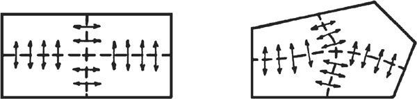
Rectangular and trapezoidal room shapes are illustrated in Fig. 20.9. The broken lines represent the sound pressure modal contours for a simple mode for both shapes. The small arrows represent the directions of particle motion in the two cases. The trapezoidal room shape most certainly has contributed something to diffusion, but the magnitude of the contribution is small for walls splayed the usual one part in 10.
FIGURE 20.9 The broken lines indicate the sound pressure modal contours for a simple mode in rectangular and trapezoidal rooms. The small arrows represent the direction of particle motion. It is obvious that the trapezoidal room shape contributes something to diffusion.
It appears that justification of splayed walls must come from reduction of flutter echoes rather than improvement of diffusion. As there are other ways to prevent flutter echoes (such as patches of absorbent) it would seem that tearing an existing building apart to cant walls might be ill-advised. In new construction, however, inclining the walls might cost very little.
In low frequency Helmholtz resonators, what happens to incident sound energy that is not absorbed by the system? It is scattered and scattering contributes to diffusion of sound energy in the room. This is not true of the porous type of absorbers in which energy not absorbed is reflected from the backing surface. Remember, however, that high frequency energy not affected by a perforated or slat low frequency absorber can be reflected and contribute to a flutter echo problem. This would suggest facing such units with a high frequency absorber or inclining its surface.
There have been numerous, and presumably effective, geometrical protuberances employed in studios to diffuse sound. Common among these are semicylindrical (poly) diffusers37 and diffusers of rectangular and triangular cross section. The polycylindrical surface has been widely applied in studios, not only for its low frequency absorption, but for its ability to take sound arriving from a given direction and reradiate it through an angle of 100 degrees to 120 degrees. This contributes positively to diffusion in the room.
In spite of the salutary effect of polycylindrical elements, both controlled experiments38 and theoretical studies39 have demonstrated the marked superiority of rectangular protrusions over both cylindrical and triangular. The rectangular protrusions produce some effect when their depth is as shallow as one-seventh of the wavelength. Thus a rectangular element 6-inches deep has some effect down to approximately 325 Hz. This effect works to change the normal modes of a smooth-walled room. The cylindrical and triangular projections also do this, but to a lesser degree.
The acoustical distinguishing feature that sets the rectangular apart is the fact that it has finite portions perpendicular to the wall on which it is mounted. It has the ability of breaking up concentrations of modal frequencies better than cylindrical or triangular protrusions, of reducing the magnitude of dominant modes, and lowering the frequency irregularity in swept sine transmission. This provides some support for the proliferation of the not-too-beautiful wall modules in studio designs already considered.
Other diffusing elements found in every studio, control room, and listening room are people, tables, chairs, door and window frames, and equipment of every sort.
The optical diffraction grating can break down a beam of sunlight into all the colors of the rainbow. The type of grating used in optical studies has microscopically fine, parallel lines ruled on glass. Inexpensive plastic replicas are available as toys and the principle is applied in colorful advertising signs.
What has this to do with acoustics? Dr. Manfred Schroeder of the AT&T Bell Laboratories has made the connection in a very positive way.44 Imagine a surface with a series of long, narrow, parallel wells, or grooves, on it. The wells are of either fixed or of varying depth, but of constant width. A sound ray impinging on this surface finds itself interacting with reflections from the bottoms of the wells. The phase (or time relationship) of the reflections from the wells varies with the depth of the wells; hence the arriving sound ray must interact with well reflections delayed varying amounts. Dr. Schroeder related the well depths to various mathematical sequences 45 which result in sound coming from a given direction to be scattered throughout 180 degrees. In this way mysterious mathematical names have come to identify different types of these diffusers: quadratic residue sequence, primitive root sequence, maximum length sequence, etc. They all scatter sound better than what was available in the past, but some are more efficient for specific tasks than others.
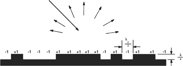
Figure 20.10 shows a specific type of diffraction grating sound diffuser, the kind Dr. Schroeder first tried. He needed different reflection coefficients of + and −1. A groove a quarter wavelength deep gives a reflection coefficient of −1 while no groove at all gives a reflection coefficient of + 1. This emphasizes that a design frequency must first be selected. Let us take 1000 Hz as our design frequency. The wavelength of a 1000 Hz tone is 13.56 inches, a half wavelength is 6.68 inches, and a quarter wavelength is 3.39 inches. As shown in Fig. 20.10 the well depth must then be 3.39 inches and the unit well width 6.78 inches. It can be made of wood, metal, or plastic or any other substance which is a good reflector of sound. The question now is, “Will it diffuse only 1000 Hz sound?” This maximum length sequence diffuser will work well over about one octave, a half octave above and a half octave below 1000 Hz. The diffused energy is confined to a hemidisk at right angles to the face of the diffuser.
FIGURE 20.10 A diffusing surface based on a maximum length sequence. The grooves of quarter wavelength depth offer a reflection coefficient of –1, the high spots +1. Good diffusion a half octave above and below the design frequency is realized.
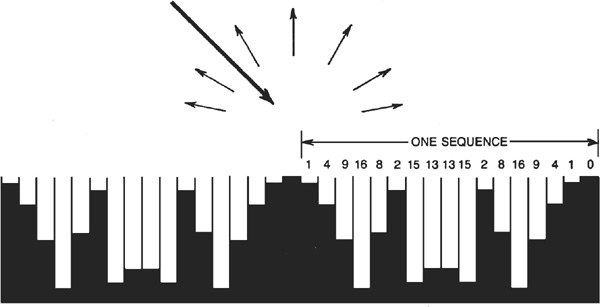
The more complex grating diffusers perform much better. A quadratic residue diffuser is shown in Fig. 20.11. Here the sequence length is 17 and the relative well depths are as indicated and shown graphically. Two sequences are shown in the figure. Thin metal separators maintain the identity of each well. The width of the wells is about a half wavelength at the shortest wavelength to be scattered effectively. The maximum well depth is determined by the longest wavelength to be diffused. Although more difficult to construct, quadratic residue diffusers scatter sound effectively over most of the audible band.
FIGURE 20.11 A diffusing surface based on a quadratic residue sequence. Good diffusion over most of the audible band can be achieved with this type of diffuser.
In the past the designer and builder of a studio, control room, or listening room had only reflection and absorption to work with; diffusion was largely out of reach. That has now changed. Standard diffusing units are now commercially available Such units are being installed in recording studios and control rooms as well as concert halls, churches, and home listening rooms.
Diffraction grating sound diffusers are also being applied in small budget recording facilities. They are not a cure-all for the acoustical problems of small rooms but they do add a new tool to the designer’s toolbox.
Are the principles elucidated in earlier chapters of this book outdated by the coming of effective diffusing elements? Not at all, but the prospects of better sound from small rooms are much improved.46-53
NOTE: If this explanation is not technical enough, you can download Dr. Manfred Schroeder’s original J. Acoust. Soc. Am. April 1979 paper titled “Binaural Dissimilarity and Optimum ceilings for Concert Halls” or get the full deal by purchasing Acoustic Absorbers and Diffusers, Theory, Design and Application by Trevor J. Cox and Peter D’Antonio.