Chapter 6: Using Lookup Formulas
Finding data in a list or table is central to many Excel formulas. Excel provides several functions to assist in looking up data vertically, horizontally, from left to right, and from right to left. By nesting some of these functions, you can write a formula that looks up the correct data even after the layout of your table changes.
 You can download the files for all the formulas at www.wiley.com/go/101excelformula.
Formula 55: Looking Up an Exact Value Based on a Left Lookup Column
Many tables are arranged so that the key piece of data, the data that makes a certain row unique, is in the far-left column. Although Excel has many lookup functions, VLOOKUP was designed for just that situation. Figure 6-1 shows a table of employees. You want to fill out a simplified paystub form by pulling the information from this table when an employee’s ID is selected.
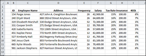
Figure 6-1: A table of employee information.
The user will select an employee ID from a data validation list in cell L3. From that piece of data, the employee’s name, address, and other information will be pulled into the form. The formulas for the paystub form in Figure 6-2 are shown here:
Employee Name: =VLOOKUP($L$3,$B$3:$I$12,2,FALSE)
Pay: =VLOOKUP($L$3,$B$3:$I$12,5,FALSE)/VLOOKUP($L$3,$B$3:$I$12,4,FALSE)
Taxes: =(M7-O8-O9)*VLOOKUP($L$3,$B$3:$I$12,6,FALSE)
Insurance: =VLOOKUP($L$3,$B$3:$I$12,7,FALSE)
Retirement: =M7*VLOOKUP($L$3,$B$3:$I$12,8,FALSE)
Total: =SUM(O7:O10)
Net Pay: =M7-O11
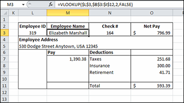
Figure 6-2: A simplified paystub form.
How it works
The formula to retrieve the employee’s name uses the VLOOKUP function. VLOOKUP takes four arguments: lookup value, lookup range, column, and match. VLOOKUP searches down the first column of the lookup range until it finds the lookup value. When the lookup value is found, VLOOKUP returns the value in the column identified by the column argument. In this case, the column argument is 2, and VLOOKUP returns the employee’s name from the second column.
All of the VLOOKUP functions in this example have FALSE as the final argument. A FALSE in the match argument tells VLOOKUP to return a value only if it finds an exact match. If it doesn’t find an exact match, VLOOKUP returns N/A#. Formula 60, later in this chapter, shows an example of using TRUE to get an approximate match.
The other formulas also use VLOOKUP with a few twists. The address and insurance formulas work just like the employee name formula, but they pull from a different column. The pay formula uses two VLOOKUPs; one divided by the other. The employee’s annual pay is pulled from the fifth column and is divided by the frequency from the fourth column, resulting in the pay for one paystub.
The retirement formula pulls the percentage from the eighth column and multiplies that by the gross pay to calculate the deduction. Finally, the taxes formula deducts both insurance and retirement from gross pay and multiplies that by the tax rate, found with VLOOKUP pulling from the sixth column.
Of course, payroll calculations are a little more complex than this, but when you understand how VLOOKUP works, you can build ever more complex models.
Formula 56: Looking Up an Exact Value Based on Any Lookup Column
Unlike the table used in Formula 55, not all tables have the value you want to look up in the leftmost column. Fortunately, Excel provides some functions for returning values that are to the left of the value you’re looking up.
Figure 6-3 shows a list of cities and states where the stores are. You want to return the city and store number when the user selects the state from a drop-down box.
City: =INDEX(B3:D25,MATCH(G4,C3:C25,FALSE),1)
Store: =INDEX(B3:D25,MATCH(G4,C3:C25,FALSE),3)
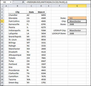
Figure 6-3: A list of stores with their city and state.
How it works
The INDEX function returns the value from a particular row and column of a range. In this case, you pass it your table of stores, a row argument in the form of a MATCH function, and a column number. For the City formula, you want the first column, so the column argument is 1. For the Store formula, you want the third column, so the column argument is 3.
Unless the range you use starts in A1, the row and column won’t match the row and column in the spreadsheet. They relate to the top, left cell in the range, not the spreadsheet as a whole. A formula like =INDEX(G2:P10,2,2) would return H3. The cell H3 is in the second row and the second column of the range G2:P10.
 The second argument of the MATCH function can be only a range that is one row tall or one column wide. If you send it a range that’s a rectangle, MATCH returns the #N/A error.
To get the correct row, you use a MATCH function. The MATCH function returns the position in the list where the lookup value is found. It has three arguments:
- Lookup value: The value you want to find.
- Lookup array: The single column or single row to look in.
- Match type: For exact matches only, set this argument to FALSE or 0.
The value you want to match is the state in cell G4, and you’re looking for it in the range C3:C25, the list of states. MATCH looks down the range until it finds "NH". It finds it in the 12th position, so 12 is used by INDEX as the row argument.
With MATCH computed, INDEX now has all it needs to return the right value. It goes to the 12th row of the range and either gets the value from the first column (for City) or the third column (for Store #).
If you pass INDEX a row number that is more rows than is in the range or a column number that is more columns, INDEX returns the #REF! error.
Alternative: The LOOKUP function
Although VLOOKUP is the most popular lookup function, the combination of INDEX and MATCH is a close second. A lesser-used alternative is the LOOKUP function. LOOKUP takes these three arguments:
- Lookup value: The value you want to find
- Lookup vector: The single column or single row to look in
- Results vector: The single column or single row to return from
The following formulas are for finding the City and Store # from Figure 6-3:
City: =LOOKUP(G4,C3:C25,B3:B25)
Store: =LOOKUP(G4,C3:C25,D3:D25)
The first two arguments of LOOKUP are identical to the first two arguments of MATCH. In fact, LOOKUP works similarly to MATCH in that it finds the position of the lookup value in the lookup vector. Rather than returning that position, however, it returns the value in the same position within the results vector.
To find the city, LOOKUP calculates that "NH" is in the 12th position of the lookup vector (C3:C25) and returns the value in the 12th position of the results vector (B3:B25).
Formula 57: Looking Up Values Horizontally
If the data is structured in such a way that your lookup value is in the top row rather than the first column and you want to look down the rows for data rather than across the columns, Excel has a function just for you.
Figure 6-4 shows a table of cities and their temperatures. The user will select a city from a drop-down box, and you want to return the temperate to the cell just below it.
=HLOOKUP(C5,C2:L3,2,FALSE)
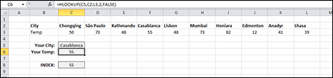
Figure 6-4: A table of cities and temperatures.
How it works
The HLOOKUP function has the same arguments as VLOOKUP. The H in HLOOKUP stands for horizontal, and the V in VLOOKUP stands for vertical. Instead of looking down the first column for the lookup_value argument, HLOOKUP looks across the first row. When it finds a match, it returns the value from the second row of the matching column.
Alternative
HLOOKUP and VLOOKUP are very similar functions. Just as you can substitute a combination of INDEX and MATCH for VLOOKUP, so can you for HLOOKUP.
=INDEX(C2:L3,2,MATCH(C5,C2:L2,FALSE))
In this case, the row argument of INDEX is hardcoded to “2”, and the MATCH function feeds the column argument. MATCH can look at single rows of values as well as single columns. As before, it returns the position of the matched item.
Formula 58: Hiding Errors Returned by Lookup Functions
So far, you’ve used FALSE for the last argument of your lookup functions so that you return only exact matches. When you force a lookup function to return an exact match but it can’t find one, it returns the #N/A error.
The #N/A error is useful in Excel models because it alerts you when a match couldn’t be found. But you may be using all or a portion of your model for reporting, and #N/A errors are ugly. Excel has functions to see those errors and return something different.
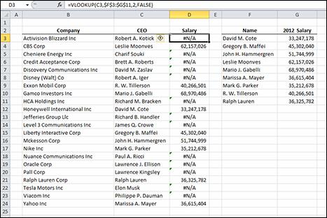
Figure 6-5: A report of CEO salaries.
Figure 6-5 shows a list of companies and CEOs. The other list shows CEOs and salaries. A VLOOKUP function is used to combine the two tables. But you obviously don’t have salary information for all of the CEOs, and you have a lot of #N/A errors.
=VLOOKUP(C3,$F$3:$G$11,2,FALSE)
In Figure 6-6, the formula has been changed to use the IFERROR function to return a blank if no information is available. The IFERROR function is known as an error trapping function because it recognizes, or traps, errors and provides a way for you to handle them other than simply allowing them to propagate through your formula.
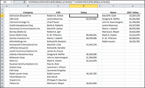
Figure 6-6: A cleaner report.
=IFERROR(VLOOKUP(C3,$F$3:$G$11,2,FALSE),"")
How it works
The IFERROR function accepts a value or formula for its first argument and an alternative return value for its second argument. When the first argument returns an error, the second argument is returned. When the first argument is not an error, the results of the first argument are returned.
In this example, you’ve made your alternative return value an empty string (two double quotation marks with nothing between them). That keeps the report nice and clean. But you could return anything you want, such as “No info” or 0.
The IFERROR checks for every error that Excel can return, including #N/A, #DIV/0!, and #VALUE. You can’t restrict which errors IFERROR catches or ignores and that can hide errors that you otherwise would not want to hide.
Excel provides three other error-trapping functions: ISERROR returns TRUE if its argument returns any error; ISERR returns TRUE if its argument returns any error except #N/A; ISNA returns TRUE if its argument returns #N/A and returns FALSE for anything else include other errors.
All these error-trapping functions return either TRUE or FALSE and are most commonly used with an IF function.
Alternative: The ISNA Function
IFERROR was introduced in Excel 2010. In older versions, you can use the ISNA function to check for errors.
=IF(ISNA(VLOOKUP(C3,$F$3:$G$11,2,FALSE)),"",VLOOKUP(C3,$F$3:$G$11,2,FALSE))
The ISNA function returns TRUE if its argument returns the #N/A error and returns FALSE if it doesn’t. The IF function checks for the error, returns an empty string if it’s there, or returns the value of the VLOOKUP if it’s not.
The downside to using ISNA is that you have to include the formula twice: once inside ISNA and once for the third argument of the IF function. This means that Excel has to calculate the same formula twice, and if you have a calculation-intensive workbook, it will be even slower.
Formula 59: Finding the Closest Match from a List of Banded Values
The VLOOKUP, HLOOKUP, and MATCH functions allow the data to be sorted in any order when you want an exact match. You set each of their final arguments to FALSE to force an exact match or to return an error.
These functions also work on sorted data for the times you want only an approximate match. Figure 6-7 shows a method for calculating income tax withholding. The withholding table doesn’t have every possible value, but it has bands of values. You first determine which band the employee’s pay falls in, and then you use the information on that row to compute the withholding:
=VLOOKUP(D15,B3:E10,3,TRUE)+(D15-VLOOKUP(D15,B3:E10,1,TRUE))*VLOOKUP(D15,B3:E10,4,TRUE)
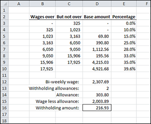
Figure 6-7: Computing income tax withholding.
How it works
The formula uses three VLOOKUP functions to get three pieces of data from the table. The final argument for each VLOOKUP formula is TRUE, indicating you want only an approximate match.
To get a correct result when using a final argument of TRUE, the data in the lookup column (column B in Figure 6-7) must be sorted lowest to highest. VLOOKUP looks down the first column and stops when the next value is higher than the lookup value. In that way, it finds the largest value that is not larger than the lookup value.
 Finding an approximate match with a lookup function does not find the closest match. Rather, it finds the largest match that’s not larger than the lookup value even if the next highest value is closer to the lookup value.
If the data in the lookup column isn’t sorted highest to lowest, you may not get an error, but you will likely get an incorrect result. The lookup functions use a binary search to find an approximate match. A binary search basically starts in the middle of the lookup column and determines whether the match will be in the first half or the second half of the values. Then it splits that half in the middle and looks either forward or backward depending on the middle value. That process is repeated until the result is found.
You can see with a binary search that unsorted values could cause the lookup function to choose the wrong half to look in and return bad data.
In the example in Figure 6-7, VLOOKUP stops at row 5 because 1,023 is the largest value in the list that’s not larger than the lookup value of 2,003.89. The three sections of the formula work as follows:
- The first VLOOKUP returns the base amount in the third column, or 69.80.
- The second VLOOKUP subtracts the “Wages over” amount (from the first column) from the total wages.
- The last VLOOKUP returns the percentage in the fourth column. This percentage is multiplied by the excess wages, and the result is added to the base amount.
When all three VLOOKUP functions are evaluated, the formula computes, as shown here:
=69.80 + (2,003.89 - 1,023.00) * 15.0%
The method the lookup functions use to find an approximate match is much faster than an exact match. For an exact match, the function has to look at every single value in the lookup column. If you know your data will always be sorted lowest to highest and will always contain an exact match, you can decrease calculation time by setting the last argument to TRUE. An approximate match lookup will always find an exact match if it exists and if the data is sorted.
Alternative: INDEX and MATCH
As with all of your lookup formulas, the INDEX and MATCH combination can be substituted. As do VLOOKUP and HLOOKUP, MATCH has a final argument to find approximate matches. MATCH has the added advantage of being able to work with data that is sorted highest to lowest.
Figure 6-8 shows the same withholding table as Figure 6-7 except that the data is sorted in descending order. The VLOOKUP based formula from Figure 6-7 returns #N/A, as shown in cell D16 on Figure 6-8. This is because VLOOKUP looks at the middle of the lookup column, determines that it is higher than the lookup value, and then looks only at values before the middle value. Because your data is sorted descending, no values before the middle value are lower than the lookup value.
The INDEX and MATCH formula in cell D18 of Figure 6-8 returns the correct result and is shown here:
=INDEX(B3:E10,MATCH(D15,B3:B10,-1)+1,3)+(D15-INDEX(B3:E10,MATCH(D15,B3:B10,-1)+1,1))*INDEX(B3:E10,MATCH(D15,B3:B10,-1)+1,4)
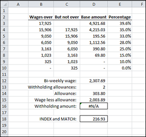
Figure 6-8: Calculating withholding using INDEX and MATCH.
The final argument of MATCH can be –1, 0, or 1.
- –1 is used for data that is sorted highest to lowest. It finds the smallest value in the lookup column that is larger than the lookup value. There is not an equivalent method using VLOOKUP or HLOOKUP.
- 0 is used for unsorted data to find the exact match. It is equivalent to setting the final argument of VLOOKUP or HLOOKUP to FALSE.
- 1 is used for data that is sorted lowest to highest. It finds the largest value in the lookup column that is smaller than the lookup value. It is equivalent to setting the final argument of VLOOKUP or HLOOKUP to TRUE.
Because MATCH with a final argument of –1 finds a value that is larger than the lookup value, the formula adds 1 to the result to get the proper row.
Formula 60: Looking Up Values from Multiple Tables
Sometimes the data you want to look up can come from more than one table, depending on a choice that the user makes. In Figure 6-9, a withholding calculation similar to Formula 59 is shown. The difference is that the user can select whether the employee is single or married. If the user chooses Single, the data is looked up in the Single Person table; if the user chooses Married, the data is looked up in the Married Person table.
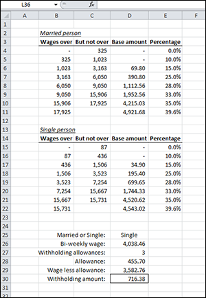
Figure 6-9: Computing income tax withholding from two tables.
In Excel, you can use named ranges and the INDIRECT function to direct your lookup to the appropriate table. Before you can write the formula, you need to name two ranges: Married for the Married Person table and Single for the Single Person table. Follow these steps to create the named ranges:
- Select the range B4:E11.
- Click the Define Name button found on the Formulas tab on the Ribbon. The New Name dialog box shown in Figure 6-10 is displayed.
- Change the Name text box to Married.
- Click OK.
- Select the range B15:E22.
- Click the Define Name button found on the Formulas tab on the Ribbon.
- Change the Name text box to Single.
- Click OK.
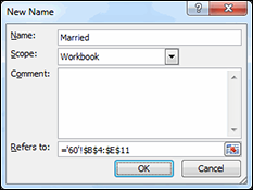
Figure 6-10: The New Name dialog box.
There is a data validation drop-down box in cell D25 in Figure 6-9. The drop-down box contains the terms Married and Single, which are identical to the names you just created. You use the value in D25 to determine which table to look in, so the values must be identical.
Here’s the revised formula for computing the withholding:
=VLOOKUP(D29,INDIRECT(D25),3,TRUE)+(D29-VLOOKUP(D29,INDIRECT(D25),1,TRUE))*VLOOKUP(D29,INDIRECT(D25),4,TRUE)
How it works
The formula in this example is strikingly similar to Formula 59. The only difference is that you use an INDIRECT function in place of the table’s location.
INDIRECT takes an argument named ref_text. The ref_text argument is a text representation of a cell reference or a named range. In Figure 6-9, cell D25 contains the text Single. INDIRECT attempts to convert that into a cell or range reference. If ref_text is not a valid range reference (as in this case), INDIRECT checks the named ranges to see whether a match exists. Had you not already created a range named Single, INDIRECT would return the #REF! error.
INDIRECT has a second optional argument named a1. The a1 argument is TRUE if ref_text is in the A1 style of cell references and FALSE if ref_text is in the R1C1 style of cell references. For named ranges, a1 can be either TRUE or FALSE, and INDIRECT will return the correct range.
INDIRECT can also return ranges from other worksheets or even other workbooks. However, if it references another workbook, that workbook must be open. INDIRECT doesn’t work on closed workbooks.
Formula 61: Looking Up a Value Based on a Two-Way Matrix
A two-way matrix is a rectangular range of cells. That is, it’s a range with more than one row and more than one column. In other formulas, you’ve used the INDEX and MATCH combination as an alternative to some of the lookup functions. However, INDEX and MATCH were made for two-way matrixes.
Figure 6-11 shows a table of sales figures by region and year. Each row represents a region and each column represents a year. You want the user to select a region and a year and return the sales figure at the intersection of that row and column.
=INDEX(C4:F9,MATCH(C13,B4:B9,FALSE),MATCH(C14,C3:F3,FALSE))
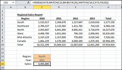
Figure 6-11: Sales data by region and year.
How it works
By now, you’re no doubt familiar with INDEX and MATCH. Unlike other formulas, you’re using two MATCH functions within the INDEX function. The second MATCH function returns the column argument of INDEX as opposed to hardcoding a column number.
Recall that MATCH returns the position in a list of the matched value. In Figure 6-11, the North region is matched, so MATCH returns 3 because it’s the third item in the list. That becomes the row argument for INDEX. The year 2011 is matched across the header row, and because 2011 is the second item, MATCH returns 2. INDEX then takes the 2 and 3 returned by the MATCH functions to return the proper value.
Alternative: Using default values for MATCH
To add a twist to your sales lookup formula, you change the formula to allow the user to select only a region, only a year, or neither. If one of the selections is omitted, you assume that the user wants the total. If neither is selected, you return the total for the whole table.
=INDEX(C4:G10,IFERROR(MATCH(C13,B4:B10,FALSE),COUNTA(B4:B10)),IFERROR(MATCH(C14,C3:G3,FALSE),COUNTA(C3:G3)))
The overall structure of the formula is the same, but a few details have changed. The range for INDEX now includes row 10 and column G. Each MATCH function’s range is also extended. Finally, both MATCH functions are surrounded by an IFERROR function that will return the Total row or column.
The alternative value for IFERROR is a COUNTA function. COUNTA counts both numbers and text and, in effect, returns the position of the last row or column in your range. You could have hardcoded those values, but if you happen to insert a row or column, COUNTA adjusts to always return the last one.
Figure 6-12 shows the same sales table, but the user has left the Year input blank. Because the column headers have no blanks, MATCH returns #N/A. When it encounters that error, IFERROR passes control to the value_if_error argument, and the last column is passed to INDEX.
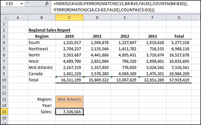
Figure 6-12: Returning totals from the sales data.
Formula 62: Finding a Value Based on Multiple Criteria
Figure 6-13 shows a table of departmental budgets. When the user selects a region and department, you want a formula to return the budget. You can’t use VLOOKUP for this formula, because it accepts only one lookup value. You need two lookup values because the regions and departments appear multiple times.
 See Chapter 5 for a discussion of how SUMPRODUCT uses arrays.
You can use the SUMPRODUCT function to get the row that contains both lookup values.
=SUMPRODUCT(($B$3:$B$45=H5)*($C$3:$C$45=H6)*($E$3:$E$45))
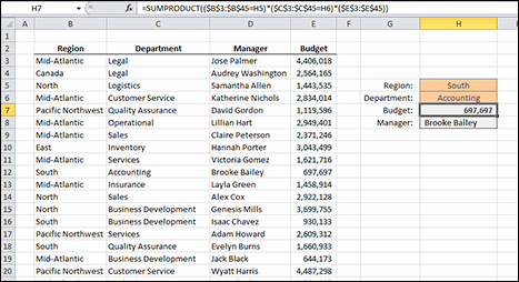
Figure 6-13: A table of departmental budgets.
How it works
SUMPRODUCT compares every cell in a range with a value and returns an array of TRUEs and FALSEs depending on the result. When multiplied with another array, TRUE becomes 1, and FALSE becomes 0. The third parenthetical section in your SUMPRODUCT function does not contain a comparison, because that range contains the value you want to return.
If either the Region comparison or the Department comparison is FALSE, the total for that line will be 0. A FALSE result is converted to 0, and anything times 0 is 0. If both Region and Department match, both comparisons return 1. The two 1s (ones) are multiplied with the corresponding row in column E, and that’s the value returned.
In the example shown in Figure 6-13, when SUMPRODUCT gets to row 12, it multiplies 1 * 1 * 697,697. That number is summed with the other rows, all of which are 0 because they contain at least one FALSE. The resulting SUM is the value 697,697.
Alternative: Returning text with SUMPRODUCT
SUMPRODUCT works this way only when you want to return a number. If you want to return text, all the text values would be treated as 0, and SUMPRODUCT would always return 0.
However, you can pair SUMPRODUCT with the INDEX and ROW functions to return text. If you want to return the manager’s name, for example, you could use this formula:
=INDEX(D:D,SUMPRODUCT(($B$3:$B$45=H5)*($C$3:$C$45=H6)*(ROW($E$3:$E$45))),1)
Instead of including the values from column E, the ROW function is used to include the row numbers in the array. SUMPRODUCT now computes 1 * 1 * 12 when it gets to row 12. The 12 is then used for the row argument in INDEX against the entire column D:D. Because the ROW function returns the row in the worksheet and not the row in your table, INDEX uses the whole column as its range.
Formula 63: Finding the Last Value in a Column
Figure 6-14 shows an unsorted list of invoices. You want to find the last invoice in the list. A simple way to find the last item in the column is to use the INDEX function and count the items in the list to determine the last row.
=INDEX(B:B,COUNTA(B:B)+1)
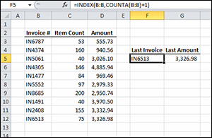
Figure 6-14: A list of invoices.
How it works
The INDEX function when used on a single column needs only a row argument. The third argument indicating the column isn’t necessary. COUNTA is used to count the non-blank cells in column B. That count is increased by 1 because you have a blank cell in the first row. The INDEX function returns the 12th row of column B.
COUNTA counts numbers, text, dates, and anything except blanks. If your data contains blank rows, COUNTA won’t return the desired result.
Alternative: Finding the last number using LOOKUP
INDEX and COUNTA are great for finding values when the range doesn’t contain any blank cells. If you have blanks and the values you’re searching for are numbers, you can use LOOKUP and a really large number. The formula in cell G5 of Figure 6-14 uses this technique.
=LOOKUP(9.99E+307,D:D)
The lookup value is the largest number Excel can handle (just under 1 with 308 zeroes behind it). Because LOOKUP won’t find a value that large, it stops at the last value it does find, and that’s the value returned.
A number like 9.99E+307 is written in exponential notation. The number before the E has one number to the left of the decimal and two to the right. The number after the E is how many places to move the decimal point to show the number in regular notation (307 in this case). A positive number means to move the decimal to the right, and a negative number means to move it left. A number like 4.32E-02 is equivalent to 0.0432.
This LOOKUP method has the additional advantage of returning the last number even if the range has text, blanks, or errors.
Formula 64: Look Up the Nth Instance of a Criterion
One of the limitations of VLOOKUP and other lookup functions is that they find only the first occurrence of a matching value in a list. To find the second, third, or subsequent occurrence, you have to use an array formula.
Figure 6-15 shows a list of salespeople and sale amounts. Next to this list is a filtered list showing sales for only one salesperson. To create this list with formulas, you can’t just use a VLOOKUP, because that will find only the first occurrence. You need to find all the occurrences and list them individually.
The following formula uses a number of functions, including INDEX, SMALL, and ROW. The SMALL function finds the nth smallest row that matches the name, and that row is used in INDEX to return the amount on that row.
=IF(LEN(E3)>0,INDEX ($C$1:$C$26,SMALL(IF(($B$3:$B$26=E3),ROW($B$3:$B$26),""),ROW()-2),1),"")
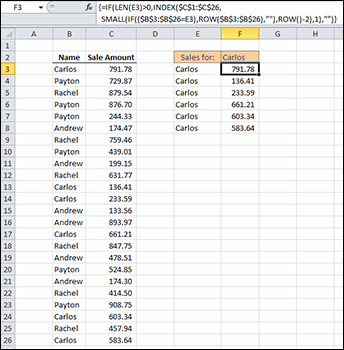
Figure 6-15: A list of sales.
The formula in column E is a bit simpler. It lists the salesperson’s name a number of times equal to the times the name appears in the main list. It uses COUNTIF to determine how many times the name appears.
=IF(COUNTIF($B$3:$B$26,$F$2)>ROW()-3,$F$2,"")
Both the formulas in column E and column D are copied down a sufficient number of times to show all the occurrences.
How it works
The formula in column E repeats the name in F2 if the count of that name is greater than ROW()-3. For cell E3, ROW()-3 returns 0, and “Carlos” is in the main list more than zero times, so the name is shown. In cell E9, however, ROW()-3 returns 6. Carlos’s name appears only six times, so the count of his name is not greater than ROW()-3. In that case, an empty string (two double quotes) is returned.
The formula in column D is an array formula, and you enter it by holding down Ctrl+Shift and then pressing Enter. The formula starts by checking to see whether there is a name in column E. If there isn’t, an empty string is returned. If there is a name, an INDEX function is used to return the value of the nth instance of the name.
The row argument to INDEX uses the SMALL function. SMALL accepts an array (an array of rows and empty strings in this case) for its first argument and a number indicating the nth smallest value. A 2 in the second argument, for example, would find the second smallest number. For the second argument, you use ROW()-2. Because the data starts in row 3, the formula in row 3 returns the first smallest number, the formula in row 4 returns the second smallest number, and so on.
The SMALL function ignores strings and deals only with numbers. You use an IF statement to return the row number when B3:B26 matches the name. If it doesn’t match, an empty string is returned, which SMALL simply ignores. When IF is evaluated for Carlos, the array sent to SMALL looks like this:
{3;"";"";"";"";"";"";"";"";"";13;14;"";"";17;"";"";"";"";"";"";24;"";26}
That’s an array with 24 elements. When Carlos is matched, the row is returned, and SMALL will find the nth smallest row. For the formula in cell F5, SMALL returns 14 (the third smallest number in the array) and INDEX returns the value in row 14 (233.59).
Formula 65: Performing a Case-Sensitive Lookup
VLOOKUP and the other lookup functions don’t care about capitalization when matching values. Using VLOOKUP to match "Bob" and "bob" will return the same result. When case matters, you use Excel’s EXACT function.
Figure 6-16 shows a list of computer ID numbers and the last date someone logged in to that computer. The IDs in row 4 and row 11 are identical except for the case of the two letters in the middle. You want to perform a case-sensitive lookup of the computer ID.
Figure 6-16 also shows the results of two formulas. One uses VLOOKUP, and the other uses EXACT. Although you’ve selected the computer ID from row 11 in cell F4, VLOOKUP returns the result from row 4. The EXACT formula returns the correct result and is shown here:
=INDEX(C1:C12,SUMPRODUCT((EXACT(B3:B12,F4))*(ROW(B3:B12))),1)
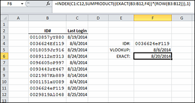
Figure 6-16: A list of computer IDs and login dates.
How it works
By now you’re familiar with using SUMPRODUCT and ROW to feed INDEX with a row number. This formula uses the EXACT function inside SUMPRODUCT. EXACT takes two arguments and returns TRUE if they are exactly the same (including capitalization).
When EXACT is used in SUMPRODUCT or an array formula, you can compare a range of text values to another value and get back an array of TRUEs and FALSEs. In this case, EXACT returns TRUE only when it compares B11 to F4. That TRUE value is converted to a 1 when multiplied by the array of ROW values, and SUMPRODUCT returns 11. All of the other EXACT results are FALSE and return 0.
The result of SUMPRODUCT, 11, is used as the row argument to INDEX, which returns the value from the 11th row in the range C1:C12.
Formula 66: Letting the User Select How to Aggregate Data
Excel’s CHOOSE function is a great way to have different formulas in the same cell and let the user select which formula to use. Figure 6-17 shows a list of sales and three ways to aggregate them. The user can select which aggregator to use by selecting from a drop-down box in cell G7.
=CHOOSE(MATCH(G7,G3:G5,FALSE),SUM(D3:D17),COUNT(D3:D17),AVERAGE(D3:D17))
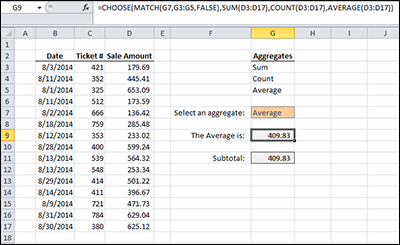
Figure 6-17: Changing the aggregate from the drop-down box in cell G7.
How it works
The CHOOSE function’s first argument is named index_num, and it determines which of the next arguments is returned. It can be a number between 1 and the number of arguments in the function up to 254. The next 254 arguments (only the first one is required) determines what is returned by CHOOSE. If index_num is 1, the second argument is returned; if index_num is 2, the third argument is returned; and so on.
The arguments after index_num are the three ways the user can aggregate the sales data, namely SUM, COUNT, and AVERAGE. The index_num argument is provided by a MATCH function that returns 1, 2, or 3 depending on where the user’s choice (G7) falls in the list of aggregates (G3:G5).
If the user selects Sum, MATCH returns 1 and second argument (SUM) is returned. If the user selects Count, MATCH returns 2, and the third argument (COUNT) is returned. In Figure 6-17, the user selected Average, MATCH returned 3, and the fourth argument (AVERAGE) is returned.
Alternative
Another way to use CHOOSE and MATCH is in combination with the SUBTOTAL function. SUBTOTAL has a number of built-in aggregates that can be applied to a range. For example, if the first argument of SUBTOTAL is 9, the range is summed; if the first argument is 2, the range is counted; and if the first argument is 1, the range is averaged.
=SUBTOTAL(CHOOSE(MATCH(G7,G3:G5,FALSE),9,2,1),D3:D17)
Inside the SUBTOTAL, you can use CHOOSE and MATCH to return the SUBTOTAL aggregate to use. This is more restrictive than simply putting the formula in the CHOOSE function’s arguments because you’re limited to the aggregates allowed by SUBTOTAL.