Chapter 5: Performing Conditional Analysis
Excel provides several worksheet functions for performing conditional analysis, and in this chapter, we show you how to use some of those functions. Conditional analysis means performing different actions depending on whether a condition is met.
 You can download the files for all the formulas at www.wiley.com/go/101excelformula.
Formula 44: Check to See Whether a Simple Condition Is Met
A condition is a value or expression that returns TRUE or FALSE. Based on the value of the condition, a formula can branch into two separate calculations. That is, when the condition returns TRUE, one value or expression is evaluated while the other is ignored. A FALSE condition reverses the flow of the formula, and the first value or expression is ignored and the other evaluated.
Figure 5-1 displays a list of states and six monthly gas prices. For each price, say that you want to determine whether that state’s price in that month is above or below average for all the states for the same month. For higher-than-average prices, you report “High,” and for lower than average, “Low”. A grid below the data is used to report the results.
=IF(C3>AVERAGE(C$3:C$11),”High”,”Low”)
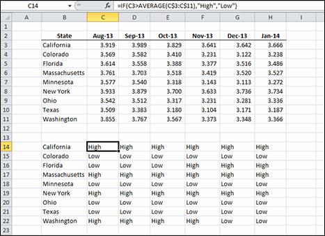
Figure 5-1: Monthly gas prices by state.
How it works
The IF function is the most basic conditional analysis function in Excel. It has three arguments: the condition; what to do if the condition is true; and what to do if the condition is false.
The condition argument in this example is C3>AVERAGE(C$3:C$11). Condition arguments must be structured to return TRUE or FALSE, and that usually means that there is a comparison operation (like an equal sign or greater-than sign) or another worksheet function that returns TRUE or FALSE (such as ISERR or ISBLANK). In this example, the condition has a greater-than sign and compares the value in C3 to the average of all the values in C3:C11.
 In this formula, the reference to C3 is relative to both columns and rows and will change as the formula is copied to different cells. The C$3:C$11 reference is relative to columns but absolute to rows. This reference will change as it is copied to different columns, but not to different rows.
 See Chapter 1 for more information on absolute and relative cell references.
If the condition argument returns TRUE, the second argument of the IF function is returned to the cell. The second argument is “High” and because the value in C3 is indeed larger than the average, cell C14 shows the word “High”.
Cell C15 compares the value in C4 to the average. Because it is lower, the condition argument returns FALSE and the third argument is returned. Cell C15 shows “Low”, the third argument of the IF function.
Formula 45: Checking for Multiple Conditions
Simple conditions like the one shown in Formula 44 can be strung together. This is known as nesting functions. The value_if_true and value_if_false arguments can contain simple conditions of their own. This allows you test more than one condition where subsequent conditions are dependent on the first one.
Figure 5-2 shows a spreadsheet with two user input fields for the type of automobile and a property of that automobile type. The properties are listed in two ranges below the user input fields. For this example, when the user selects the type and property, you want a formula to report whether the user has identified a coupe, a sedan, a pickup, or an SUV, as follows:
=IF(E2="Car",IF(E3="2-door","Coupe","Sedan"),IF(E3="Has Bed","Pickup","SUV"))
How it works
With some conditional analysis, the result of the first condition causes the second condition to change. In this case, if the first condition is Car, the second condition is 2-door or 4-door. But if the first condition is Truck, the second condition changes to either Has Bed or No Bed. The data validation in cell E3 in Figure 5-2 changes to allow only the appropriate choices based on the first condition. See the “Conditional data validation” sidebar in this chapter for instructions on how to create the data validation in cell E3.
As mentioned previously, Excel provides the IF function to perform conditional analyses. You can also nest IF functions — that is, use another IF function as an argument to the first IF function — when you need to check more than one condition. In this example, the first IF checks the value of E2. Rather than return a value if TRUE, the second argument is another IF formula that checks the value of cell E3. Similarly, the third argument doesn’t simply return a value of FALSE, but contains a third IF function that also evaluates cell E3.
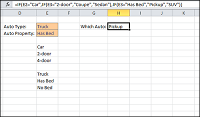
Figure 5-2: A model for selecting an automobile.
In Figure 5-2, the user has selected “Truck”. The first IF returns FALSE because E2 doesn’t equal “Car” and the FALSE argument is evaluated. In that argument, E3 is seen to be equal to “Has Bed” and the TRUE condition (“Pickup”) is returned. If the user had selected “No Bed”, the FALSE condition (“SUV”) would have been the result.
In Excel versions prior to 2007, you can only nest functions up to seven levels deep. Starting in Excel 2007, that limit was increased to 64 levels. As you can imagine, even seven levels can be hard to read and maintain. If you need more than three or four levels, it’s good idea to investigate other methods.
 Conditional data validation
The user input fields in Figure 5-2 are actually data validation lists. The user can make selections from a drop-down box rather than typing in the values. The Data Validation in cell E3 uses an interesting technique with an INDIRECT function to change its list depending on the value in E2.
The worksheet contains two named ranges. The range named Car points to E6:E7 and the range named Truck points to E10:E11. The names are identical to choices in the E2 Data Validation list. The following figure shows the Data Validation dialog box for cell E3. The Source is an INDIRECT function with E2 as the argument.
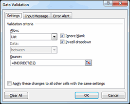
The INDIRECT function takes a text argument that it resolves into a cell reference. In this case, because E2 is “Truck”, the formula becomes =INDIRECT(“Truck”). Because Truck is a named range, INDIRECT returns a reference to E10:E11 and the values in those cells become the choices. If E2 contained “Car”, INDIRECT would return E6:E7 and those values would become the choices.
One problem with this type of conditional data validation is that when the value in E2 is changed, the value in E3 does not change. The choices in E3 change, but the user still has to select from the available choices or your formulas may return inaccurate results.
Alternative 1: Looking up values
When you have too many nested IF functions, your formulas can become long and hard to manage. Figure 5-3 shows a slightly different setup to the auto selecting model. Instead of hardcoding the results in nested IF functions, the results are entered into the cells next to their properties; for example, “Sedan” is entered in the cell next to “4-door”.
The new formula is
=IF(E2="Car",VLOOKUP(E3,E6:F7,2,FALSE),VLOOKUP(E3,E10:F11,2,FALSE))
You can use this formula to return the automobile type. The IF condition is the same, but now a TRUE result looks up the proper value in E6:E7 and a FALSE result looks it up in E10:F11. You can learn more about VLOOKUP in Chapter 6.
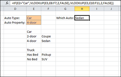
Figure 5-3: A different auto selector model.
Formula 46: Check Whether Condition1 AND Condition2 Are Met
In addition to nesting conditional functions, such functions can be evaluated together inside an AND function. This is useful when two or more conditions need to be evaluated at the same time to determine where the formula should branch.
Figure 5-4 shows a listing of inventory items, their quantities, and the discount that applies when they are sold. The inventory items are structured with three sections divided by hyphens. The first section is the department; the second section determines whether the item is a part, a subassembly, or a final assembly; and the third condition is a unique four-digit number. For this example, you want to assign a discount of 10 percent to only those items that are in department 202 and are final assemblies. All other items have no discount.
=IF(AND(LEFT(B3,3)="202",MID(B3,5,3)="FIN"),0.1,0)
How it works
The IF function returns 10 percent if TRUE and 0 percent if FALSE. For the condition argument (the first argument), you need an expression that returns TRUE if both the first section of the item number is 202 and the second section is FIN. Excel provides the AND function to accomplish this task. The AND function takes up to 255 logical arguments separated by commas. Logical arguments are expressions that return either TRUE or FALSE. For this example, you use only two logical arguments.
The first logical argument, LEFT(B3,3)=“202”, returns TRUE if the first three characters of B3 are equal to 202. The second logical argument, MID(B3,5,3)=“FIN”, returns TRUE if the three digits starting at the fifth position are equal to FIN.
See Chapter 3 for more about text manipulation functions.
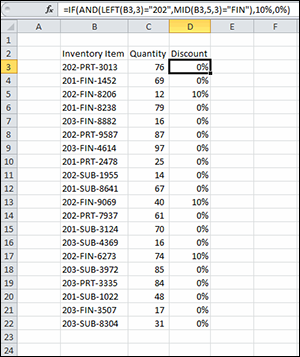
Figure 5-4: An inventory listing.
With the AND function, all logical arguments must return TRUE for the entire function to return TRUE. If even one of the logical arguments returns FALSE, the AND function returns FALSE. Table 5-1 shows the results of the AND function with two logical arguments.
Table 5-1: A Truth Table for the AND Function
|
First Logical Argument |
Second Logical Argument |
Result of AND function |
|
TRUE |
TRUE |
TRUE |
|
TRUE |
FALSE |
FALSE |
|
FALSE |
TRUE |
FALSE |
|
FALSE |
FALSE |
FALSE |
In cell D3, the first logical condition returns TRUE because the first three characters of the item number are “202”. The second logical condition returns FALSE because the middle section of the item number is “PRT”, not “FIN”. According to Table 5-1, a TRUE and a FALSE condition returns FALSE and 0 percent is the result. Cell D5, on the other hand, returns TRUE because both logical conditions return TRUE.
Alternative 1: Referring to logical conditions in cells
The AND function in Figure 5-4 includes two logical conditions that evaluate to TRUE or FALSE. The arguments to AND can also reference cells as long as those cells evaluate to TRUE or FALSE. When building a formula with the AND function, it can be useful to break out the logical conditions into their own cells. In Figure 5-5, the inventory listing is modified to show two extra columns. These columns can be inspected to determine why a particular item does or does not get the discount.
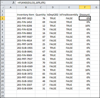
Figure 5-5: A modified inventory listing.
With these modifications, the result doesn’t change, but the formula becomes
=IF(AND(D3,E3),10%,0%)
Formula 47: Check Whether Condition1 OR Condition2 Is Met
In Formula 46, you apply a discount to certain products based on their item number. In this example, you expand the number of products eligible for the discount. As before, only final assembly products get the discount, but the departments will be expanded to include both departments 202 and 203. Figure 5-6 shows the inventory list and the new discount schedule.
=IF(AND(OR(LEFT(B3,3)="202",LEFT(B3,3)="203"),MID(B3,5,3)="FIN"),10%,0%)
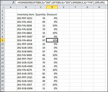
Figure 5-6: A revised discount scheme.
How it works
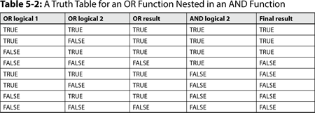
You expand the conditional argument to the IF function to account for the changes in the discount scheme. The AND function is restrictive because all the arguments must be TRUE for AND to return TRUE. Conversely, the OR function is inclusive. With OR, if any one of the arguments is TRUE, the entire function returns TRUE. In this example, you nest an OR function inside the AND function, making it one of the arguments. Table 5-2 shows a truth table for how these nested functions work.
A truth table is a table used in logic that breaks a large Boolean (True or False) result into its Boolean components. Each row of the table is evaluated independently of the other rows. Truth tables are useful in simplifying complex Boolean results and identifying patterns.
Cell D9 in Figure 5-6 shows a previously undiscounted product that receives a discount under the new scheme. The OR section, OR(LEFT(B9,3)=“202”,LEFT(B9,3)=“203”), returns TRUE because one of its arguments returns TRUE.
Formula 48: Sum All Values That Meet a Certain Condition
Simple conditional functions like IF generally work on only one value or cell at a time. Excel provides some different conditional functions for aggregating data, such as summing.
Figure 5-7 shows a listing of accounts with positive and negative values. You want to sum all the negative balances, which you will later compare to the sum of all the positive balances to ensure that they are equal. Excel provides the SUMIF function to sum values based on a condition.
=SUMIF(C3:C12,"<0")
How it works
SUMIF takes each value in C3:C12 and compares it to the condition (the second argument in the function). If the value is less than zero, it meets the condition and is included in the sum. If it is zero or greater, the value is ignored. Text values and blank cells are also ignored. For the example in Figure 5-7, cell C3 is evaluated first. Because it is greater than zero, it is ignored. Next, cell C4 is evaluated. It meets the condition of being less than zero, so it is added to the total. This process continues for each cell. When it's complete, cells C4, C7, C8, C9, and C11 are included in the sum and the others are not.
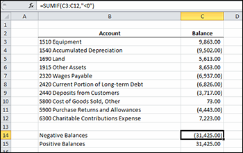
Figure 5-7: Sum values less than zero.
The second argument of SUMIF, the condition to be met, has quotation marks around it. Because this example uses a less-than sign, you have to create a string that represents the expression.
The SUMIF function has an optional third argument called the sum_range. So far, you’ve applied the condition to the very numbers that you’re summing. By using the third argument, you can sum a range of numbers but apply your conditions to a different range. Figure 5-8 shows a listing of regions and their associated sales. To sum the sales for the East region, use the formula =SUMIF(B2:B11,“East”,C2:C11).
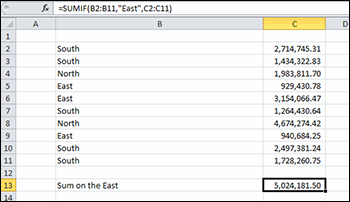
Figure 5-8: List of regions and sales values.
Alternative 1: Summing greater than zero
Figure 5-8, shown previously, also shows the total of all the positive balances. The formula for that calculation is =SUMIF(C3:C12,“>0”). Note that the only difference between this formula and the previous example formula is the expression string. Instead of “<0” as the second argument, this formula has “>0”. See the “Constructing criteria in SUMIF” sidebar in this chapter for more examples of expression strings.
You don't have to include zero in the calculation because you're summing, and zero never changes a sum. If, however, you were interested in summing numbers greater or less than 1,000, you couldn't simply use “<1000” and “>1000” as your second arguments because you would never include anything that was exactly 1,000. When you use a greater-than or less-than nonzero number in a SUMIF, make the greater-than number a greater than or equal to, such as “>=1000”, or make the less-than number a less than or equal to, such as “<=1000”. Don't use the equal sign for both, just one. This approach ensures that you include any numbers that are exactly 1,000 in one or the other calculation, but not both.
Formula 49: Sum All Values That Meet Two or More Conditions
The limitation of SUMIF shown in Formula 48 is that it works with only one condition. In Excel 2010 and later versions, you can use the SUMIFS function when more than one condition is needed.
Figure 5-9 shows a partial listing of countries and their gross domestic product (GDP) from 2000 to 2009. You want to total Brazil's GDP from 2003 to 2006. You use the Excel SUMIFS worksheet function to sum values when two or more conditions must be met, such as Country and Year in this example.
=SUMIFS(D3:D212,B3:B212,G3,C3:C212,">="&G4,C3:C212,"<="&G5)
How it works
SUMIFS arguments start with the range that contains the value you want to sum. The remaining arguments are in pairs that follow the pattern criteria_range, criteria. Because of the way the arguments are laid out, SUMIFS will always have an odd number of arguments. The first criteria pair is required; without at least one condition, SUMIFS would be no different than SUM. The remaining pairs of conditions, up to 126 of them, are optional.
In this example, each cell in D3:D212 is added to the total only if the corresponding values in B3:B212 and C3:C212 meet their respective conditions. The condition for B3:B212 is that it matches whatever is in cell G3. There are two year conditions because you need to define the first year and last year of your year range. The first year is in cell G4 and the last year is in cell G5. Those two cells are concatenated with greater-than-or-equal-to and less-than-or-equal-to, respectively, to create the year conditions. Only if all three conditions are true is the value included in the total.
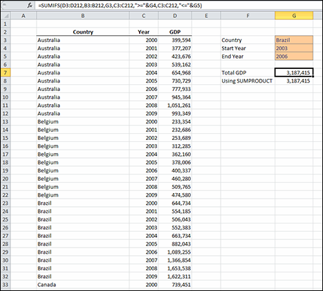
Figure 5-9: Calculating the gross domestic product of a selected country between two years.
Alternative: SUMPRODUCT
The SUMIFS function was introduced in Excel 2010. Prior to that version of Excel, the best way to sum values with two or more conditions was to use SUMPRODUCT. For this application, the SUMPRODUCT function needs only one argument, but it's a big one. The SUMPRODUCT equivalent of this section’s example is =SUMPRODUCT((B3:B212=G3)*(C3:C212>=G4)*(C3:C212<=G5)*(D3:D212)). This formula uses a pairing of ranges and conditions similar to the pairing of arguments in SUMIFS. Each set of parentheses (except the last one) contains a range, a comparison operator, and a comparison value. The last set of parentheses simply contains the range to sum. Excel evaluates each set of parentheses as an array. See the “SUMPRODUCT and arrays” sidebar in this chapter to learn how Excel combines arrays using SUMPRODUCT. Unlike SUMIFS, the parentheses aren't required to be in any order. The range to sum could be the first set or somewhere in the middle and the result would be the same.
Formula 50: Sum Values That Fall between a Given Date Range
One way that you can use SUMIF with two or more conditions is to add or subtract multiple SUMIF calculations. If the two conditions operate on the same range, this is an effective way to use multiple conditions. When you want to test different ranges, the formulas get tricky because you have to make sure that you don’t double count values.
Figure 5-10 shows a list of dates and amounts. You want to find the sum of the values that are between June 23 and June 29, inclusive. The starting and ending dates will be put in cells F4 and F5, respectively.
=SUMIF(B3:B20,"<="&F5,C3:C20)-SUMIF(B3:B20,"<"&F4,C3:C20)
How it works
This technique subtracts one SUMIF from another to get the desired result. The first SUMIF, SUMIF(B3:B20,"<="&F5,C3:C20), returns the sum of the values that are less than or equal to the date in F5, which is June 29 in this example. The conditional argument is the less-than-or-equal-to operator concatenated to the cell reference F5. If that was the whole formula, the result would be 5,962.33. However, you want only values that are also greater than or equal to June 23. You therefore want to exclude values that are less than June 23. The second SUMIF achieves that goal. Sum everything less than or equal to the later date and subtract everything less than the earlier date to get the sum of values between the two dates.
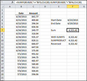
Figure 5-10: Summing values that are between two dates.
Alternative 1: SUMIFS
If you're using Excel version 2010 or greater, you can use the SUMIFS function to achieve the same result as the preceding formula. You may even find SUMIFS to be more intuitive than the subtraction technique. The formula =SUMIFS(C3:C20,B3:B20,"<="&F5,B3:B20,">="&F4) sums the values in C3:C20 that correspond to the values in B3:B20 that meet the criteria pairs. The first criteria pair is identical to the first SUMIF criteria, "<="&F5. The second criteria pair limits the dates to greater than or equal to the start date.
Alternative 2: SUMPRODUCT
You can use the SUMPRODUCT function in place of SUMIF. The formula =SUMPRODUCT((B3:B20<=F5)*(B3:B20>=F4)*(C3:C20)) returns the same result as SUMIF. See Formula 49 for a detailed explanation of how SUMPRODUCT uses arrays.
Formula 51: Get a Count of Values That Meet a Certain Condition
Summing values isn’t the only aggregation you can do in Excel. As with SUMIF and SUMIFS, Excel provides functions for conditionally counting values in a range.
Figure 5-11 shows a partial listing of countries and their gross domestic product (GDP) from 2000 to 2009. For this example, you want to know how many times the GDP was greater than or equal to 1 million. The criteria to be applied will be in cell G3.
=COUNTIF(D3:D212,G3)
How it works
The COUNTIF function works very similarly to the SUMIF function from Formula 48. The obvious difference, as the name suggests, is that it counts entries that meet the criteria rather than sums them. Another difference is that the formula uses no optional third argument as the SUMIF formula does. With SUMIF, you can sum a range that's different from the range to which the criterion is applied. With COUNTIF, however, doing that wouldn't make sense because counting a different range would get the same result.
The formula in this example uses a slightly different technique to construct the criteria argument. The string concatenation occurs all in cell G3 rather than in the function's second argument. If you had used the same approach as SUMIF in Formula 48, the second argument would look like ">=1000000" or ">="&G3 rather than just pointing to G3. You may also note that the formula in G3, =">="&10^6, uses the exponent operator, or caret (^), to calculate 1 million. Representing large numbers using the caret can help reduce errors caused by miscounting the number of zeros that you typed.
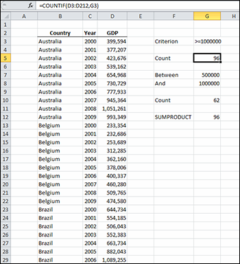
Figure 5-11: Count the number of country and year combinations whose gross domestic product meets a specified criterion.
Alternative: SUMPRODUCT
You can also use SUMPRODUCT to count conditionally. Formula 49 discusses how you can use SUMPRODUCT in place of SUMIFS to sum conditionally. It's the same for COUNTIF, with a few minor changes. The formula =SUMPRODUCT(--(D3:D212>10^6)) returns 96 just as COUNTIF did.
You may have noticed that double negative in the function's argument. In Formula 49, we discussed how multiplying TRUE makes it act like a 1 and multiplying FALSE makes it act like zero. This example, however, uses only one condition, D3:D212>10^6, so you have nothing to multiply, and the TRUEs and FALSEs never get converted to 1s and 0s. The double negative performs a mathematical operation on the array, forcing the conversion, but since it's doubled up, it doesn't have any effect on the result. The TRUEs are converted to -1 with the first negation and converted back to 1 with the second. The FALSEs are converted to zero simply because some math is being done, but negation has no effect on zero so it stays the same throughout.
Formula 52: Get a Count of Values That Meet Two or More Conditions
The SUMIF function has its COUNTIF cousin. Of course, Microsoft couldn’t introduce SUMIFS for summing multiple conditions without also introducing COUNTIFS to count them. Microsoft did just that in Excel 2010.
Figure 5-12 contains a list of Alpine Skiing medalists from the 1972 Winter Olympics. For this example, you would like to know how many silver medalists have an ö in their name. The letter you're looking for is typed in cell I3, and the type of medal is in cell I4. (See the “Finding the code for a nonstandard character” sidebar for how to obtain the ö character and other nonstandard characters.)
=COUNTIFS(C3:C20,"*"&I3&"*",F3:F20,I4)
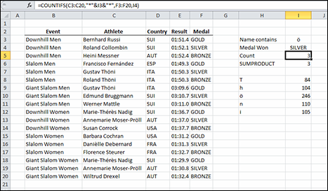
Figure 5-12: The letter ö shows up the names of the1972 alpine skiing Olympic silver medalists three times.
How it works
The criteria_range and criteria arguments come in pairs, just as in SUMIFS. Whereas SUMIFS will always have an odd number of arguments, COUNTIFS will always have an equal number.
The first criteria_range argument is the list of athlete's names in C3:C20. The matching criteria argument, "*" & I3 & "*", surrounds whatever is in I3 with asterisks. Asterisks are wildcard characters in COUNTIFS that stand for zero, one, or more characters of any kind. By including an asterisk both before and after the character, you ask Excel to count all the names that include that character anywhere within the name. That is, you don't care whether there are zero, one, or more characters before ö and you don't care whether there are zero, one, or more characters after ö — as long as that character is in there somewhere.
The second criteria_range, criteria argument pair counts those entries in F3:F20 that are SILVER (the value typed into I4). Only those rows in which both the first argument pair and second argument pair match (only rows in which the athlete's name contains ö and the medal won was silver) are counted. In this example, Gustav Thöni won the silver in the Men's Slalom and Annemarie Moser-Pröll placed in both the Women's Downhill and the Women's Giant Slalom, for a count of three.
Alternative: SUMPRODUCT
The COUNTIFS worksheet function was introduced in Excel 2010. If you're using an earlier version, you can use SUMPRODUCT to get the same result. The formula =SUMPRODUCT((NOT(ISERR(FIND(I3,C3:C20))))*(F3:F20=I4)) will also return the proper count, although it's a little tougher to read. In Formula 49, you see how SUMPRODUCT multiplies arrays of TRUEs and FALSEs to sum based on conditions. For the example in this section, SUMPRODUCT does the same thing. Everything to the left of the asterisk will turn into an array of 18 TRUEs and FALSEs, and everything to the right will do the same. When a TRUE is used in a mathematical operation, it acts like the number one and FALSE acts like zero. Whenever a FALSE is in either the first or second array, the result will be zero. If both the first and second array contain 1, the formula multiplies 1 * 1 to get a 1 in the final array. The result of multiplying those two arrays together is an 18-element array of 1s and 0s. When SUMPRODUCT adds up the 1s, it effectively counts the rows where both conditions are met.
The second array, F3:F20=I4, is pretty straightforward. Each cell in F3:F20 is compared to I4 and a TRUE or a FALSE is included in that array. The first array is a little more complicated than the first. You know that the result needs to be a bunch of TRUEs and FALSEs, so you need to come up with an expression that returns TRUE or FALSE. The FIND function returns the position of a string in another string. For example, FIND("ö","Thöni") returns 3 because "ö" is the third letter in the name "Thöni". If FIND can't find the letter, it returns an error.
The ISERR function returns either TRUE or FALSE depending on whether the expression is any error except #N/A!. Using ISERR gets you close to your goal because it returns TRUE or FALSE. The problem is that it returns the wrong one. It returns TRUE if FIND can't find ö in the name, but you want it to return TRUE when it does find it. The NOT function comes to the rescue. The NOT function takes a TRUE or a FALSE and turns into the other one. If ö is in the name, FIND returns a number (like the number 10 when it looks at Roland Thöni). Then, ISERR(10) returns FALSE because 10 isn't an error, it's a number. Finally, NOT(FALSE) returns TRUE.
Formula 53: Get the Average of All Numbers That Meet a Certain Condition
After summing and counting, taking an average of a range of numbers is the next most common aggregator. The average, also known as the arithmetic mean, is the sum of the numbers divided by the count of the numbers.
As in the example for Formula 52, Figure 5-13 shows medalists’ results from the 1972 Winter Olympics. For this example, you want to determine the average result, but only for skiers from Switzerland. The country code is entered in cell I3 so that it can be easily changed to a different country.
=AVERAGEIF(D3:D20,I3,E3:E20)
How it works
Excel provides the AVERAGEIF function to accomplish just what you want. Like its cousin the SUMIF function, AVERAGEIF has a criteria_range and a criteria argument. The final argument is the range to average. In this example, each cell in E3:E20 is either included in or excluded from the average, depending on whether the corresponding cell in D3:D20 meets the criteria.
If no rows meet the criteria in AVERAGEIF, the function returns the #DIV/0! error.
Alternative
The AVERAGEIF function simply adds up the average_range for all rows that meet the criteria and then divides by the number of rows. This same result can be had by using the SUMIF function divided by the COUNTIF function. Using the list from Figure 5-13, the formula =SUMIF(D3:D20,I3,E3:E20)/COUNTIF(D3:D20,I3) can also be used to find the conditional average.
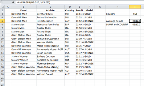
Figure 5-13: Averaging results based on a country.
Formula 54: Get the Average of All Numbers That Meet Two or More Conditions
In Excel 2010, Microsoft introduced AVERAGEIFS along with SUMIFS and COUNTIFS to allow you to average a range of numbers based on more than one condition.
Continuing the analysis of skiing times as an example (see Formulas 52 and 53), Figure 5-14 shows some results of the 1972 Winter Olympics. In this case, you want to determine the average time based on more than one condition. The country, gender, and medal are entered into cell I3:I5. You want to average only those results that meet all three criteria:
=AVERAGEIFS(E3:E20,D3:D20,I3,B3:B20,"*"&I4,F3:F20,I5)
How it works
The AVERAGEIFS function is structured very similarly to the SUMIFS function. The first argument is the range to average and is followed by up to 127 pairs of criteria_range/criteria arguments. The three criteria pairs are
- D3:D20,I3, which includes only those rows where the country code is SUI
- B3:B20,"*"&I4, which includes only those rows where the event name ends with the word “Women”
- F3:F20,I5, which includes only those rows where the medal is GOLD
When all three conditions are met, the time in the Result column is averaged.
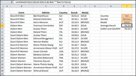
Figure 5-14: Averaging on three conditions.
Alternative
You can replace the AVERAGEIFS function with SUMIFS and COUNTIFS. Doing so is useful if you’re using a version of Excel prior to 2010, when AVERAGEIFS was introduced. The formula =SUMIFS(E3:E20,D3:D20,I3,B3:B20,"*"&I4,F3:F20,I5)/COUNTIFS(D3:D20,I3,B3:B20,"*"&I4,F3:F20,I5) returns the same result as AVERAGEIFS. Notice how similar the arguments in SUMIFS and COUNTIFS are to those in AVERAGIFS. If it’s available, AVERAGEIFS is the preferred method because any changes to the criteria have to be made in only one place.