Chapter 9: Using Formulas with Conditional Formatting

Conditional Formatting is the term given to the functionality with which Excel dynamically changes the formatting of a value, cell, or range of cells based on a set of conditions you define. Conditional formatting allows you to look at your Excel reports and make split-second determinations on which values are “good” and which are “bad,” all based on formatting.

In this chapter, you explore a few examples of how you can use the Conditional Formatting feature in Excel in conjunction with formulas to add an extra layer of visualizations to your analyses.

The Conditional Formatting feature is fairly robust and includes many bells and whistles that we don’t cover here. To adhere to the spirit of this book, we focus on the techniques for applying conditional formatting with formulas.

You can download the files for all the formulas at www.wiley.com/go/101excelformula.

Formula 93: Highlight Cells That Meet Certain Criteria

One of the more basic Conditional Formatting rules that you can create is the highlighting of cells that meet some business criteria. This first example demonstrates the formatting of cells that fall under a hard-coded value of 4000 (see Figure 9-1).

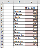
Figure 9-1: The cells in this table are conditionally formatted to show as shaded for values under 4000.

How it works

To build this basic formatting rule, follow these steps:

1. Select the data cells in your target range (cells C3:C14 in this example), click the Home tab of the Excel Ribbon, and then select Conditional Formatting⇒New Rule. The New Formatting Rule dialog box opens, as shown in Figure 9-2.
2. In the list box at the top of the dialog box, click the Use a Formula to Determine which Cells to Format option. This selection evaluates values based on a formula you specify. If a particular value evaluates to TRUE, the conditional formatting is applied to that cell.
3. In the formula input box, enter the formula shown here. Note that you are simply referencing the first cell in the target range. You don’t need to reference the entire range.

   =C3<4000

   Note that in the formula, you exclude the absolute reference dollar symbols ($) for the target cell (C3). If you click cell C3 instead of typing the cell reference, Excel will automatically make your cell reference absolute. It’s important that you don’t include the absolute reference dollar symbols in your target cell because you need Excel to apply this formatting rule based on each cell’s own value.

4. Click the Format button. This opens the Format Cells dialog box, where you have a full set of options for formatting the font, border, and fill for your target cell. After you have completed choosing your formatting options, click the OK button to confirm your changes and return to the New Formatting Rule dialog box.
5. Back in the New Formatting Rule dialog box, click the OK button to confirm your formatting rule.

   

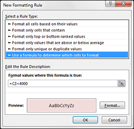
   Figure 9-2: Configure the New Formatting Rule dialog box to apply the needed formula rule.

   If you need to edit your conditional formatting rule, simply place your cursor in any of the data cells within your formatted range and then go to the Home tab and select Conditional Formatting⇒Manage Rules, which opens the Conditional Formatting Rules Manager dialog box. Click the rule you want to edit and then click the Edit Rule button.

Formula 94: Highlight Cells Based on the Value of Another Cell

In many cases, you will base the formatting rule for your cells on how they compare to the value of another cell. Take the example illustrated in Figure 9-3. Here, the cells are conditionally highlighted if their respective values fall below the Prior Year Average shown in cell B3.

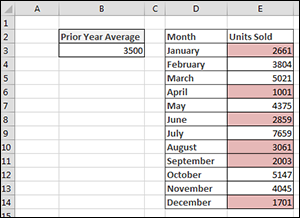
Figure 9-3: The cells in this table are conditionally formatted to show red for values falling below the Prior Year Average.

How it works

To build this basic formatting rule, follow these steps:

1. Select the data cells in your target range (cells E3:C14 in this example), click the Home tab of the Excel Ribbon, and then select Conditional Formatting⇒New Rule. This opens the New Formatting Rule dialog box shown in Figure 9-4.
2. In the list box at the top of the dialog box, click the Use a Formula to Determine which Cells to Format option. This selection evaluates values based on a formula you specify. If a particular value evaluates to TRUE, the conditional formatting is applied to that cell.
3. In the formula input box, enter the formula shown with this step. Note that you are simply comparing your target cell (E3) with the value in the comparison cell ($B$3). As with standard formulas, you need to ensure that you use absolute references so that each value in your range is compared to the appropriate comparison cell.

   =E3<$B$3

   Note that in the formula, you exclude the absolute reference dollar symbols ($) for the target cell (E3). If you click cell E3 instead of typing the cell reference, Excel automatically makes your cell reference absolute. It’s important that you don’t include the absolute reference dollar symbols in your target cell because you need Excel to apply this formatting rule based on each cell’s own value.

4. Click the Format button. This opens the Format Cells dialog box, where you have a full set of options for formatting the font, border, and fill for your target cell. After you have completed choosing your formatting options, click the OK button to confirm your changes and return to the New Formatting Rule dialog box.
5. Back in the New Formatting Rule dialog box, click the OK button to confirm your formatting rule.

   

   Figure 9-4: Configure the New Formatting Rule dialog box to apply the needed formula rule.

   If you need to edit your conditional formatting rule, simply place your cursor in any of the data cells within your formatted range and then go to the Home tab and select Conditional Formatting⇒Manage Rules. This opens the Conditional Formatting Rules Manager dialog box. Click the rule you want to edit and then click the Edit Rule button.

Formula 95: Highlight Values That Exist in List1 but not List2

You may often be asked to compare two lists and pick out the values that are in one list but not the other. Conditional formatting is an ideal way to present your findings. Figure 9-5 illustrates a conditional formatting exercise that compares customers from 2013 and 2014, highlighting those customers in 2014 who are new customers (they were not customers in 2013).

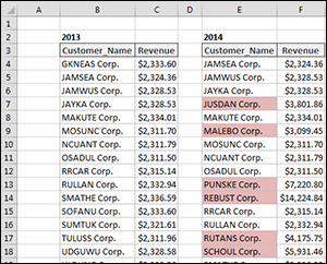
Figure 9-5: You can conditionally format the values that exist in one list but not the other.

How it works

To build this basic formatting rule, follow these steps:

1. Select the data cells in your target range (cells E4:E28 in this example), click the Home tab of the Excel Ribbon, and then select Conditional Formatting⇒New Rule. This opens the New Formatting Rule dialog box shown in Figure 9-6.
2. In the list box at the top of the dialog box, click the Use a Formula to Determine which Cells to Format option. This selection evaluates values based on a formula you specify. If a particular value evaluates to TRUE, the conditional formatting is applied to that cell.
3. In the formula input box, enter the formula shown with this step. Note that you use the COUNTIF function to evaluate whether the value in the target cell (E4) is found in your comparison range ($B$4:$B$21). If the value is not found, the COUNTIF function will return a 0, thus triggering the conditional formatting. As with standard formulas, you need to ensure that you use absolute references so that each value in your range is compared to the appropriate comparison cell.

   =COUNTIF($B$4:$B$21,E4)=0

   Note that in the formula, you exclude the absolute reference dollar symbols ($) for the target cell (E4). If you click cell E4 instead of typing the cell reference, Excel automatically makes your cell reference absolute. It’s important that you don’t include the absolute reference dollar symbols in your target cell because you need Excel to apply this formatting rule based on each cell’s own value.

   For more details on the COUNTIF function, see Formula 51: Get a Count of Values That Meet a Certain Condition, in Chapter 5.

4. Click the Format button. This opens the Format Cells dialog box, where you have a full set of options for formatting the font, border, and fill for your target cell. After you have completed choosing your formatting options, click the OK button to confirm your changes and return to the New Formatting Rule dialog box.
5. In the New Formatting Rule dialog box, click the OK button to confirm your formatting rule.

   

   Figure 9-6: Configure the New Formatting Rule dialog box to apply the needed formula rule.

   If you need to edit your conditional formatting rule, simply place your cursor in any of the data cells within your formatted range and then go to the Home tab and select Conditional Formatting⇒Manage Rules. This opens the Conditional Formatting Rules Manager dialog box. Click the rule you want to edit and then click the Edit Rule button.

Formula 96: Highlight Values That Exist in List1 and List2

You may often need to compare two lists and pick out only the values that exist in both lists. Conditional formatting is an ideal way to accomplish this task. Figure 9-7 illustrates a conditional formatting exercise that compares customers from 2013 and 2014, highlighting those customers in 2014 who are in both lists.

Figure 9-7: You can conditionally format the values that exist in both lists.

How it works

To build this basic formatting rule, follow these steps:

1. Select the data cells in your target range (cells E4:E28 in this example), click the Home tab of the Excel Ribbon, and select Conditional Formatting⇒New Rule. This opens the New Formatting Rule dialog box shown in Figure 9-8.
2. In the list box at the top of the dialog box, click the Use a Formula to Determine which Cells to Format option. This selection evaluates values based on a formula you specify. If a particular value evaluates to TRUE, the conditional formatting is applied to that cell.
3. In the formula input box, enter the formula shown with this step. Note that you use the COUNTIF function to evaluate whether the value in the target cell (E4) is found in your comparison range ($B$4:$B$21). If the value is found, the COUNTIF function returns a number greater than 0, thus triggering the conditional formatting. As with standard formulas, you need to ensure that you use absolute references so that each value in your range is compared to the appropriate comparison cell.

   =COUNTIF($B$4:$B$21,E4)>0

   Note that in the formula, you exclude the absolute reference dollar symbols ($) for the target cell (E4). If you click cell E4 instead of typing the cell reference, Excel automatically makes your cell reference absolute. It’s important that you don’t include the absolute reference dollar symbols in your target cell because you need Excel to apply this formatting rule based on each cell’s own value.

   For more detail on the COUNTIF function, see Formula 51: Get a Count of Values That Meet a Certain Condition, in Chapter 5.

4. Click the Format button. This opens the Format Cells dialog box, where you have a full set of options for formatting the font, border, and fill for your target cell. After you have completed choosing your formatting options, click the OK button to confirm your changes and return to the New Formatting dialog Rule box.
5. Back in the New Formatting Rule dialog box, click the OK button to confirm your formatting rule.

   

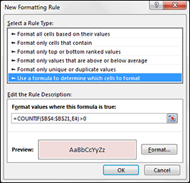
   Figure 9-8: Configure the New Formatting Rule dialog box to apply the needed formula rule.

   If you need to edit your conditional formatting rule, simply place your cursor in any of the data cells within your formatted range and then go to the Home tab and select Conditional Formatting⇒Manage Rules. This opens the Conditional Formatting Rules Manager dialog box. Click the rule you want to edit and then click the Edit Rule button.

Formula 97: Highlight Weekend Dates

When working with timecards and scheduling, you often benefit from being able to easily pinpoint any dates that fall on the weekends. The conditional formatting rule illustrated in Figure 9-9 highlights all the weekend dates in the list of values.

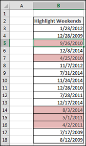
Figure 9-9: You can conditionally format any weekend dates in a list of dates.

How it works

To build this basic formatting rule, follow these steps:

1. Select the data cells in your target range (cells B3:B18 in this example), click the Home tab of the Excel Ribbon, and then select Conditional Formatting⇒New Rule. This opens the New Formatting Rule dialog box shown in Figure 9-10.
2. In the list box at the top of the dialog box, click the Use a Formula to Determine which Cells to Format option. This selection evaluates values based on a formula you specify. If a particular value evaluates to TRUE, the conditional formatting is applied to that cell.
3. In the formula input box, enter the formula shown with this step. Note that you use the WEEKDAY function to evaluate the weekday number of the target cell (B3). If the target cell returns as weekday 1 or 7, it means the date in B3 is a weekend date. In this case, the conditional formatting will be applied.

   =OR(WEEKDAY(B3)=1,WEEKDAY(B3)=7)

   Note that in the formula, you exclude the absolute reference dollar symbols ($) for the target cell (B3). If you click cell B3 instead of typing the cell reference, Excel will automatically make your cell reference absolute. It’s important that you don’t include the absolute reference dollar symbols in your target cell because you need Excel to apply this formatting rule based on each cell’s own value.

   For more detail on the WEEKDAY function, see Formula 29: Extracting Parts of a Date, in Chapter 4.

4. Click the Format button. This opens the Format Cells dialog box, where you have a full set of options for formatting the font, border, and fill for your target cell. After you have completed choosing your formatting options, click the OK button to confirm your changes and return to the New Formatting Rule dialog box.
5. Back in the New Formatting Rule dialog box, click the OK button to confirm your formatting rule.

   

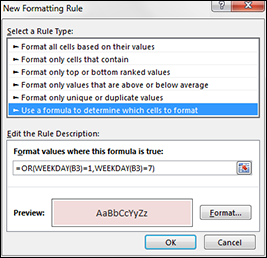
   Figure 9-10: Configure the New Formatting Rule dialog box to apply the needed formula rule.

   If you need to edit your conditional formatting rule, simply place your cursor in any of the data cells within your formatted range and then go to the Home tab and select Conditional Formatting⇒Manage Rules. This opens the Conditional Formatting Rules Manager dialog box. Click the rule you want to edit and then click the Edit Rule button.

Formula 98: Highlight Days between Two Dates

Some analysis requires the identification of dates that fall within a certain time period. Figure 9-11 demonstrates how you can apply conditional formatting that highlights dates based on a start date and end date. As you adjust the start and end dates, the conditional formatting adjusts with them.

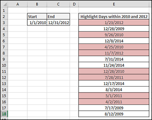
Figure 9-11: You can conditionally format dates that fall between a start and end date.

How it works

To build this basic formatting rule, follow these steps:

1. Select the data cells in your target range (cells E3:E18 in this example), click the Home tab of the Excel Ribbon, and then select Conditional Formatting⇒New Rule. This opens the New Formatting Rule dialog box shown in Figure 9-12.
2. In the list box at the top of the dialog box, click the Use a Formula to Determine which Cells to Format option. This selection evaluates values based on a formula you specify. If a particular value evaluates to TRUE, the conditional formatting is applied to that cell.
3. In the formula input box, enter the formula shown with this step. Note that you use the AND function to compare the date in your target cell (E3) to both the start and end dates found in cells $B$3 and $C$3, respectively. If the target cell falls within the start and end dates, the formula will evaluate to TRUE, thus triggering the conditional formatting.

   =AND(E3>=$B$3,E3<=$C$3)

   Note that in the formula, you exclude the absolute reference dollar symbols ($) for the target cell (E3). If you click cell E3 instead of typing the cell reference, Excel automatically makes your cell reference absolute. It’s important that you don’t include the absolute reference dollar symbols in your target cell because you need Excel to apply this formatting rule based on each cell’s own value.

   For more detail on the AND function, see Formula 46: Check Whether Condition1 AND Condition2 Are Met, in Chapter 5.

4. Click the Format button. This opens the Format Cells dialog box, where you have a full set of options for formatting the font, border, and fill for your target cell. After you have completed choosing your formatting options, click the OK button to confirm your changes and return to the New Formatting Rule dialog box.
5. Back in the New Formatting Rule dialog box, click the OK button to confirm your formatting rule.

   

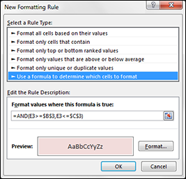
   Figure 9-12: Configure the New Formatting Rule dialog box to apply the needed formula rule.

   If you need to edit your conditional formatting rule, simply place your cursor in any of the data cells within your formatted range and then go to the Home tab and select Conditional Formatting⇒Manage Rules. This opens the Conditional Formatting Rules Manager dialog box. Click the rule you want to edit and then click the Edit Rule button.

Formula 99: Highlight Dates Based on Due Date

In many organizations, it’s important to call attention to dates that fall after a specified time period. With conditional formatting, you can easily create a “past due” report highlighting overdue items. The example shown in Figure 9-13 demonstrates a scenario where the dates that are more than 90 days overdue are formatted in red.

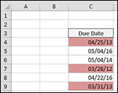
Figure 9-13: You can conditionally format dates based on due date.

How it works

To build this basic formatting rule, follow these steps:

1. Select the data cells in your target range (cells C4:C9 in this example), click the Home tab of the Excel Ribbon, and then select Conditional Formatting⇒New Rule. This opens the New Formatting Rule dialog box shown in Figure 9-14.
2. In the list box at the top of the dialog box, click the Use a Formula to Determine which Cells to Format option. This selection evaluates values based on a formula you specify. If a particular value evaluates to TRUE, the conditional formatting is applied to that cell.
3. In the formula input box, enter the formula shown here. In this formula, you evaluate whether today’s date is greater than 90 days past the date in your target cell (C4). If so, the conditional formatting will be applied.

   =TODAY()-C4>90

   Note that in the formula, you exclude the absolute reference dollar symbols ($) for the target cell (C4). If you click cell C4 instead of typing the cell reference, Excel will automatically make your cell reference absolute. It’s important that you don’t include the absolute reference dollar symbols in your target cell because you need Excel to apply this formatting rule based on each cell’s own value.

4. Click the Format button. This opens the Format Cells dialog box, where you have a full set of options for formatting the font, border, and fill for your target cell. After you have completed choosing your formatting options, click the OK button to confirm your changes and return to the New Formatting Rule dialog box.
5. Back in the New Formatting Rule dialog box, click the OK button to confirm your formatting rule.

   If you need to edit your conditional formatting rule, simply place your cursor in any of the data cells within your formatted range and then go to the Home tab and select Conditional Formatting⇒Manage Rules. This opens the Conditional Formatting Rules Manager dialog box. Click the rule you want to edit and then click the Edit Rule button.

   

   Figure 9-14: Configure the New Formatting Rule dialog box to apply the needed formula rule.

Formula 100: Highlight Data Based on Percentile Rank

A percentile rank indicates the standing of a particular data value relative to other data values in a sample. Percentiles are most notably used in determining performance on standardized tests. If a child scores in the 90th percentile on a standardized test, this means that his or her score is higher than 90 percent of the other children taking the test. Another way to look at it is to say that the child’s score is in the top 10 percent of all the children taking the test.

Percentiles are often used in data analysis as a method of measuring a subject’s performance in relation to the group as a whole — for instance, determining the percentile ranking for each employee based on an annual revenue.

In Excel, you can easily get key percentile ranks using the PERCENTILE function. This function requires two arguments: a range of data and the percentile score you want to see.

In the example shown in Figure 9-15, the value in cell D7 is a result of the following formula, which pulls the 75th percentile based on the data in range B3:B20:

=PERCENTILE($B$3:$B$20,0.75)

This formula tells you that any employee with revenue over $52,651 is in the top 75 percent of performers.

The value in cell D16 is a result of the following formula, which pulls the 25th percentile based on the data in range B3:B20:

=PERCENTILE($B$3:$B$20,0.25)

This formula tells you that any employee with revenue below $24,656 is in the bottom 25 percent of performers.

Using these percentile markers, this example applies conditional formatting so that any value in the 75th percentile will be colored green and any value in the 25th percentile will be colored red.

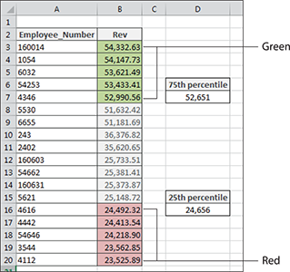
Figure 9-15: Using Excel’s PERCENTILE function to color code performance.

How it works

To build this basic formatting rule, follow these steps:

1. Select the data cells in your target range (cells B3:B20 in this example), click the Home tab of the Excel Ribbon, and then select Conditional Formatting⇒New Rule. This opens the New Formatting Rule dialog box shown in Figure 9-16.
2. In the list box at the top of the dialog box, click the Use a Formula to Determine which Cells to Format option. This selection evaluates values based on a formula you specify. If a particular value evaluates to TRUE, the conditional formatting is applied to that cell.
3. In the formula input box, enter the formula shown with this step. In this formula, you evaluate whether the data in the target cell (B3) is within the 25th percentile. If so, the conditional formatting will be applied.

   =B3<=PERCENTILE($B$3:$B$20,0.25)

   Note that in the formula, you exclude the absolute reference dollar symbols ($) for the target cell (B3). If you click cell B3 instead of typing the cell reference, Excel automatically makes your cell reference absolute. It’s important that you don’t include the absolute reference dollar symbols in your target cell because you need Excel to apply this formatting rule based on each cell’s own value.

4. Click the Format button. This opens the Format Cells dialog box, where you have a full set of options for formatting the font, border, and fill for your target cell. After you have completed choosing your formatting options, click the OK button to confirm your changes and return to the New Formatting Rule dialog box.
5. Back in the New Formatting Rule dialog box, click the OK button to confirm your formatting rule.

   

   Figure 9-16: Configure the New Formatting Rule dialog box to apply the needed formula rule.

6. At this point, you should be in the Conditional Formatting Rules Manager dialog box. Click the New Rule button.
7. This opens the New Formatting Rule dialog box shown in Figure 9-17. In the list box at the top of the dialog box, click the Use a Formula to Determine which Cells to Format option. This selection evaluates values based on a formula you specify. If a particular value evaluates to TRUE, then the conditional formatting is applied to that cell.
8. In the formula input box, enter the formula shown here. In this formula, you’re evaluating if the data in the target cell (B3) within the 75th percentile. If so, the conditional formatting will be applied.

   =B3>=PERCENTILE($B$3:$B$20,0.75)

9. Click the Format button. This opens the Format Cells dialog box, where you have a full set of options for formatting the font, border, and fill for your target cell. After you have completed choosing your formatting options, click the OK button to confirm your changes and return to the New Formatting Rule dialog box.
10. Back on the New Formatting Rule dialog box, click the OK button to confirm your formatting rule.

    

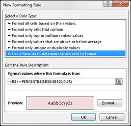
    Figure 9-17: Configure the New Formatting Rule dialog box to apply the needed formula rule.

    If you need to edit your conditional formatting rule, simply place your cursor in any of the data cells within your formatted range and then go to the Home tab and select Conditional Formatting⇒Manage Rules. This opens the Conditional Formatting Rules Manager dialog box. Click the rule you want to edit and then click the Edit Rule button.

Formula 101: Highlight Statistical Outliers

When performing data analysis, you usually assume that your values cluster around some central data point (a median). But sometimes a few of the values fall too far from the central point. These values are called outliers (they lie outside the expected range). Outliers can skew your statistical analyses, leading you to false or misleading conclusions about your data.

You can use a few simple formulas and conditional formatting to highlight the outliers in your data.

The first step in identifying outliers is to pinpoint the statistical center of the range. To do this pinpointing, you start by finding the 1st and 3rd quartiles. A quartile is a statistical division of a data set into four equal groups, with each group making up 25 percent of the data. The top 25 percent of a collection is considered to be the 1st quartile, whereas the bottom 25 percent is considered the 4th quartile.

In Excel, you can easily get quartile values by using the QUARTILE function. This function requires two arguments: a range of data and the quartile number you want.

In the example shown in Figure 9-18, the values in cells E3 and E4 are the 1st and 3rd quartiles for the data in range B3:B20.

Taking these two quartiles, you can calculate the statistical 50 percent of the data set by subtracting the 3rd quartile from the 1st quartile. This statistical 50 percent is called the interquartile range (IQR). Figure 9-18 displays the IQR in cell E5.

Now the question is, how far from the middle 50 percent can a value sit and still be considered a “reasonable” value? Statisticians generally agree that IQR*1.5 can be used to establish a reasonable upper and lower fence:

• The lower fence is equal to the 1st quartile – IQR*1.5.
• The upper fence is equal to the 3rd quartile + IQR*1.5.

As you can see in Figure 9-18, cells E7 and E8 calculate the final upper and lower fences. Any value greater than the upper fence or less than the lower fence is considered an outlier.

At this point, the conditional formatting rule is easy to implement.

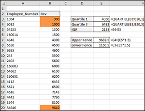
Figure 9-18: Highlighting outliers with conditional formatting.

For more detail on the quartile and interquartile ranges, see Formula 89: Identifying Statistical Outliers with an Interquartile Range, in Chapter 8.

How it works

To build this basic formatting rule, follow these steps:

1. Select the data cells in your target range (cells B3:B20 in this example), click the Home tab of the Excel Ribbon, and then select Conditional Formatting⇒New Rule. This opens the New Formatting Rule dialog box shown in Figure 9-19.

   

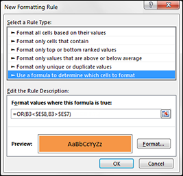
   Figure 9-19: Configure the New Formatting Rule dialog box to apply the needed formula rule.

2. In the list box at the top of the dialog box, click the Use a Formula to Determine which Cells to Format option. This selection evaluates values based on a formula that you specify. If a particular value evaluates to TRUE, the conditional formatting is applied to that cell.
3. In the formula input box, enter the formula shown here. Note that you use the OR function to compare the value in your target cell (B3) to both the upper and lower fences found in cells $E$7 and $E$8, respectively. If the target cell is greater than the upper fence or less than the lower fence, it’s considered an outlier and thus will evaluate to TRUE, triggering the conditional formatting.

   =OR(B3<$E$8,B3>$E$7)

   Note that in the formula, you exclude the absolute reference dollar symbols ($) for the target cell (B3). If you click cell B3 instead of typing the cell reference, Excel automatically makes your cell reference absolute. It’s important that you don’t include the absolute reference dollar symbols in your target cell because you need Excel to apply this formatting rule based on each cell’s own value.

4. Click the Format button. This opens the Format Cells dialog box, where you have a full set of options for formatting the font, border, and fill for your target cell. After you have completed choosing your formatting options, click the OK button to confirm your changes and return to the New Formatting Rule dialog box.
5. Back in the New Formatting Rule dialog box, click the OK button to confirm your formatting rule.

   If you need to edit your conditional formatting rule, simply place your cursor in any of the data cells within your formatted range and then go to the Home tab and select Conditional Formatting⇒Manage Rules. This opens the Conditional Formatting Rules Manager dialog box. Click the rule that you want to edit then click the Edit Rule button.