Chapter 6
Alignments

When working on a linear project, whether it be the renovation of an old New England cow path or a network of new subdivision roads, you will need to convey the horizontal layout information to the contractor. This horizontal layout is called an alignment and drives much of the design. This chapter teaches you how to create alignments, how they interact with the rest of the design, how to edit and analyze them, and finally how they work with the overall project.

In this chapter, you will learn to:

• Create an alignment from an object.
• Create a reverse curve that never loses tangency.
• Replace a component of an alignment with another component type.
• Create alignment tables.

Alignment Concepts

Before you can efficiently work with alignments, you must understand two major concepts: the interaction of alignments and sites and the idea of geometry that is fixed, floating, or free.

Alignments and Sites

Prior to the Autodesk^® AutoCAD^® Civil 3D^® 2008 release, alignments were always part of a site and interacted with the topology contained in that site. Civil 3D now has two ways of handling alignments in terms of sites: they can be contained in a site as before or they can be independent of a site (siteless).

There is no difference between the alignments contained in a site and those independent of a site since both can be used to cut profiles or control corridors, but only the alignments contained in a site will react with and create parcels as members of a site topology.

Unless you have good reason for them to interact, it makes sense to create alignments outside of any Site object. They can be moved later to a site if necessary. For the purpose of the exercises in this chapter, you won't place any alignments in a site. For more information about sites, check out the section “Introduction to Sites” in Chapter 5, “Parcels.”

Alignment Entities

Civil 3D recognizes five types of alignments: centerline alignments, offset alignments, curb return alignments, rail alignments, and miscellaneous alignments. Each alignment type can consist of three types of entities, or segments: lines, arcs, and spirals. These segments control the horizontal alignment of your design. Their relationship to one another is described by the following terminology:

1. Fixed Segments Fixed segments are fixed in space (see Figure 6.1). They're defined by connecting points in the coordinate plane and are independent of the segments that occur either before or after them in the alignment. Fixed segments can be created as tangent to other components, but their independence from those objects lets you move them out of tangency during editing operations. An alignment that is defined from lines and arcs will have its segments fixed. If the lines on both sides of the arcs are tangents, they will be defined as free segments.

   

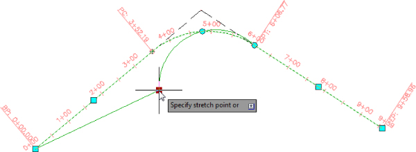
   Figure 6.1 Alignment fixed segments

2. Floating Segments Floating segments float in space but are attached to a point in the drawing and to a single segment to which they maintain tangency (see Figure 6.2). Floating segments work well in situations where you have a critical point but the other points of the horizontal alignment are flexible.

   

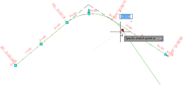
   Figure 6.2 Alignment floating segments

3. Free Segments Free segments are dependent upon the entities that come both before and after them in the alignment structure (see Figure 6.3). Unlike fixed or floating segments, a free segment must have segments that come before and after it. Free segments maintain tangency to the segments that come before and after them and move as required to make that happen. Although some geometry constraints can be put in place, these constraints can be edited and are user dependent. As a note, the alignment that is created from a polyline will be defined by free segments only if the segments before and after an Arc object are tangents; otherwise, the segments will be fixed, as mentioned previously.

   

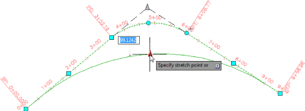
   Figure 6.3 Alignment free segments

During the exercises in this chapter, you'll use a mix of these entity types to understand them better.

Creating an Alignment

You can create alignments using the following methods:

1. From Objects You will likely use this method to convert an existing centerline made out of arcs and lines or polylines to an Alignment object. With this method, you can also pull these types of entities from an attached external reference.
2. By Layout The tools available under this method allow you to both define an alignment using dynamic line and curve elements and edit alignments created using all the other methods.
3. Best Fit This method is used to define an alignment using as input data a selection of AutoCAD blocks, entities, points, COGO points, or feature lines. Based on specific constraints, a best-fitted Alignment object is created.
4. Offsets These alignments define offset alignments that use a common centerline alignment as the source to which they are dynamically linked.
5. Widening Widening alignments are based on either centerline or offset alignments and are dynamic linked to them. They are used in the definition of a road widening in a road corridor model.
6. From Corridor This method allows a user to create an alignment using a corridor feature line.
7. From Network Parts This method allows the creation of an alignment using the selection of a series of pipes and structures that belong to a Civil 3D pipe network.
8. From Pressure Network This method allows the creation of an alignment using a selection of pipes, fittings, and appurtenances that belong to a Civil 3D pressure pipe network.
9. Using Existing Alignment This method allows the creation of an alignment using a previously defined alignment object as source.

This section looks at the first four methods to create an alignment, outlining some of the advantages and disadvantages of each. The remaining methods are straightforward, and once you master the methods used in this section, you should not have any issues in mastering them as well. The exercise will use the street layout shown in Figure 6.4 as well as the different methods to achieve your designs.

Figure 6.4 Proposed street layout

Creating from a Line, Arc, or Polyline

Most designers have used either polylines or lines and arcs to generate the horizontal control of their projects. It's common for surveyors to generate polylines to describe the center of a right-of-way or for an environmental engineer to draw a polyline to show where a new channel should be constructed. These team members may or may not have Civil 3D software, so they use their familiar tools—the line, arc, and polyline—to describe their design intent.

Although these objects are good at showing where something should go, they don't have much data behind them. To make full use of these objects, you should convert them to Civil 3D alignments that can then be shared and used for myriad purposes. Once an alignment has been created from a polyline, offsets can be created to represent rights-of-way, building lines, and so on. In the following exercise, you'll convert a polyline to an alignment and create offset alignments:

1. Open the 0601_AlignmentFromObjects.dwg (0601_AlignmentFromObjects_METRIC.dwg) file.

   You can download this file from the book's web page at www.sybex.com/go/masteringcivil3d2015. You will see a polyline that represents the centerline of a proposed road together with the parcels that you got familiar with in Chapter 5.
   

2. From the Home tab Create Design panel, choose Alignment Create Alignment From Objects.
3. When prompted to select the first line, pick the polyline that defines the centerline near its north end, and press ↲ .
4. At the Press enter to accept alignment direction or [Reverse]: prompt, press ↲ once you confirm that the displayed arrow outlining the direction points from north to south.

   The Create Alignment From Objects dialog appears.

5. Change the Name field to ROAD D, and set the Type field to Centerline from the drop-down list.
6. Verify that Alignment Style is set to Proposed, and Alignment Label Set is set to Major And Minor Only.
7. Within Conversion Options, make sure that the Add Curves Between Tangents option is unchecked, and the Erase Existing Entities box is checked.

   The Create Alignment From Objects dialog should match Figure 6.5.

8. Accept the other settings and click OK.

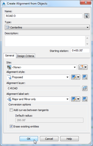
Figure 6.5 The settings used to create the ROAD D alignment

When this exercise is complete, you may save the drawing, but keep it open for the following exercise. A finished copy of this drawing at this stage is available from the book's web page with the filename 0601_AlignmentFromObjects_A.dwg (0601_AlignmentFromObjects_A_METRIC.dwg).

---

A Word About Constraints

Prior to the 2014 release, creating from objects held no constraints (everything was fixed). In current versions, Civil 3D tries to find tangency where a curve is between two lines and establish that tangency as a constraint. Lines will always be set to Not Constrained (Fixed), but if the curve is tangent, it will be set to Constrained On Both Sides (Free). You will learn about changing those constraints later in this chapter.

---

---

The Create Alignment From Objects Dialog

In the Create Alignment From Objects dialog (shown in Figure 6.5), there are many settings that you can adjust when creating an alignment:

1. Name This is the alignment name. No alignment name can be duplicated in a drawing. When an alignment name is found to be a duplicate, a modifier is added to its name to show that difference.
2. Type The alignment types can be thought of as places for objects that are alike. The objects can react differently depending on which type is selected.
   1. Centerline Used mainly for centers of roads, streams, or swales. Civil 3D places this type of alignment in the Alignments Centerline Alignments branch.
   2. Offset Used for offset alignments. The difference between this and the centerline alignment is that you have the option in the Alignment Properties dialog to set Offset parameters, such as naming a parent alignment and offset values. Offset alignments are dynamically linked to their parent alignments and will update automatically when the parent alignment changes. Civil 3D places this type of alignment in the Alignments Offset Alignments branch.
   3. Curb Return Used for curb returns, which are the radii at intersections. The difference between this and the offset alignment is that instead of Offset parameters, you have the option in the Alignment Properties dialog to set Curb Return parameters, such as setting two parent alignments and offsets. Curb return alignments are also dynamically linked to their parent alignments. Civil 3D places this type of alignment in the Alignments Curb Return Alignments branch.
   4. Rail Used for rail design. The difference between this and the other alignments is that this alignment is set using typical rail geometry such as degree of curvature and cant. In addition, a unique tab is added to the Alignment Properties dialog called Rail Parameters, where you can specify the track width. Civil 3D places this alignment type in the Alignments Rail Alignments branch.
   5. MiscellaneousThis is a stripped-down alignment type that contains only Information, Stationing, Masking, Point Of Intersection, and Constraint Editing tabs. Civil 3D places this alignment type in the Alignments Miscellaneous Alignments branch.
   6. Description This is an optional field where you can place the description of what your alignment represents.
   7. Starting Station This value, either positive or negative, will be the starting stationing for the alignment. This is handy if you need to start your alignment to coincide with existing stationing or if you want to have your 0+00 stationing at an intersection of a road. If you forget to set this value here, you can change it later in the Alignment Properties dialog.

The General tab contains the following options:

1. Site This is a place to keep Civil 3D objects that you want to interact with each other. As previously mentioned, all of your alignments in these exercises will be put on the <None> site.
2. Alignment Style You can set different styles to visually show your alignment. For more on styles, refer to Chapter 19, “Object Styles.”
3. Alignment Layer This setting overrides the layer that is specified in the drawing settings for the alignment that you create.
4. Alignment Label Set As with the Alignment Style, you can choose how your alignment will be labeled. For more on label styles, refer to Chapter 18, “Label Styles.”
5. Conversion Options Depending on your selections, these will add curves and/or erase the original entities, or neither.

The Design Criteria tab contains these options:

1. Starting Design Speed Use this option to specify the design speed of the alignment for the starting station. If no additional design speeds are applied to a different section of the alignment, this speed will be used for the entire alignment. Design speed is used to calculate superelevation and to establish design criteria.
2. Use Criteria-Based Design When this check box is selected, the Use Design Criteria File and Use Design Check Set options are available. These options enable the software to keep track of certain design standards that you would like your alignment to meet and notify you when those standards are not met.
3. Use Design Criteria File Here you can define the design criteria, as it is defined in the design manual A Policy on Geometric Design of Highways and Streets, 2011 from the American Association of State Highway and Transportation Officials (AASHTO).
4. Use Design Check Set Here you can set rules or expressions for lines, curves, spirals, and tangent intersections.

Many of these settings will be discussed further throughout this chapter.

---

You've created your first alignment and attached stationing and major and minor labels. It is common to create offset alignments from a centerline alignment to begin to model rights-of-way. In the following exercise, you'll create offset alignments and mask them where you don't want them to be seen:

1. Continue working on the previous file, or if you want to begin from the previous step, you can open the 0601_AlignmentFromObjects_A.dwg (0601_AlignmentFromObjects_A_METRIC.dwg) file.
   
2. From the Home tab Create Design panel, choose Alignment Create Offset Alignment option.
3. When prompted to select an alignment, pick the ROAD D alignment to open the Create Offset Alignments dialog shown in Figure 6.6.

   

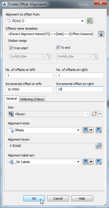
   Figure 6.6 The Create Offset Alignments dialog

4. With No. Of Offsets On Left set to 1, change Incremental Offset On Left to 30 (metric users, 10).
5. With No. Of Offsets On Right set to 1, change Incremental Offset On Right to 30 (metric users, 10).
6. Verify that Alignment Label Set is set to _No Labels and click OK to accept the rest of the defaults shown in Figure 6.6.
7. Select the left offset alignment just created along the easterly and northerly right-of-way of ROAD D to activate the Offset Alignment contextual tab.
8. From the Offset Alignment contextual tab Modify panel, click the Alignment Properties icon to open the Alignment Properties dialog.
9. Change to the Masking tab and click the Add Masking Region button.
   
10. Enter 264.90 for the first station and 326.47 for the second station when prompted (metric users, enter 81.46 and 98.78) and click OK. Alternatively, you could have used the station picker that becomes available once the station cell is active and in editing mode.
    

    Notice that the alignment is now masked at the intersection of the alignment with the right-of-way at the north end.

11. Repeat the process for the rest of the intersections for both of the offset alignments by using the station picker and snapping to the intersection of the offset alignments and the right-of-way lines so that the areas in between the right-of-way lines are masked.

    Once complete, the Masking tab of the Alignment Properties dialog should look like Figure 6.7 for the case of the left offset.

    

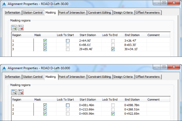
    Figure 6.7 Creating an alignment mask for the left offset with both U.S. (top) and metric (bottom) values.

12. Click OK to close the dialog.

    Offset alignments are simple to create, and they are dynamically linked to a centerline alignment.

13. To test this, grip the centerline alignment, select the endpoint grip, and stretch the alignment to the west.

    Notice the change and then undo this change to return to the original state.

---

Offset Grips and More

Offset alignments have two main grips: the arrow and the plus sign. The arrow is used to change the offset value, and the plus sign is used to create a transition, called a widening, such as a turning lane. When a widening is present, there will be a third grip present in the form of a filled gray circle that enables the transition grips. To access the Create Widening command, from the Home tab Create Design panel, select the Alignment drop-down. Widening criteria can also be found in the Create Offset Alignments dialog and the Offset Alignment contextual tab. The widening in the Offset Alignments contextual tab can be added as a new alignment or as an element within the existing offset alignment.

Also, offset alignments with widening remain dynamic to their host alignment. Offset alignment objects can be found in Prospector in the Alignments branch.

---

When this exercise is complete, you can close the drawing. A finished copy of this drawing is available from the book's web page with the filename 0601_AlignmentFromObjects_FINISHED.dwg (0601_AlignmentFromObjects_METRIC_FINISHED.dwg).

Creating by Layout

Now that you've made an alignment from polylines, let's look at another creation option: Create By Layout. You'll use the same street layout (Figure 6.4) that was provided by a planner, but instead of converting from polylines, you'll trace the alignments. Although this seems like duplicate work, it will pay dividends in the relationships created between segments.

1. Open the 0602_AlignmentByLayout.dwg (0602_AlignmentByLayout_METRIC.dwg) file.
2. From the Home tab Create Design panel, choose the Alignment Alignment Creation Tools option.
   

   The Create Alignment – Layout dialog appears.

3. Change the Name field to ROAD D if it is not already set.
4. Verify that Alignment Style is set to Proposed and Alignment Label Set is set to Major And Minor Only.
5. Click OK to accept the other settings shown in Figure 6.8.

   

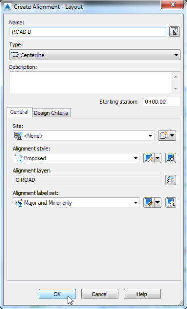
   Figure 6.8 Create Alignment – Layout dialog

   The Alignment Layout Tools toolbar for ROAD D appears (Figure 6.9).

   

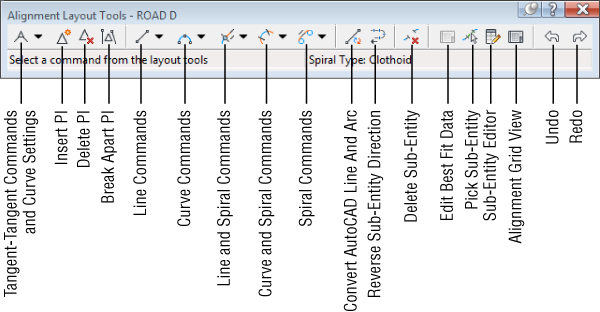
   Figure 6.9 The Alignment Layout Tools toolbar for the ROAD D alignment

6. Click the down arrow next to the Tangent-Tangent (No Curves) tool at the far left and select the Tangent-Tangent (With Curves) option (see Figure 6.10).

   

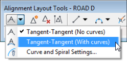
   Figure 6.10 The Tangent-Tangent (With Curves) tool

   This tool places a curve automatically based on a default setting that is defined under the Curve And Spiral Settings option from the same menu. Later, you'll adjust the curve based on your design's preferred layout.

7. Turn on the Endpoint Osnap and snap to the north endpoint of the ROAD D centerline.
8. Continue to pick the vertices endpoints of the red polyline along the ROAD D centerline, from north to south and then east to finish creating this alignment.
9. After selecting the last endpoint along the red polyline, press ↲ to end the command.
10. Click the X button at the upper right on the Alignment Layout Tools toolbar for ROAD D to close it.

    Keep this drawing open for the next portion of the exercise.

    Zoom in around the areas with arcs. Notice that some of them follow very closely the desired layout, while others are off by a huge margin from what the planner envisioned as design parameters for those arcs. That's okay—you will fix them in a later exercise.

    The alignment you just made is one of the most basic. Let's create additional alignments and use a few of the other tools to complete your initial layout. In this exercise, you will build the alignment at the center of the site that will access the cul-de-sac area, but this time you will use a floating curve to ensure the two segments you will be creating maintain their relationship.

    ---

    Design and Then Refine

    It bears repeating that when creating Civil 3D objects, it is good practice to get something in place and then refine it. With Land Desktop or other packages, you didn't want to define the object until it was fully designed. In Civil 3D, you define the object in a preliminary state and then refine your design.

    ---

11. From the Home tab Create Design panel, choose Alignment Alignment Creation Tools.

    The Create Alignment – Layout dialog appears.

12. In the Create Alignment – Layout dialog, do the following:
    1. Change the Name field to ROAD G.
    2. Set the Alignment Style field to Proposed.
    3. Set the Alignment Label Set field to Major And Minor Only.
13. Click OK to display the Alignment Layout Tools toolbar for ROAD G.
14. Select the Fixed Line (Two Points) tool, as shown in Figure 6.11.

    

    Figure 6.11 The Fixed Line (Two Points) tool

15. At the Specify start point: prompt, using Endpoint Osnap, select the north endpoint of the polyline, and working north to south, draw the first fixed-line segment to the south end of the segment.

    When you've finished, the command line will read Specify start point: in case you want to draw another line. You can either press ↲ to end the command or draw the next entity without ending the command.

16. Click the down arrow next to the Add Fixed Curve (Three Point) tool on the toolbar and select More Floating Curves Floating Curve (From Entity End, Through Point), as shown in Figure 6.12.

    

    Figure 6.12 Selecting the Floating Curve tool

17. At the Select entity to attach to: prompt, select the fixed-line segment you drew in steps 14 and 15.

    Make sure you select the line segment somewhere south of the segment's midpoint to connect to the southern endpoint instead of the northern endpoint. If you cannot select the alignment segment, enable Selection Cycling (Ctrl+W).

18. At the Specify Pass Through Point: prompt, pick the endpoint between the two arcs (the point of compound curvature).

    Notice that you are generating the segments from low station to high station. If you perform these steps backward, you can reverse a segment using the Reverse Sub-Entity Direction button on the Alignment Layout Tools toolbar.

19. Use the same command to draw the last arc segment, using the previous alignment arc segment as your entity to attach and the end of the polyline as the through point.
20. Press ↲ to end the command.
21. Close the Alignment Layout Tools toolbar.
22. Pick the ROAD G alignment and then pick the grip on the lower end of the line and pull it away from its location.

    Notice that the line and the arcs are in sync and tangency is maintained (see Figure 6.13).

    

    Figure 6.13 Floating curves maintain their tangency.

23. Press Esc to cancel the grip edit.

When this exercise is complete, you can close the drawing. A finished copy of this drawing is available from the book's web page with the filename 0602_AlignmentByLayout_FINISHED.dwg (0602_AlignmentByLayout_METRIC_FINISHED.dwg).

---

All Aboard! Rail Alignments

Rail alignments were introduced in Civil 3D 2013 to allow for the differences between rail design and other types of design. For example, railways are characterized by long sweeping curves, and the curve geometry is expressed differently on railway construction plans. Rail design also has its own type of superelevation called cant, which is handled differently than road superelevation. These differences are accounted for when you use rail alignments in Civil 3D. Let's look at a quick, simple example:

1. Start a new blank drawing from the _AutoCAD Civil 3D (Imperial) NCS template that ships with Civil 3D. Metric users should use the _AutoCAD Civil 3D (Metric) NCS template.
2. From the Home tab Create Design panel, choose the Alignment section Alignment Creation Tools option.

   The Create Alignment – Layout dialog appears.

3. Change the name to Mastering Railway and set Type to Rail.
4. On the General tab, make these changes:
   • Set Alignment Style to Proposed.
   • Set Alignment Label Set to All Labels.
5. Switch to the Design Criteria tab.
6. Change the starting design speed to 30 mi/hr (or 50 km/hr for metric users).
7. Select the Use Criteria-Based Design check box.

   If the design criteria file doesn't default to the one that references railway design standards, you may need to click the ellipsis next to the design criteria file, which by default shows _Autodesk Civil 3D Imperial Rail Cant Design Standards.xml or _Autodesk Civil 3D Metric Rail Cant Design Standards.xml available to select and use.

8. Verify that Use Design Criteria File and Use Design Check Set are also checked.
9. Click OK.

   The Alignment Layout Tools toolbar appears.

10. Select the Fixed Line (Two Points) tool.
11. Click anywhere on the screen to define the start point, and define the second point by entering @330,0 on the command line (or @100,0 for metric users).
12. Press ↲ to end the command.
13. From the More Floating Curves branch, select Floating Curve (From Entity End, Radius, Length).
14. At the Select entity to attach to: prompt, select the right side of the line segment that you just drew.
15. At the Specify curve direction [Clockwise cOunterclockwise] <Clockwise>: prompt, press ↲ to accept the default, Clockwise.
16. At the Specify radius or [Degree of curvature]: prompt, enter D ↲ to switch to entering the radius by degree of curvature.
17. At the Specify degree of curvature or [Radius]: prompt, enter 3 ↲.
18. At the Specify curve length or [deltaAngle Tanlen Chordlen midOrd External]: prompt, enter C ↲ to define by chord length.
19. At the Specify chord length or [curveLen deltaAngle Tanlen midOrd External]: prompt, enter 100 ↲.
20. Press ↲ to end the command. Click the X on the corner to close the Alignment Layout Tools toolbar.

Note that this will result in a different curve for Imperial and metric users.

When this exercise is complete, you can close the drawing. A saved finished copy of this drawing is available from the book's web page with the filename 0603_RailAlignment_FINISHED.dwg (0603_RailAlignment_METRIC_FINISHED.dwg).

---

Best-Fit Alignments

Often designers have to re-create an alignment for an existing road that does not have defined horizontal geometry. Civil 3D has multiple tools to re-create the alignment using a best-fit algorithm. You can either re-create a full best-fit alignment or use best-fit lines or best-fit curves in an alignment. You will look at both methods to achieve this within the following section.

The Create Best Fit Alignment command can use AutoCAD blocks, AutoCAD entities, AutoCAD points, Civil 3D COGO points, or Civil 3D feature lines. You can also pick points by simply clicking the screen. The Line and Curve drop-down menus on the Alignment Layout toolbar include options for Floating and Fixed Lines By Best Fit as well as Best Fit curves in all three flavors: Fixed, Float, and Free. It is similar to what was covered in Chapter 1, “The Basics,” in the section “Best-Fit Entities.” Let's see how it works with alignments:

1. Open the 0604_AlignmentBestFit.dwg (0604_AlignmentBestFit_METRIC.dwg) file, which you can download from this book's web page.
2. From the Home tab Create Design panel, choose the Alignment section Alignment Creation Tools option.

   The Create Alignment – Layout dialog appears.

3. Enter Best Fit Lines in the Name field.
4. Leave the rest at their defaults and click OK.

   The Alignment Layout Tools toolbar opens.

5. Click the down arrow next to the Fixed Line (Two Points) tool on the toolbar and select the Fixed Line – Best Fit option.

   The Tangent By Best Fit dialog opens (Figure 6.14).

   

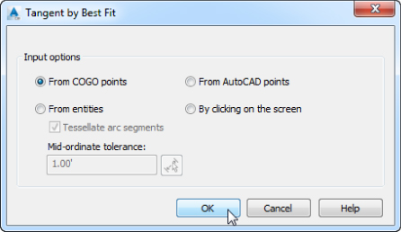
   Figure 6.14 The Tangent By Best Fit dialog

   Here, you can choose various methods to create a best-fit line alignment:

   • From COGO Points
   • From Entities
   • From AutoCAD Points
   • By Clicking On The Screen
6. Pick the From COGO Points radio button and click OK.

   At the Select Point objects or [Numbers Groups]: prompt, select points 1–11 using a combination of selection on the screen and transparent commands.

7. On point selection, select manually points 1 to 6.
8. When it comes to select the point 7, at the command line enter the transparent command for point number: 'pn ↲. In the point number selection, enter 7-11 ↲. Press the Esc key once to exit transparent mode.

   As you continue defining the tangent, you will see a red dashed line being formed. In your selections, this line looks at all the endpoints selected in order to create the best-fit line alignment segment (Figure 6.15).

   

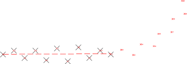
   Figure 6.15 The best-fit line being formed

9. Press ↲ to open the Regression Data tab of the Panorama window shown in Figure 6.16.

   

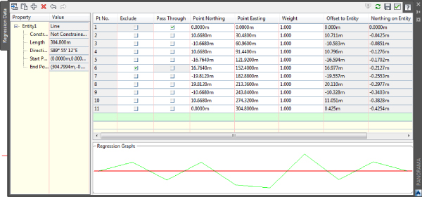
   Figure 6.16 Regression Data tab of the Panorama window

   On the Regression Data tab of the Panorama window, you can choose to exclude endpoints or force them to be pass-through endpoints by checking the appropriate boxes.

   As you check and uncheck boxes in the Regression Data chart, notice the changes that occur on your best-fit line alignment.

10. For this exercise you will try to make sure that the line will pass through point 1 and exclude point 6. Therefore, put a check mark in the Pass Through check box for point 1 and one in the Exclude check box for point 6, as shown in Figure 6.16.
11. Click the green check mark on the upper-right side of Panorama to accept the selection and dismiss the Panorama window.

    You will notice that the line is drawn temporarily until you click the green check mark and exit the Panorama window or if you are still in the Panorama window, when you click the Save button.

12. Without exiting the Alignment Layout Tools toolbar, you will build a best-fit floating curve using the remainder of COGO points. Expand the curve creation tools and select the Floating Curve – Best Fit option, as shown in Figure 6.17.

    

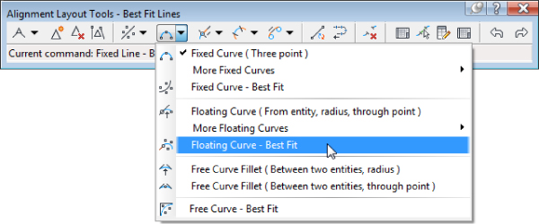
    Figure 6.17 The Floating Curve – Best Fit option

13. At the Select entity to attach to: prompt, select the previously defined segment close to the right end.

    The Curve By Best Fit dialog appears.

14. Select the From COGO Points option and click OK.
15. At the Select point objects or [Number Groups]: prompt, enter G and press ↲ to select a point group.

    The Point Groups Selection dialog will appear.

16. Select the Curve Point Group and click OK. You will notice the curve being created and the Regression Data tab appearing again, this time for the curve (see Figure 6.18).

    

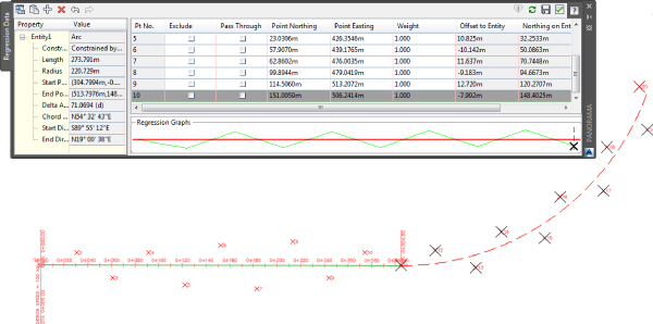
    Figure 6.18 The floating curve temporary layout and Regression Data tab of the Panorama window

17. Click the green check mark to finish the creation of the curve and click the X on the toolbar to exit the creation of the alignment workflow.

    The best-fit line alignment is complete.

    Keep this drawing open for the next portion of the exercise.

    One of the benefits of doing individual best-fit segments (lines or curves) is that it is easy to exclude points. However, sometimes you will want a single “rough and dirty” alignment full of curves and lines without having to define them individually. Next, you will create a full best-fit alignment.

    For the creation of the full best-fit alignment, you will use the same COGO points that you used for the first part of the exercise. You will do this in order to compare the results of both methods. If you create segments using best-fit line or best-fit curve, for example, you can use the Edit Best Fit Data For All Entries tool to edit these segments after they are created.
    

18. From the Home tab Create Design panel, choose the Alignment section Create Best Fit Alignment.

    The Create Best Fit Alignment dialog appears.

19. Set the input type to COGO Points; on the drop-down list of Path 1 Point Group, select the _All Points point group.
20. Deselect the Create Spirals check box.
21. Change Alignment Name to Best Fit Alignment.
22. Verify that Alignment Style is set to Layout, Alignment Label Set is set to _No Labels, and the Show Report box is checked, as shown in Figure 6.19. Then click OK to accept all the other defaults.

    

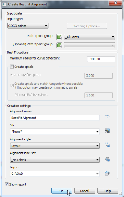
    Figure 6.19 The Create Best Fit Alignment dialog

    The Best Fit Report dialog opens, as shown in Figure 6.20.

    

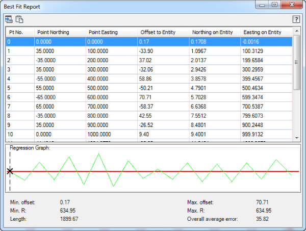
    Figure 6.20 The Best Fit Report dialog

    Review the results in the Best Fit Report. Notice that if you select a row, it will highlight the location on the regression graph.

23. Click the close (X) button to dismiss the dialog.

Unlike the Regression Data tab in the Panorama window, the Best Fit Report is purely informational and does not allow you to select to exclude or pass through a specific point. While the Create Best Fit Alignment procedure is fast, it may not be precise. Therefore, this command may be useful for providing a draft alignment, and then you can manually create your final alignment using results similar to those shown in the Best Fit Report that meet your specific design criteria.

The completed best-fit alignment is shown together with the alignment made with the best-fit lines and curves in Figure 6.21. Although a best-fit alignment may not give you exactly what you are looking for (especially if you like nice, whole-number radii), it generates a good starting point that you can then edit to fit your design needs.

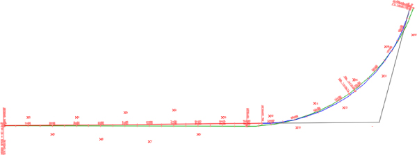
Figure 6.21 The best-fit alignment

When this exercise is complete, you can close the drawing. A finished copy of this drawing is available from the book's web page with the filename 0604_AlignmentBestFit_FINISHED.dwg (0604_AlignmentBestFit_METRIC_FINISHED.dwg).

Reverse and Compound Curve Creation

Next, let's look at a more complicated alignment—building reverse and compound curves by connecting two curves:

1. Open the 0605_ReverseCompoundAlignment.dwg (0605_ReverseCompoundAlignment_METRIC.dwg) file.
2. For this exercise, confirm that your Endpoint Osnap is active using the Osnap settings since you will need to snap to endpoints for this exercise.

   Also, disable polar tracking.

3. From the Home tab Create Design panel, choose Alignment Alignment Creation Tools.

   The Create Alignment – Layout dialog appears.

4. In the Create Alignment – Layout dialog, do the following:
   1. Change the Name field to Reverse-Compound.
   2. Set the Alignment Style field to Layout.
   3. Set the Alignment Label Set field to Major Minor And Geometry Points.
5. Click OK to display the Alignment Layout Tools toolbar for the alignment.
   
6. Start by drawing a fixed line from the west endpoint heading east along the tangent to the place where this tangent meets the magenta arc, using the same Fixed Line (Two Points) tool as used in an earlier exercise. Do the same thing for the end tangent of the alignment, starting from the end of the cyan arc and finishing at the east endpoint of that tangent.
7. Press Enter to finish drawing the line segments.

   You will notice that the second segment will not have any labels applied to it, since it is not connected to the first segment created.
   

8. Use the Floating Curve (From Entity, Radius, Through Point) tool to connect a curve from the endpoint of the first drawn tangent.
9. At the Select entity to attach to: prompt, pick the right end of the west tangent. At the Specify radius or [Degree of curvature]: prompt, enter 200 ↲ (for metric, 60.96 ↲).
10. At the Is curve solution angle [Greaterthan180 Lessthan180] <Lessthan180>: prompt, press ↲ to accept the default.
11. At the Specify end point: prompt, click the other end of the arc, where the magenta arc meets the green arc.
12. The command repeats; at the Select entity to attach to: prompt, select the right side of the curve you just created.
13. At the Specify radius or [Degree of curvature]: prompt, enter 300 ↲ (for metric, 91.44 ↲).
14. At the Is curve solution angle [Greaterthan180 Lessthan180] <Lessthan180>: prompt, press ↲ to accept the default.

    The program detects that you are attaching a curve to a curve.

15. At the Is curve compound or reverse to curve before? [Compound Reverse] <Compound>: prompt, enter R ↲ to specify that it is a reverse curve.
16. At the Specify end point: prompt, click the endpoint of the second arc or the connecting point between the green and blue arcs.
17. The command repeats. Repeat steps 12–15, but enter 250 (for metric, 76.20) for a radius and choose Compound as the type of curve.
18. At the Specify end point: prompt, click the endpoint of the third arc or the connecting point between the blue and cyan arcs.
19. Press ↲ to end the command. You should be able to see the stationing through all the arcs you created so far.
    
20. For the final arc you will a conversion tool. Use the Convert AutoCAD Line And Arc tool to define the last arc segment that connects the previously defined curve to the second tangent segment. Click the tool, select the arc, and press ↲.

    You will notice that upon the connection of the last arc to the segment, the missing labels will be added to the tangent since now it is connected to the main chain. You can see the final result of the layout in Figure 6.22.

    

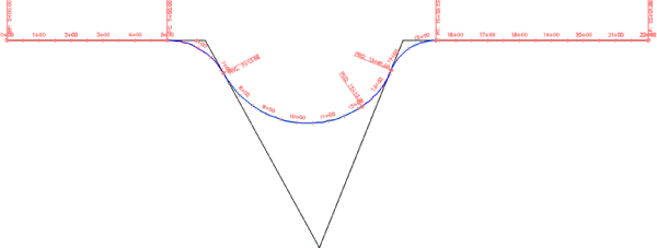
    Figure 6.22 Segment layout for the reverse and compound curve alignment

The alignment now contains a perfect series of reverse-compound-reverse curves. Move any of the pieces, and you'll see the other segments react to maintain the relationships shown in Figure 6.23. The flexibility of the Civil 3D tools allows you to explore an alternative solution (the reverse curve) as opposed to the basic solution. Flexibility is one of the strengths of Civil 3D.

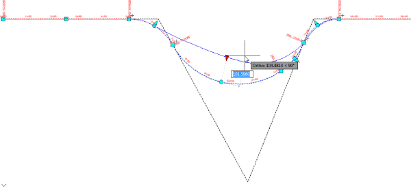
Figure 6.23 Curve relationships during a grip edit

You've completed your initial reverse and compound curve layout. Unfortunately, the curve design may not be acceptable to the designer, but you'll look at those changes later in the section “Component-Level Editing.”

When this exercise is complete, you can close the drawing. A finished copy of this drawing is available from the book's web page with the filename 0605_ReverseCompoundAlignment_FINISHED.dwg (0605_ReverseCompoundAlignment_METRIC_FINISHED.dwg).

Creating with Design Constraints and Check Sets

Civil 3D allows you to use design constraints and design check sets during the process of creating alignments and design profiles. Typically, these constraints check for things such as curve radius, length of tangents, and so on. Design constraints use information from AASHTO or other design manuals to set curve requirements. Check sets allow users to create their own criteria to match local requirements, such as subdivision or county road design. In this exercise, you'll make one quick set of design checks:

1. Open the 0606_AlignmentCheck.dwg (0606_AlignmentCheck_METRIC.dwg) file.
2. On the Settings tab in Toolspace, expand the Alignment Design Checks branch.
3. Right-click the Line category and select New to display the New Design Check dialog.
4. Change the name to Subdivision Tangent.
   
5. Click the Insert Property drop-down menu and select Length.
6. Click the greater-than/equals symbol (>=) button and then enter 100 (for metric, 30.48) in the Expression field, as shown in Figure 6.24.

   When complete, your dialog should look like Figure 6.24.

   

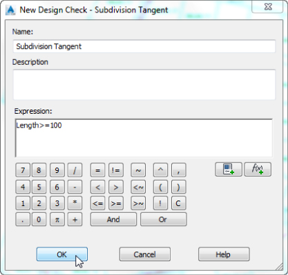
   Figure 6.24 The completed Subdivision Tangent design check

7. Click OK to accept the settings in the dialog.
8. Right-click the Curve category and select New to display the New Design Check dialog.
9. Change the name to Subdivision Radius.
10. Click the Insert Property drop-down menu and select Radius.
11. Click the greater-than/equals symbol (>=) button and then enter 200 (for metric, 60.96) in the Expression field, as shown in Figure 6.25.

    

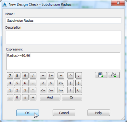
    Figure 6.25 The completed Subdivision Radius design check

12. Click OK to accept the settings in the dialog.
13. Right-click the Design Check Sets folder and select New to display the Alignment Design Check Set dialog.
14. On the Information tab, change the name to Mastering Subdivision and then switch to the Design Checks tab.
15. Choose Line from the Type drop-down list and select the Subdivision Tangent line check that you just created.
16. Click the Add button to add the Subdivision Tangent check to the set.
17. Choose Curve from the Type drop-down list and select the Subdivision Radius curve check that you just created.
18. Click the Add button again to complete the set, as shown in Figure 6.26.

    

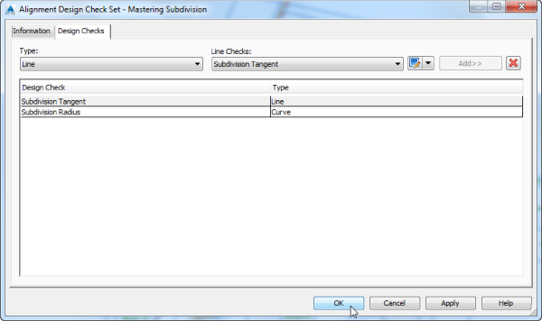
    Figure 6.26 The completed Mastering Subdivision design check set

19. Click OK to accept the settings in the dialog.

You can keep this drawing open to continue to the next exercise or use the finished copy of this drawing available from the book's web page 0606_AlignmentCheck_FINISHED.dwg (0606_AlignmentCheck_METRIC_FINISHED.dwg).

Once you've created a number of design checks and design check sets, you can apply them as needed during the design and layout stage of your projects.

---

Design Checks vs. Design Criteria

What's the difference between design checks and design criteria? A design check uses basic properties such as radius, length, grade, and so on, to check a particular portion of an alignment or profile. These constraints are generally dictated by a governing agency based on the type of road involved. Design criteria use speed and related values from design manuals such as AASHTO to establish these geometry constraints. Think of design criteria as a suite of check sets with different sets for each city, type of street, design speed, and so on.

---

In the next exercise, you'll see the results of your Mastering Subdivision check set in action:

1. If it's not still open from the previous exercise, open the 0606_AlignmentCheck_FINISHED.dwg (0606_AlignmentCheck_METRIC_FINISHED.dwg) file.
2. Change to the Prospector tab in Toolspace and expand the Alignments Centerline Alignments branches.
3. Right-click ROAD D and select Properties.
4. Change to the Design Criteria tab and set the start station design speed to 30 mi/h (or metric, 48 km/h), as shown in Figure 6.27.

   

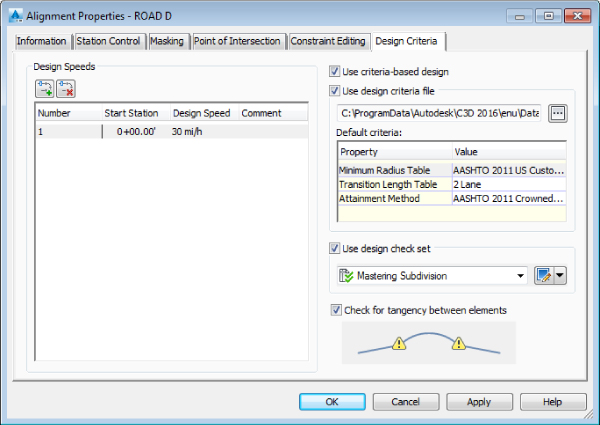
   Figure 6.27 Setting up design checks from Alignment Properties

5. Verify that all of the check boxes are selected and that Use Design Check Set is set to Mastering Subdivision, as shown in Figure 6.27.

   Note that the Use Criteria-Based Design check box must be selected to activate the other two.

6. Click OK to accept the settings in the dialog.

   You could have alternatively set the design criteria when you were originally creating the alignment.

   Notice that all the curves along the alignment fail to meet the design criteria.

   If you hover your cursor over one of the exclamation-point symbols, as shown in Figure 6.28, it will indicate which design criteria and design checks have been violated. Make sure you have Show Rollover Tooltips enabled.

   

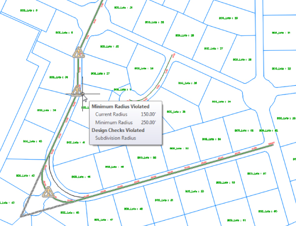
   Figure 6.28 Completed alignment layout with design criteria and design checks failure indicator

When this exercise is complete, you can close the drawing. A finished copy of this drawing is available from the book's web page with the filename 0606_AlignmentChecked_FINISHED.dwg (0606_AlignmentChecked_METRIC_FINISHED.dwg).

Now that you've created an alignment that didn't pass the design checks, let's look at different ways of modifying alignment geometry. As you correct and fix alignments that violate the assigned design checks, the warning symbols indicating those violations will disappear.

Editing Alignment Geometry

The general power of Civil 3D lies in its flexibility in design. The documentation process is tied directly to the objects involved, so making edits to those objects doesn't create hours of work in updating the documentation. With alignments, there are three major ways to edit the object's horizontal geometry without modifying the underlying construction:

1. Graphical Grip Editing Select the object and use the various grips to move critical points. This method works well for realignment, but precise editing for things such as a radius or direction can be difficult without the ability to enter values.
2. Tabular Design Use Panorama to view all the alignment segments and their properties; type in values to make changes. This approach works well for modifying lengths or radius values, but setting a tangent perpendicular to a line in the drawing or placing a control point in a specific location is better done graphically.
3. Component-Level Editing Use the Alignment Layout Parameters dialog to view the properties of an individual piece of the alignment. This method makes it easy to modify one piece of an alignment that is complicated and that consists of numerous segments, whereas picking the correct field in a Panorama view can be difficult.

In addition to these methods, you can use the Alignment Layout Tools toolbar to make edits that involve removing components or adding to the underlying component count. The following exercises look at the three simple edits and then explain how to add and remove components of an alignment without redefining it.

Grip Editing

You already used graphical editing techniques when you created alignments from polylines, but those techniques can also be used with considerably more precision than shown previously. The Alignment object has a number of grips that reveal important information about the elements' creation (see Figure 6.29).

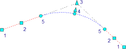
Figure 6.29 Alignment grips

You can use the grips in Figure 6.29 to do the following actions:

1. Grip 1 The square pass-through grip at the beginning of the alignment indicates a segment point that can be moved at will to change the length and angle of the line. This grip doesn't attach to any other components.
2. Grip 2 The square pass-through grip in the middle of the tangents allows the element to be moved while maintaining the length and angle. Other components attempt to hold their respective relationships, but moving the grip to a location that would break the alignment will not be allowed by the software. The change will be limited to the point where the break would occur.
3. Grip 3 The triangular grip at the intersection of tangents indicates a Point of Intersection (PI) relationship. The curve shown is a function of these two tangents and is free to move on the basis of incoming and outgoing tangents while still holding a radius.
4. Grip 4 The triangular and circular radius grips near the middle of the curve allow the user to modify the radius directly. The tangents must be maintained, so any selection that would break the alignment geometry isn't allowed.
5. Grip 5 The circular pass-through grip on the end of the curve allows the radius of the curve to be indirectly changed by changing the Point of Curvature (PC) of the alignment. You make this change by changing the curve length, which in effect changes the radius.

In the following exercise, you'll use grip edits to make one of your alignments match the planner's intent more closely:

1. Open the 0607_AlignmentEditing.dwg (0607_AlignmentEditing_METRIC.dwg) file.
2. In Prospector, expand the Alignments Centerline Alignments branch.
3. Right-click ROAD D and select Zoom To if the alignment is not within view.
4. Zoom in to the first curve of the ROAD D alignment, near station 10+00 (0+300 for metric users).

   This curve was inserted in a previous exercise using the default settings and doesn't match the guiding polyline well. If the warning symbol is in the way after zooming in, please use the regen command to update the size of the warning symbol.

5. Select the ROAD D alignment to activate the grips.
6. Select the triangular grip shown in Figure 6.30 and use a Midpoint Osnap to place it on the original polyline arc outline.

   

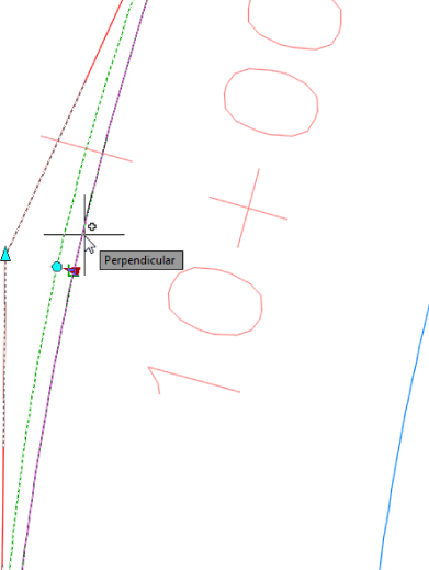
   Figure 6.30 Grip-editing the ROAD D curve

   When the triangular grip is used, the radius is changed without changing the PI.

   Keep this drawing open for the next exercise.

Your alignment of ROAD D now follows the planned layout. With no knowledge of the curve properties or other driving information, you've quickly reproduced the design's intent.

Tabular Design

When you're designing to meet jurisdictional standards, one of the most important elements is meeting curve radius requirements. It's easy to work along an alignment in a tabular view, verifying that the design meets the criteria. In this exercise, you'll verify that your curves are suitable for the design:

1. Continuing in the drawing from the previous exercise, zoom to the ROAD D alignment and select it to activate the Alignment contextual tab.
2. From the Alignment contextual tab Modify panel, choose Geometry Editor.

   You can also access the same location by selecting the alignment, right-clicking, and from the context menu selecting the Edit Alignment Geometry option.

   The Alignment Layout Tools toolbar opens.
   

3. Select the Alignment Grid View tool.

   Panorama appears as shown in Figure 6.31, with all the elements of the alignment listed along the left. You can click into many of the fields to modify their values. You can use the scroll bar along the bottom to review the properties of the alignment if necessary. Note that the columns can be resized, as well as toggled off, by right-clicking the column headers. The segment selected in the alignment grid view is also highlighted in the model, which can also make identifying the segment easier. Note that the design check failure indicators that are shown on the plan also appear in the table.

   

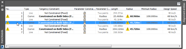
   Figure 6.31 Alignment Entities vista for ROAD D alignment

   ---

   Creating and Saving Custom Panorama Views

   If you right-click a column heading in Panorama and select the Customize Columns option at the bottom of the menu, you're presented with a Customize Columns dialog. This dialog allows you to set up any number of column views, such as Road Design or Stakeout, to show a set of different columns. These views can be saved, allowing you to switch between views easily.

   ---

4. Change the radius value of segment 4 to 400 (or 121.92 for metric users).
5. Click the close X button (notice that in the Panorama window, there is no green check mark to accept the changes) to dismiss Panorama and then close the Alignment Layout Tools toolbar.

   Keep this drawing open for the next exercise.

Panorama allows for quick and easy review of designs and for precise data entry, if required. Grip editing is commonly used to place the line and curve of an alignment in an approximate working location, but then you use the tabular view in Panorama to make the values more reasonable—for example, to change a radius of 292.56 to 300.00. Also note that for this part of the exercise, when you changed the radius, the violation for the design checks were cleared for the curve, providing feedback that you meet design requirements.

Component-Level Editing

Once an alignment gets more complicated, the tabular view in Panorama can be hard to navigate, and deciphering which element is which can be difficult. In this case, reviewing individual elements by picking them onscreen can be easier:

1. Continuing in the drawing from the previous exercise, zoom to the ROAD D alignment and select it to activate the contextual Alignment tab if not still active from the previous exercise.
2. If the Alignment Layout Tools toolbar for ROAD D is not still open from the previous exercise, from the Alignment contextual tab Modify panel, choose Geometry Editor.
   
3. Select the Sub-Entity Editor tool to open the Alignment Layout Parameters dialog for ROAD D.

   The Alignment Layout Parameters dialog opens. The dialog contents will be blank.

   Each line, arc, or spiral member of the alignment is referred to as a subentity. The Sub-Entity Editor allows you to select any segment member and edit its properties in the Alignment Layout Parameters dialog.
   

4. Select the Pick Sub-Entity tool on the Alignment Layout Tools toolbar.
5. Pick the curve that begins near station 16+00 on this alignment to display its properties in the Alignment Layout Parameters dialog (see Figure 6.32).

   

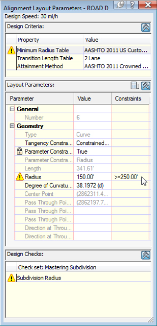
   Figure 6.32 The Alignment Layout Parameters dialog for the last curve on the ROAD D alignment

   Notice that the Tangency Constraint value currently reports Constrained On Both Sides (Free).

6. Change Parameter Constraint Lock to False.

   Notice that this will enable the ability to set many of the values that previously were grayed out and could not be set.

7. Change Parameter Constraint Lock to the original status. Change the value in the Radius field to 175 (for metric, 53.34) and watch the screen see the geometry update.

   This value is too far from the original design intent to be a valid alternative. You will reinvestigate the tangency constraints in the next exercise.

8. Change the value in the Radius field to 200 (for metric, 60.96) and again watch the update.

   This value is closer to the design and is acceptable despite being less than the minimum radius for the 30 mi/hr design speed.

9. Close the Alignment Layout Parameters dialog and the Alignment Layout Tools toolbar.

   Notice that the stationing updates.

You may keep this drawing open to continue to the next exercise or use the finished copy of this drawing available from the book's web page, 0607_AlignmentEditing_FINISHED.dwg (0607_AlignmentEditing_METRIC_FINISHED.dwg).

By using the Alignment Layout Parameters dialog, you can concisely review all the individual parameters of a component. In each of the editing methods discussed so far, you've modified the elements that were already in place. You will look at how to change the makeup of the alignment itself, not just the values driving it. But first, let's look at some of the constraints to understand how they work.

Understanding Alignment Constraints

In the previous exercise, you were exposed to constraints. The various constraints will help keep geometry together to maintain tangency or to maintain a radius.

1. A fixed segment is not constrained to its adjoining segments, so it does not maintain tangency to segments on either side.
2. A floating segment maintains tangency at one of its endpoints, but the other end is not constrained; therefore, tangency will not be maintained at the unconstrained end.
3. A free entity is constrained at both endpoints, thus maintaining tangency at both ends.

You may have noticed in Panorama the Tangency Constraint field that you looked at briefly in the previous exercise. You can click any segment and change the constraints (Figure 6.33). You can also change the constraints in the Sub-Entity Editor.

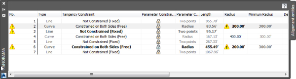
Figure 6.33 The tangency constraints in Panorama

In this exercise, you will experiment with constraints and their effect on the behavior of an alignment:

1. If your file is not still open from the previous exercise, open the 0607_AlignmentEditing_FINISHED.dwg (0607_AlignmentEditing_METRIC_FINISHED.dwg) file.
2. Select the ROAD D alignment to activate the Alignment contextual tab.
3. From the Alignment contextual tab Modify panel, choose Geometry Editor.
4. In the Alignment Layout Tools toolbar, select Alignment Grid View.
5. Click in the Tangency Constraint field for the third curve and change it to Not Constrained (Fixed).

   Notice that when you change the third curve from Constrained On Both Sides (Free) to Not Constrained (Fixed), the segment before the curve changes from Not Constrained (Fixed) to Constrained By Next (Floating).

6. Click the alignment to grip-edit the curve using the circular grip on the midpoint of the curve.

   Notice how the curve radius increases to account for the change (Figure 6.34). Also notice that the tangents are also changing to account for the change.

   

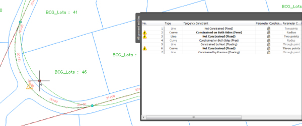
   Figure 6.34 Gripping an alignment with the tangent before the curve set to Constrained By Next (Floating) and the curve set to Not Constrained (Fixed)

   You may need to move Panorama out of the way to do this, but don't close it yet.

7. Press Esc on your keyboard to cancel the grip edit. If you inadvertently moved the curve, you can use the Undo command.
8. In Panorama, click in the Tangency Constraint field for the same curve and change it to Constrained By Previous (Floating).

   The line before the curve segment will change back to Not Constrained (Fixed).

9. Click the alignment to grip-edit the curve again using the same midpoint grip.

   Notice how the curve changes its radius but the first line maintains its bearing, while the following segment since it is floating adjusts to the new radius (Figure 6.35).

   

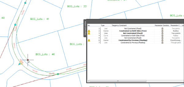
   Figure 6.35 Gripping an alignment with the tangent before the curve set to Not Constrained (Fixed) and the curve using Constrained By Previous (Floating)

10. Press Esc on your keyboard to cancel the grip edit. If you inadvertently moved the curve, you can use the Undo command.
11. Click in the Tangency Constraint field for the same curve and change it to Constrained By Next (Floating).

    The lines before it and after it will change to Not Constrained (Fixed).

12. Click the alignment to grip-edit the curve using the midpoint grip.

    Notice that the curve now maintains its tangency with the following line but not the previous line (Figure 6.36).

    

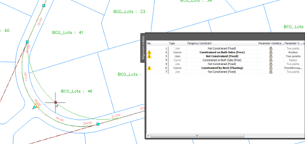
    Figure 6.36 Gripping an alignment with the curve set to Constrained By Next (Floating) and the following line set to Not Constrained (Fixed)

13. Press Esc on your keyboard to cancel the grip-edit action. If you inadvertently moved the curve, you can use the Undo command.
14. Click in the Tangency Constraint field for the third curve of the alignment and change it to Constrained On Both Sides (Free).
15. Grip-edit the curve using the same midpoint grip. See that the curve maintains its tangency with both the previous and following lines (see Figure 6.37).

    

    Figure 6.37 Gripping an alignment with the third curve on the alignment set to Constrained On Both Sides (Free) with both adjoining lines set to Not Constrained (Fixed)

16. Press Esc on your keyboard to cancel the grip edit. If you inadvertently moved the curve, you can use the Undo command.
17. Close the Alignment Layout Tools toolbar.

    When you access the Alignment Properties dialog representing an alignment containing curves, some additional options become available that were not available when the alignment was originally created. In the Point Of Intersection tab, you can select whether you want to visually show points of intersection by a change in alignment direction or by individual curves and curve groups. You can also choose to not display any implied points of intersection (see Figure 6.38).

    

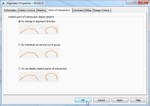
    Figure 6.38 The Point Of Intersection tab

    In the Constraint Editing tab, you can select if you want to always perform any implied tangency constraint swapping and whether to lock all parameter constraints (Figure 6.39).

    

    Figure 6.39 The Constraint Editing tab

Changing Alignment Components

One of the most common changes is adding a curve where there was none before or changing the makeup of the curves and tangents already in place on an alignment. Other design changes can include swapping out curves for tangents or adding a second curve to smooth a transition area.

As it turns out, your perfect reverse curve isn't allowed by the current ordinances for subdivision design! In this example, you'll go back to the design and place a minimum-length tangent between the curves:

1. Open the 0608_AlignmentComponents.dwg (0608_AlignmentComponents_METRIC.dwg) file.
2. Select the alignment named Reverse-Compound to activate the Alignment contextual tab.
3. From the Alignment contextual tab Modify panel, choose Geometry Editor.

   The Alignment Layout Tools toolbar appears.
   

4. Select the Delete Sub-Entity tool.
5. When prompted to select a subentity, pick the curve (C2) along alignment to remove it and press ↲ to end the command.

   Note that even if the last two curves and tangents are still part of the alignment, they lost the connection to the first part of the alignment.

6. Select the Floating Line (From Curve End, Length) option.
7. At the Select Entity to Attach to: prompt, click the south end of curve 3 and then specify a length of 100 ↲ (for metric, 30.48 ↲).
8. Select the Free Curve Fillet (Between Two Entities, Through Point) option.
9. Select the first curve (C1) segment to the west and then the line just drawn.
10. For the through point, use an Endpoint Osnap to select the free end of the tangent line just drawn and press ↲ to end the command. Notice how the stationing is now shown the full length of the completed alignment.
11. Close the Alignment Layout Tools toolbar.

    Your reverse curve with tangent section is complete, as shown in Figure 6.40.

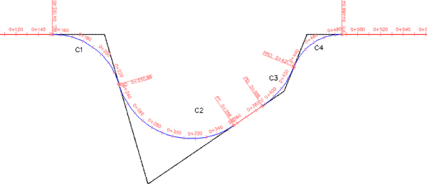
Figure 6.40 Reverse curve with tangent segment

When this exercise is complete, you can close the drawing. A finished copy of this drawing is available from the book's web page with the filename 0608_AlignmentComponents_FINISHED.dwg (0608_AlignmentComponents_METRIC_FINISHED.dwg).

So far in this chapter, you've created and modified the horizontal alignments, adjusted them onscreen according to the planners initial layout, and tweaked the design using a number of different methods. Now let's look beyond the lines and arcs and get into the design properties of the alignment.

Alignments as Objects

Alignments can represent things such as highways. Such items have design properties that help define them, and many of these design properties can be built into your Alignment properties. In addition to obvious properties such as names and descriptions, you can include functionality such as superelevation, station equations, reference points, and station control. The following sections will look at other properties that can be associated with an alignment and how to edit them.

Alignment Properties

While the properties of the alignment were originally assigned during creation, later in design there are often changes that are required. In this exercise, you'll learn an easy way to change the object style and how to add a description.

Most of an alignment's basic properties can be modified in Prospector. In this exercise, you'll change the name in a couple of ways:

1. Open the 0609_AlignmentProperties.dwg (0609_AlignmentProperties_METRIC.dwg) file and make sure Toolspace is open.
2. In Prospector, expand the Alignments Centerline Alignments branch.

   Notice that a series of alignments are listed as members.

3. Select the Centerline Alignments branch, and the individual alignments appear in the Item View (see Figure 6.41).

   

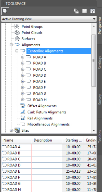
   Figure 6.41 The Alignments branch listed in the Item View of Prospector

4. Down in the Item View, click in the Name field for ROAD A and pause briefly before clicking again.

   The text highlights for editing.

5. Click in the Description field for ROAD A and enter a description (such as West-East). Press ↲.
6. Click in the Style field for ROAD A (you may have to scroll left/right to find the Style field), pause briefly, and click again; the Select Label Style dialog appears.
7. Select Basic from the drop-down menu and click OK.

   The screen updates. Keep this drawing open for the next portion of the exercise.

   That's one method to change Alignment properties. The next is to use the Properties palette.

8. Open the Properties palette by using the Ctrl+1 keyboard shortcut or some other method.
9. Select the ROAD B alignment in the drawing using the Prospector's Select option that is available when you right-click the object's name.

   The Properties palette looks like Figure 6.42.

   

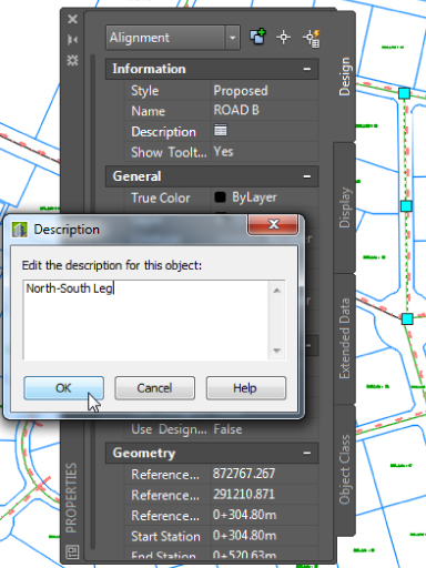
   Figure 6.42 ROAD B in the Properties palette

10. Click in the Description field, and the Description dialog will open. Enter a description (such as North-South Leg) and click OK, as shown in Figure 6.42.
11. Press Esc on your keyboard to deselect all objects and close the Properties palette if you'd like.

    Keep this drawing open for the next portion of the exercise.

    The final method involves getting into the Alignment Properties dialog, which is your access point to information beyond the basics.

12. In Prospector, right-click ROAD H and select Properties. This is the alignment for the south cul-de-sac.

    The Alignment Properties dialog for ROAD H opens.

13. Change to the Information tab if it isn't selected.
14. Enter a description in the Description field (such as South Cul-De-Sac).
15. Set Object Style to Existing.
16. Click the Apply button.

    Notice that the display style in the drawing updates immediately.

17. Click OK to accept the settings in the dialog.

    Keep this drawing open for the next portion of the exercise.

    Now that you've updated your alignments, you can make them all the same style for ease of viewing. The best way to do this is in the Prospector Item view.

18. In Prospector, expand the Alignments Centerline Alignments branch.
19. Select one of the alignments in the Item View.
20. Press Ctrl+A to select them all, or pick the top and then Shift+click the bottom item.

    The idea is to pick all of the alignments.

21. Right-click the Style column header and select Edit (see Figure 6.43).

    

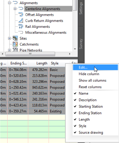
    Figure 6.43 Editing alignment styles en masse via Prospector

22. Select Layout from the drop-down list in the Select Label Style dialog that appears and click OK.
23. Press Esc to deselect all of the alignments.

    Notice that all alignments pick up this style. Although the dialog is named Edit Label Style, you are actually assigning styles to the objects.

---

Don't Forget This Technique

This technique of selecting all, right-clicking the column heading, selecting Edit, and modifying the value works on every object that displays in the Toolspace Item View, including parcels, pipes, corridors, assemblies, and so on. It can be painfully tedious to change a large number of objects from one style to another using any other method. If you left-click the column header instead of right-click, the alignments will sort alphabetically based on the values in that column.

---

You can save the drawing and if needed compare your results against the finished file that can be downloaded from the book's web page under the filename 0609_AlignmentProperties_FINISHED.dwg (0609_AlignmentProperties_METRIC_FINISHED.dwg).

Let's look at some other properties you can modify and update.

The Right Station

Every alignment has stationing applied to help locate design geometry points. This stationing may start at zero or may start at a predefined value based on previous construction. Stationing can also be fixed in both directions, requiring station equations that help translate between two disparate points that are the basis for the stationing in the drawing.

Sometimes alignments can be drawn initially in the wrong direction. Thankfully, Civil 3D has a command to fix that:

1. Open the 0610_AlignmentStations.dwg (0610_AlignmentStations_METRIC.dwg) file and make sure Toolspace is open.
2. Since the ROAD D alignment does not have the alignment labels running from north to south, you will want to reverse its direction, so pick it to activate the Alignment contextual tab.
   
3. From the Alignment contextual tab Modify drop-down panel, choose Reverse Direction.

   A warning dialog appears, reminding you of the consequences of such a change.

4. Click OK to dismiss the warning dialog.

   The stationing reverses, with 10+00 (or 0+304.80 for metric users) now at the north endpoint of the alignment.

   The warning message lets you know that when the direction is reversed, things happen to the settings defined for the alignment. Take note of what can change when an alignment is reversed. For example, if you had masking applied to the alignment, you would need to redefine it.

5. Press Esc to deselect the alignment.

   Keep this drawing open for the next portion of the exercise.

   This technique allows you to reverse an alignment almost instantly. The warning that appears is critical, though! When an alignment is reversed, the information that was derived from its original direction may not translate correctly, if at all. One prime example of this would be design profiles: they don't reverse themselves when the alignment is reversed, and this can lead to serious design issues if you aren't paying attention.

   Beyond reversing, it's common for alignments to not start with zero. For example, the ROAD E alignment may be a continuation of an existing street, and it makes sense to make the starting station for this alignment the station where this alignment intersects ROAD A, the alignment from the existing street. In this next portion of the exercise, you'll set the beginning station.

6. Select the ROAD E alignment to activate the Alignment contextual tab.
7. From the Alignment contextual tab Modify panel, choose Alignment Properties icon.
8. Switch to the Station Control tab of the Alignment Properties dialog.

   This tab controls the base stationing and lets you create station equations.

9. In the Reference Point section of the dialog, enter 2563.13 (for metric, 781.24) in the Station field (see Figure 6.44).

   

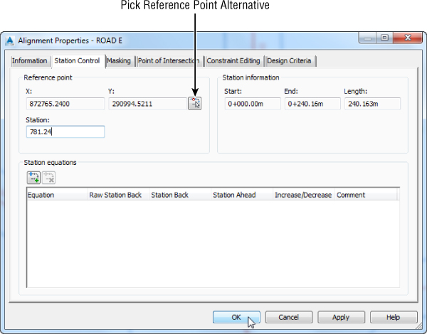
   Figure 6.44 Setting a new starting station on the ROAD E alignment

10. Click OK to dismiss the warning message that appears and click OK to dismiss the dialog.
11. Press Esc to deselect the alignment.

    The Station Information section in the top right will update. These options can't be edited but provide a convenient way for you to review the alignment's Length and Station values.

    Keep this drawing open for the next portion of the exercise.

    In addition to changing the value for the start of the alignment, you could use the Pick Reference Point button, as shown in Figure 6.44, to select another point as the stationing reference point.

    Station equations can occur multiple times along an alignment. They typically come into play when plans must match existing conditions or when the stationing has to match other plans, but the lengths in the new alignment would make that impossible without some translation. In this last portion of the exercise, you'll add a station equation on ROAD C at the intersection with ROAD B.

12. Select the ROAD C alignment to activate the Alignment contextual tab.
13. From the Alignment contextual tab Modify panel, choose the Alignment Properties icon.
    
14. On the Station Control tab of the Alignment Properties dialog, click the Add Station Equation button. You will get a warning notification. Click OK to go to the next step.
15. Use an Endpoint Osnap to select the intersection of the two alignments.
16. Change the Station Ahead value to 1000 (for metric, 304.8). You will get a warning notification. Click OK to go to the next step.
17. Click the Apply button and notice the change in the Station Information section, as shown in Figure 6.45.

    

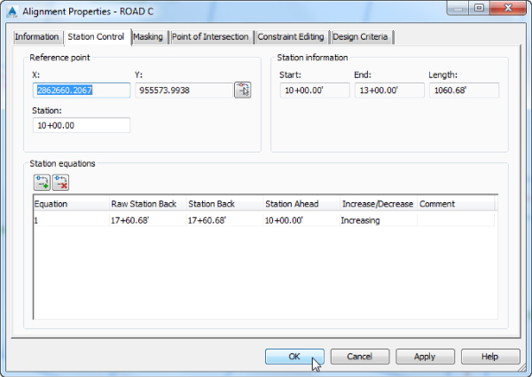
    Figure 6.45 ROAD C station equation in place

18. Click OK to accept the settings in the dialog and review the stationing that has been applied to the alignment.

You can save the drawing and if needed compare your results against the finished file that can be downloaded from the book's web page under the filename 0610_AlignmentStations_FINISHED.dwg (0610_AlignmentStations_METRIC_FINISHED.dwg).

Stationing constantly changes as alignments are modified during the initial stages of a development or as late design changes are applied to the plans. With the flexibility shown here, you can reduce the time you spend dealing with minor changes that seem to ripple across an entire project.

Assigning Design Speeds

One driving part of transportation design is the design speed. Civil 3D considers the design speed a property of the alignment, and it can be used in labels or calculations as needed. In this exercise, you'll add a series of design speeds to ROAD D. Later in the chapter, you'll label these sections of the road using a label set:

1. Open the 0611_AlignmentDesignSpeed.dwg (0611_AlignmentDesignSpeed_METRIC.dwg) file.
2. Bring up the Alignment Properties dialog for ROAD D.
3. Switch to the Design Criteria tab.
4. Verify that the Design Speed field for Number 1 is 30 mi/hr (or 48 km/hr for metric users).

   This speed is typical for a subdivision street.
   

5. Click the Add Design Speed button.
6. Click to select row 2 and then click in the Start Station.

   A small Pick On Screen button appears to the right of the Start Station value, as shown in Figure 6.46.

   

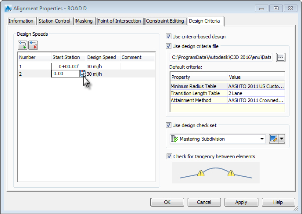
   Figure 6.46 Setting the design speed for a Start Station field

7. Click the Pick On Screen button and then use an Osnap to pick the PC on the west portion of the site, near station 9+65.78 (or station 0+294.37 for metric users)
8. Enter a value of 20 (for metric, 32) in the Design Speed field for the line you just added.
9. Click the Add Design Speed button again.

   Notice that the additional row is added to the top of the list.

10. Select the new row. Then click in the Start Station field for the new row and enter 2050 ↲ (for metric, 620.10 ↲).

    Notice that the rows reorder according to the station values in the Start Station column.

11. Enter a value of 30 (for metric, 48) for this design speed.

    When complete, the tab should look like Figure 6.47.
    

    

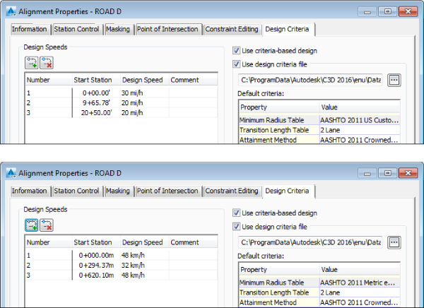
    Figure 6.47 The design speeds assigned to ROAD D alignment with both U.S. (top) and metric (bottom) values

12. Click OK to accept the settings in the Alignment Properties dialog.

You can save the drawing and if needed compare your results against the finished file that can be downloaded from the book's web page under the filename 0611_AlignmentDesignSpeed_FINISHED.dwg (0611_AlignmentDesignSpeed_METRIC_FINISHED.dwg).

In a subdivision, these values can be inserted for labeling purposes. In a highway design, they can be used to drive the superelevation calculations that are critical to a working design. Chapter 11, “Superelevation,” looks at this subject.

Labeling Alignments

Labeling in Civil 3D is one of the program's strengths, but it's also an easy place to get lost. There are many options for different labeling situations, and keeping them straight can be difficult.

The Power of Label Sets

When you think about it, any number of items can be labeled on an alignment. These include major and minor stations, geometry points, design speeds, and profile information. Each of these objects will have its own style. Applying all of these individual labeling styles one after the other would be tedious, so Civil 3D has provided you with label sets.

A label set can contain many different types of alignment labels. These sets are available during the creation and labeling process, making the application of many different types of labels less burdensome. Out of the box, a number of sets are available, primarily designed for combinations of major and minor station styles along with geometry information.

You'll learn how to create individual label styles in Chapter 18. You will use the out-of-the-box styles and label sets over the next couple of exercises.

1. Major Station Major station labels typically include a tick mark and a station callout, while the minor station labels include a tick mark only.
2. Geometry Points Geometry points refers to the PC, PT, and other points along the alignment that define the geometric properties.

In this exercise, you'll apply a label set to all of your alignments and then see how an individual label can be changed from the set:

1. Open the 0612_AlignmentLabelSets.dwg (0612_AlignmentLabelSets_METRIC.dwg) file.
2. Select the ROAD D alignment on the screen.
3. Right-click to open the context menu for the object and select Edit Alignment Labels to display the Alignment Labels dialog shown in Figure 6.48.

   

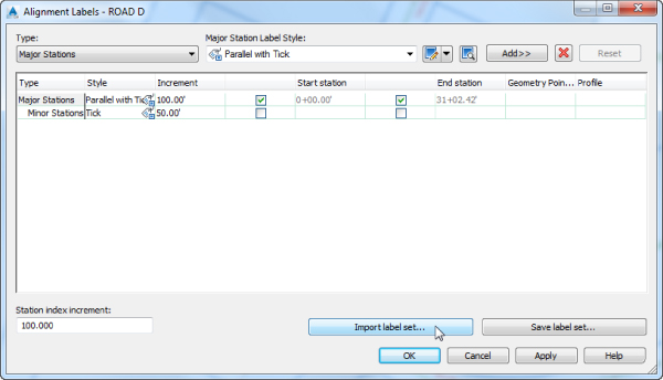
   Figure 6.48 The Alignment Labels dialog for ROAD D

4. Click the Import Label Set button near the bottom of this dialog to display the Select Label Set dialog.
5. In the Select Label Set drop-down list, select All Labels and click OK.

   The Alignment Labels dialog now populates with the additional labels imported from the label set, as shown in Figure 6.49.

   

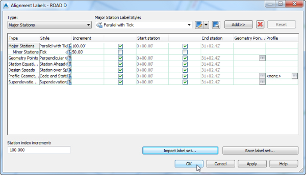
   Figure 6.49 The All Labels label set

6. Click OK to accept the settings in the Alignment Labels dialog.
7. Deselect the alignment by pressing the Esc key and repeat this process to import the All Labels set for the other alignment in the drawing.
8. When you've finished, zoom in on any of the major station labels (for example, on ROAD G, the 1+00 label, or the 0+020 label for metric users). Open the AutoCAD Properties palette using the Ctrl+1 shortcut key.
9. Select the label and notice how all of the label set group labels are selected. Notice also the properties for this group, as displayed in the AutoCAD Properties palette.
10. Press Esc to deselect.
11. Hold down the Ctrl key and select the label.

    Notice that a single label is selected, not the label set group, and the Labels contextual tab is activated.

    ---

    Ctrl+Click? What's That About?

    Prior to AutoCAD Civil 3D 2008, clicking an individual label picked the label and the alignment. Because labels are part of a label set object now, Ctrl+click is the only way to edit an individual label in a label set.

    ---

12. With the individual major station selected, in the Properties palette you will see the properties for that individual label.
13. Use the Major Station Label Style drop-down list to change from <default> to Perpendicular With Line.
14. Change the Flipped Label value to True to move the label from the left side of the alignment to the right side.

    This command can be helpful if your plans become busy and you need to move a label to the other side for better visibility.

15. Close the Properties palette and press Esc to deselect the label item.

    Keep this drawing open for the next exercise.

By using alignment label sets, you'll find it easy to standardize the appearance of labeling and stationing across alignments. Building label sets can take some time if you take into account building the label styles also, but it's one of the easiest, most effective ways to enforce standards. Building label sets will be discussed further in Chapter 18.

Station Offset Labeling

Beyond labeling an alignment's basic stationing and geometry points, you may want to label points of interest in reference to the alignment. Station offset labeling is designed to do just that. In addition to labeling the alignment's properties, you can include references to other object types in your station offset labels. The objects available for referencing are as follows:

• Alignments
• COGO points
• Parcels
• Profiles
• Surfaces
• Survey figures

In this last portion of this exercise, you'll use an alignment reference to create a label suitable for labeling the station information for the center point of the cul-de-sac along ROAD D.

1. Using the drawing from the previous exercise, from the Annotate tab Labels & Tables panel Add Labels drop-down, choose Alignment Add Alignment Labels. The Add Labels dialog appears with Feature set to Alignment.
2. In the Label Type drop-down list, select Station Offset – Fixed Point.

   The Station Offset label type creates a label that floats with the alignment. If the alignment is edited graphically, the label will move with it, and the station and offset information that it displays will remain constant. An example of this would be a label style that acts as a matchline. The counterpart label type is Station Offset – Fixed Point. This type of label will hold its position if the alignment is modified and the station and offset information change. An example of this kind of label would be labeling of a property corner on a subdivision plat.

3. In the Station Offset Label Style drop-down, select Station And Offset.
4. Leave the Marker Style field at the default setting, but remember that you could use any of these styles, including the option to use none to mark the selected point.
5. Click the Add button.
6. At the Select Alignment: prompt, select the ROAD D alignment.
7. At the Specify station along alignment: prompt, use the Center Osnap to snap to the center of the right-of-way arc at the cul-de-sac (see Figure 6.50).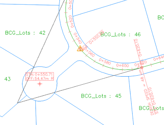

   

   Figure 6.50 The alignment station offset label in use

8. At the Specify station offset: prompt, use the Center Osnap to snap to the center of the right-of-way arc at the cul-de-sac (see Figure 6.50) again and press ↲ to end the command.
9. Close the Add Labels dialog.
10. Select the label if needed and use the square grip to drag the label to a convenient location (see Figure 6.50). Label grips will be discussed further in Chapter 18.

You can save the drawing and compare your results against the finished file that can be downloaded from the book's web page (0612_AlignmentLabelSets_FINISHED.dwg or 0612_AlignmentLabelSets_METRIC_FINISHED.dwg).

Using station offset labels and their reference object ability, you can label most site plans quickly with information that dynamically updates. Because of the flexibility of labels in terms of style, you can create design labels that are used to aid in modeling yet never plot and aren't seen in the final deliverables. More advanced alignment labels are discussed in Chapter 18.

Alignment Tables

There isn't always room to label alignment geometry along the alignment. Sometimes doing so doesn't make sense, or a reviewing agency wants to see a table showing the radius of every curve in the design. Beyond labels that can be applied directly to alignment objects, you can also create tables to meet your requirements.

You can create four types of tables:

• Line
• Curve
• Spiral
• Segment

Each of these is self-explanatory except perhaps the segment table. That table generates a mix of all the lines, curves, and spirals that make up an alignment, essentially re-creating the alignment in a tabular format. In this section, you'll generate a new line table and segment table.

All the tables work in a similar fashion. In any drawing, to add a table, follow these steps:

1. From the Annotate tab Labels & Tables panel, choose the drop-down from the Add Tables button.
2. From the Add Tables drop-down, choose the object type (such as Alignment).
3. Pick a table type (such as Add Segment) that is relevant to your work.

   The Alignment Table Creation dialog appears (see Figure 6.51).

   

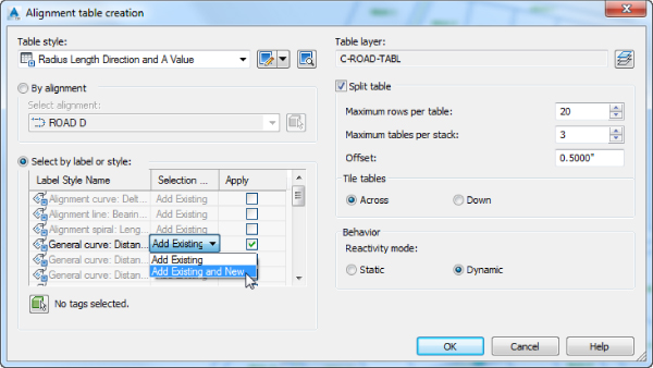
   Figure 6.51 The Alignment Table Creation dialog for the Add Segment table type

4. Select a table style from the drop-down list or create a new one.

The Select By Label Or Style area determines how the table is populated. All the label style names for the selected type of component are listed, with a check box to the right of each one. Placing a check mark in the Apply column next to one of these label styles enables the Selection Rule setting, which has the following two options:

1. Add Existing Any label using this style that currently exists in the drawing is converted to a tag format, substituting a key number such as L1 or C27, and added to the table. Any labels using this style created in the future will not be added to the table. The order in which each of the labels are converted might not be the order you desire, so you might need to renumber the label tags.
2. Add Existing And New Any label using this style that currently exists in the drawing is converted to a tag format and added to the table. In addition, any labels using this style created in the future will be added to the table.

Another way of selecting labels for an alignment table is to pick each one individually by clicking the green button under the Select By Label Or Style area.

To the right of the Select section is the Split Table section, which determines how the table is stacked up in modelspace once it's populated. You can modify these values after a table is generated, so it's often easier to leave them alone during the creation process.

Finally, the Behavior section provides two options for Reactivity Mode: Static and Dynamic. This section determines how the table reacts to changes in the labeled objects. In some cases in surveying, this disconnect is used as a safeguard to the platted data, but in general, the point of a 3D model is to have live labels that dynamically react to changes in the object. Be sure to cancel out of the Alignment Table Creation dialog before proceeding to the next exercise.

Before you draw any tables, you need to apply labels so the tables will have data to populate. In this exercise, you'll place some labels on your alignments, and then you'll move on to drawing tables:

1. Open the 0613_AlignmentTable.dwg (0613_AlignmentTable_METRIC.dwg) file.
2. From the Annotate tab Labels & Tables panel, click the Add Labels icon to open the Add Labels dialog.
3. In the Feature field, select Alignment.
4. In the Label Type field, select Multiple Segment from the drop-down list.

   With these options, you'll click each alignment one time, and every subcomponent will be labeled with the style selected here.

5. Verify that the Line Label Style field is set to Line Label Style: Bearing Over Distance (not General Line Label Style: Bearing Over Distance).

   You won't be left with these labels—you just want them for selecting elements later.

6. Verify that the Curve Label Style field is set to Delta Over Length & Radius.

   Since you have no spirals, no Spiral label style needs to be specified, so leave it at the default.

7. Click the Add button, and select each of the two alignments; then press ↲ to end the command.

   Make sure to not select the alignment multiple times during the labeling process since this will result in duplicate labels for the same segments.

8. Click the Close button to dismiss the Add Labels dialog.

   Keep this drawing open for the next exercise.

Now that you have labels to play with, let's build some tables.

Creating a Line Table

Most line tables are simple: a line tag, a bearing, and a distance. You'll also see how Civil 3D can translate units without having to change units in Drawing Settings:

1. Using the drawing from the previous exercise, from the Annotate tab Labels & Tables panel, click the Add Tables drop-down arrow and choose Alignment Add Line to open the Table Creation dialog.
2. Verify that a check mark appears in the Apply column for the Alignment Line: Bearing Over Distance label, as shown in Figure 6.52, and that the Add Existing And New rule is selected.

   

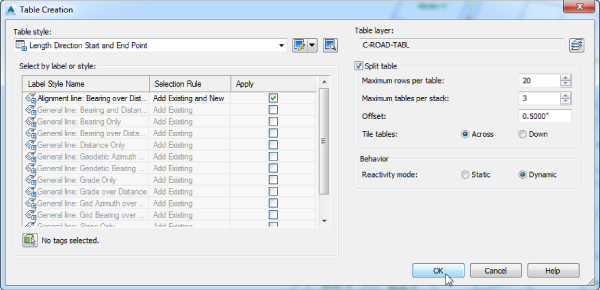
   Figure 6.52 Creating an alignment line table

3. Click OK to accept the settings in the Table Creation dialog.
4. At the Select upper left corner: prompt, select an insertion point onscreen, and the table will generate.

   Keep this drawing open for the next exercise.

You will notice that all the labels that have been selected to be displayed in the tables will have their styles modified to display the label in Tag mode. After you've made one table, creating other tables is similar. Be patient as you create tables—you must tweak a lot of values to make them look just right. By drawing one onscreen and then editing the style, you can quickly achieve the results you want.

Creating an Alignment Segment Table

An individual segment table allows a reviewer to see all the components of an alignment. In this exercise, you'll draw the segment table for ROAD D:

1. Using the drawing from the previous exercise, select the ROAD D alignment, and from the Alignment contextual tab in the Labels And Tables panel, click the Add Tables icon. From the drop-down list, choose Add Segments to open the Alignment Table Creation dialog.

   Notice that when a segment table is selected, you have the option to add the table based on the label entities assigned to an alignment, which wasn't an option when creating line and curve tables.

2. In the Select Alignment field, choose the ROAD D alignment from the drop-down list (Figure 6.53) and click OK.

   

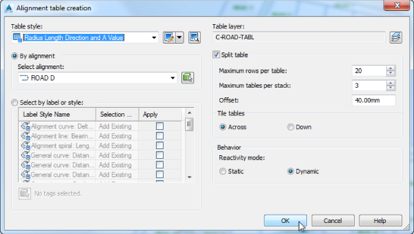
   Figure 6.53 Creating an alignment segment table

3. At the Select upper left corner: prompt, select an insertion point on the screen, and the table will generate.

When this exercise is complete, you can close the drawing. A finished copy of this drawing is available from the book's web page with the filename 0613_AlignmentTable_FINISHED.dwg (0613_AlignmentTable_METRIC_FINISHED.dwg).

The Bottom Line

1. Create an alignment from an object. Creating alignments based on polylines is a traditional method of building engineering models. With built-in tools for conversion, correction, and alignment reversal, it's easy to use the linework prepared by others to start your design model. These alignments lack the intelligence of crafted alignments, however, and you should use them sparingly.
   1. Master It Open the Masterit_0601.dwg (Masterit_0601_METRIC.dwg) file and create alignments from the linework found there, having as alignment style the Layout style, using the All Labels label set, and making sure that the source objects are erased.
2. Create a reverse curve that never loses tangency. Using the alignment layout tools, you can build intelligence into the objects you design. One of the most common errors introduced into engineering designs is curves and lines that aren't tangent, requiring expensive revisions and resubmittals. The free, floating, and fixed components can make smart alignments in a large number of combinations available to solve almost any design problem.
   1. Master It Open the Masterit_0602.dwg (Masterit_0602_METRIC.dwg) file and create an alignment using the linework on the right as a guide. Create a reverse curve with both radii equal to 200 (or 60 for metric users) and with a pass-through point at the intersection of the two arcs.
3. Replace a component of an alignment with another component type. One of the goals in using a dynamic modeling solution is to find better solutions, not just the first solution. In the layout of alignments, this can mean changing components along the design path or changing the way they're defined. The ability of Civil 3D to modify alignments' geometric construction without destroying the object or forcing a new definition lets you experiment without destroying the data already based on an alignment.
   1. Master It Convert the first curve along the alignment in the Masterit_0603.dwg (Masterit_0603_METRIC.dwg) file to a floating arc that is constrained by the next segment. Then change the radius of the curves to 150 (or 45 for metric users). Make sure that the tangency is maintained all across the alignment.
4. Create alignment tables. Sometimes there is just too much information displayed on a drawing, and to make it clearer, tables are used to show bearings and distances for lines, curves, and segments. With their dynamic nature, these tables are kept up-to-date with any changes.
   1. Master It Open the Masterit_0604.dwg (Masterit_0604_METRIC.dwg) file and generate a line table, a curve table, and a segment table. Use whichever style you want to accomplish this.