Chapter 1
The Basics
If you want to be a master in anything, you have to start with the basics. Since the Autodesk® AutoCAD® Civil 3D® platform has evolved so much over the years, now more than ever you need to have a good grip on the basics. Like with every new release of the product, manyfeatures have been enhanced, while other new ones have been added.
To get familiar with the software, you will need to go through many dialogs, ribbons, tabs, menus, and icons. Some of them may be familiar, while others will be new. This chapter will help you get used to both the familiar and the new. When you learn the interface of the Civil 3D environment and understand the terminology used in the book, everything becomes easier to use. So, please arm yourself with patience and take the time to understand every part of the workflow.
Let's start learning about the interface and Civil 3D–specific terminology. Toward the end of the chapter, you'll dive into the use of the Lines and Curves commands that, coupled with the use of transparent commands, offer multiple ways of drawing accurate lines and curves.
In this chapter, you will learn to:
- Find any Civil 3D object with just a few clicks.
- Modify the drawing scale and default object layers.
- Navigate the ribbon's contextual tabs.
- Create a curve tangent to the end of a line.
- Label lines and curves.
The Interface
If you are new to Civil 3D, this part of the chapter is especially for you, since this section will introduce you to the terminology used throughout this book. This release introduces a new startup interface that streamlines the design process. In previous versions, on startup Civil 3D created a new drawing based on a default template; with the 2015 release, you were presented with a Start tab. Now, 2016 does both: offers the Startup tab as well as creates a drawing based on the default template. Within the Start tab, four options are present: Learn, Get Started, Recent Documents, and Connect, as shown in Figure 1.1.

Figure 1.1 The Startup tab provides a quick way to get your design going.
- Learn The Learn option will take you to a dashboard containing videos that will familiarize you with new features and “Getting Started” basics. There will also be links to Learning Tips and Online Resources. To go back to the startup dashboard, click the Create option on the right.
- Get Started The Get Started section allows you to start a new drawing from a template that can be selected from the drop-down list or gives you the opportunity to open an existing file from a location, open a sheet set, find more industry-standard templates on the online repository, or open sample drawings that are provided through the software's installation.
- Recent Documents Recent Documents is pretty straightforward; it allows you to select and open a drawing from a list of most recently worked-on documents.
- Connect The Connect section deals with the Autodesk online experience for AutoCAD-based products. While using the software, you can sign in with your Autodesk account to take advantage of the cloud-enabled features within AutoCAD products. This section also provides a means to deliver software feedback to the development team.
The 2014 version introduced a new feature within the interface: tab-based access to all the files opened in the same working session. If you haven't experienced this feature in AutoCAD, you might be familiar with it in the latest browsers that use a tab-based display of open web pages, allowing quick access to any open web page, all in the same window. In the case of AutoCAD, this display shows the opened files. Using this feature, you can switch between the opened drawings just by clicking the desired file in the tab list. You can also switch between the opened drawings by using the old Ctrl+Tab key combination, but the tab-based file option lets you choose any drawing from the list of opened drawings without going through the whole list in the order in which the files were opened. On hovering over one of the file tabs, you will be presented with the option to switch between the Model and Layout tabs for that file. Figure 1.2 shows the new tab-based file feature. Other options related to the management of that drawing are available when you right-click the tab.
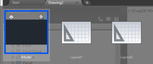
Figure 1.2 The tabbed file option allows easy switching between multiple open files and the Model and Layout tabs for the opened files.
Before we jump into the definition of the Civil 3D–specific interface items, we need to note that the overall organization of the tools and tool palettes is managed through workspaces. Once you create or open a drawing, the current workspace will be indicated on the toolbar in the top left of the application, as shown in Figure 1.3. Out of the box, the default workspace is set to Civil 3D.
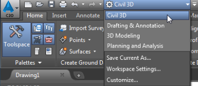
Figure 1.3 The workspace selection lets you organize the tools of the interface to suit your needs.
The workspace defines the display of the available tools based on a preset understanding of which tools are necessary for the specific tasks. The Civil 3D workspace interface is tailored to display the most common tools used for civil design, while the Planning And Analysis workspace is tailored for use with geographic information system (GIS) and mapping-industry data. Two other workspaces are available that focus on the use of basic AutoCAD tools, stripping out the Civil 3D environment and leaving in place only the core AutoCAD tools. In other words, the last two available workspaces convert your environment from a civil design–based environment to a basic drafting one. Activating any of the workspaces will result in a reorganization of the tools based on the workspace's customization. You can also save the changes you make to the current workspace or customize the whole interface based on your company's preferred layout.
Civil 3D uses a ribbon-based interface consisting of tabs and panels that organize the civil design tools based on their use in workflows. If you're used to the menu-based interface of older versions of AutoCAD verticals, you can switch to it by changing the AutoCAD MENUBAR variable from the default 0 to 1. However, the use of that menu is discouraged since ribbon management of the tools is now standard in the Civil 3D environment and the menu layout may not include all the latest tools. Therefore, in this book, we will talk about the ribbon-based interface.
On the ribbon, each of the tabs and panels is associated with one or more of the major tasks in the design process. When working on the Civil 3D 2016 ribbon, the top level in the organizational chart is represented by the tabs. The default tab, which you will see upon opening any drawing and where you will spend the majority of your time, is the Home tab, shown in Figure 1.4.

Figure 1.4 The Home tab of the ribbon and the default configuration of the ribbon for drawings with no coordinate systems assigned (top) and with them assigned (bottom)
Don't hesitate to look at the other tabs to see the many tools available, noticing that the name of each tab is assigned based on the general function of the subset of tools available under it. Furthermore, each of the tabs will provide both Civil 3D environment-specific tools and basic AutoCAD tools, reinforcing the fact that Civil 3D is a vertical product that relies on AutoCAD as its engine. The following is a description of each tab and its purpose:
- Home Tab Contains the tools you use most often in Civil 3D, including the Civil 3D object-creation tools
- Insert Tab Provides the tools for both import and insertion of data into the current drawing. Here you will find the tools to link to outside databases, manage external references, and even manage point clouds, among others.
- Annotate Tab Provides the tools to annotate both AutoCAD and Civil 3D objects within the drawing. Also in this area, the drawing-specific settings for the core AutoCAD annotative tools can be managed along with the annotative scales. You will learn more about Civil 3D annotation tools in Chapter 18, “Label Styles.”
- Modify Tab Provides the modification and editing tools for both AutoCAD and Civil 3D objects; in addition, provides access to opening the contextual ribbon tabs for Civil 3D objects
- Analyze Tab Provides the tools for performing various analyses and inquiries on the existing object data. Here you will find the tools to perform, for example, hydraulic area analysis, road design analysis, surface volumes, and estimation of quantities by means of quantity takeoffs. Also in this area is the startup for various side packages that come with Civil 3D such as the Hydraflow tools.
- View Tab Provides the tools that allow you to change the way things are displayed on the screen. Here you can define multiple viewports and customize the way objects are displayed, for example.
- Manage Tab Provides the tools for referencing data across multiple drawings via data shortcuts. Also included in this area you will find the tools to define macros, customize the user interface file, load custom runtime files, and enforce CAD standards as well as the means to import Civil 3D styles and even purge unneeded styles from the current drawing. New in 2016 will be the data shortcut manager found in this tab.
- Output Tab Provides for the production of plan sets, management of plotting, and export of data from Civil 3D to other Autodesk-based and third-party software platforms
- Survey Tab Provides the tools to manage Civil 3D survey databases. You will learn all about using and managing them in Chapter 2, “Survey.”
- Autodesk 360 Tab Provides access to the cloud services managed by the Autodesk 360 platform
- Help Tab Provides access to help tools using multiple resources
- Express Tools Tab Provides access to lots of useful AutoCAD sets of tools that have been part of the AutoCAD platform for many years
- BIM 360 Tab Provides access project collaboration tools in the BIM 360 Glue cloud
- Performance Tab Provides tools for sending performance-based reports to the AutoCAD engineering team that include detailed information about what is occurring when problems are encountered
- Geolocation Tab Provides access to the geolocation tools that were introduced in the 2014 release of the software. This is a contextual tab that is added to the list of tabs whenever a coordinate system is assigned to the drawing file.
When a Civil 3D object is selected, you will see a contextual tab appearing in the ribbon as an extension to the default group of tabs.
While these are the default tabs found in Civil 3D, their number and description can vary based on the installed add-ons and/or the user interface customization.
Please note that you can enlarge the screen area by setting the ribbon to one of its minimization states. You can access these states from the drop-down options menu located at the top-right end of the ribbon tabs, as indicated by Figure 1.5.
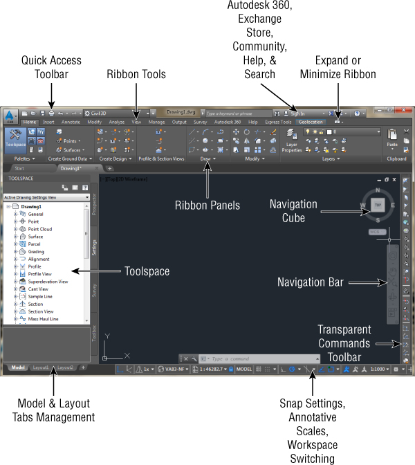
Figure 1.5 Overview of a Civil 3D environment. Toolspace is docked to the left, and the Tool Palettes panel floats over the drawing window. The ribbon is at the top of the workspace with the Quick Access toolbar above it.
Figure 1.5 shows the typical Civil 3D work environment. Besides the ribbon, you see the Quick Access toolbar, Toolspace, the Tool Palettes panel, and the Transparent Commands toolbar, among others.
On a side note, the Quick Access toolbar highlighted in Figure 1.5 gives you access to often-used tools. By default, it includes the QNew command, which creates new drawings from the default template set in Options; it also includes the Open, QSave, Print, Undo, and Redo commands. On the Quick Access toolbar, you'll also find the workspaces drop-down menu. You can add commands to this menu by clicking the drop-down to the right of the toolbar and selecting the desired command. You can also right-click an icon on the ribbon and choose Add To Quick Access Toolbar.
The ribbon is organized by tabs. Each tab is organized by panels delineated by vertical lines to the right and the left and the panel name in the bottom area. The Palettes panel on the Home tab (shown in Figure 1.6) is where you can toggle on or off different palettes. A palette is active or visible when its corresponding icon is highlighted in blue. Some of these icons enable the display of Toolspace palette tabs, while others enable the display of specific palettes.
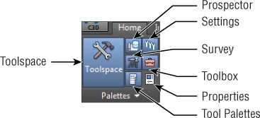
Figure 1.6 Palettes panel of the Home tab. The icons are blue when the palettes are active.
Some panels can be expanded to show additional tools. For example, in Figure 1.7, notice that on the Home tab, the Create Design panel has a drop-down arrow; if you click it, the panel will expand, and additional tools are displayed. Also, when the panels are expanded, you have the option to lock the expansion in place by toggling the pin on the bottom-left side of the expanded panel.
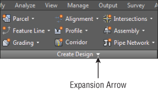
Figure 1.7 Some panels have additional tools that can be displayed by expanding the panel.
This expanded view will be locked as long as the ribbon tab is not switched. On switching to another tab, the expanded panel will minimize to the default view. You can also drag a panel out of the ribbon. It will still be visible even if the ribbon changes. You can then hover and click the icon in the upper left of the floating panel to return the panel to the original ribbon tab. There's also a button there for toggling the orientation of the floating panel.
Toolspace
Toolspace defines a set of palettes that is specific to Civil 3D. We recommend that you have this set visible anytime you are working in the Civil 3D environment. If you do not see it, click the Toolspace button on the Palettes panel of the Home tab of the ribbon.
Toolspace has four tabs to manage drawing and user data, as follows:
- Prospector
- Settings
- Survey
- Toolbox
You can turn these tabs on or off by toggling the corresponding button on the Palettes panel, but it is perfectly fine to have all four displayed at all times.
Although each tab has a unique role to play in working with Civil 3D, the Prospector and Settings tabs will be your most frequently used tabs. Survey and Toolbox serve their specific purposes, which we will examine in the following sections.
Prospector
Prospector allows you to explore your drawing file for Civil 3D objects, which makes assessing object data contained in a drawing a lot easier. Any objects will be listed under their corresponding object branch. When an object branch is expanded by clicking the plus sign to its left, Civil 3D named objects of that type are listed within the branch. Some branches, such as alignments, display object type branches when expanded. You can then expand the type branch to display the named objects of that type.
The Points branch is actually referred to as a collection. It does not expand, but it contains objects that can be displayed in Panorama. We will discuss Panorama later in this chapter. At the top of Prospector, you will see a pull-down menu giving you the following options: Active Drawing View and Master View.
Active Drawing View displays the following branches:
- The current drawing
- Data Shortcuts
Master View displays the following branches:
- All Open Drawings
- Data Shortcuts
- Drawing Templates
Master View displays every drawing you have open in the active session. The name of the active drawing you are working with appears at the top of the list in bold. To make another open drawing current, just right-click its name in Prospector and select Switch To.
In Master View, the Drawing Templates branch will contain templates saved in the path defined in Options ![]() Files tab
Files tab ![]() Template Settings
Template Settings ![]() Drawing Template File Location. You may open a template or create a new drawing with a template by right-clicking it and choosing either option from the right-click menu.
Drawing Template File Location. You may open a template or create a new drawing with a template by right-clicking it and choosing either option from the right-click menu.
Besides the two view options, Prospector has a series of icons across the top that toggle various settings on and off. Let's take a closer look at those icons:
- Item Preview Toggle This icon enables an object's graphic preview at the bottom of Prospector when Show Preview is enabled for the object category.

- Refresh Icon When Master view is enabled, the Refresh icon will display. The Refresh icon is operational only when in the Autodesk Vault Environment. Clicking it will refresh the status icons for the Vault project.

- Preview Area Display Toggle This icon will be active only when Toolspace is undocked. This button moves the preview area from the bottom of the tree view to the right of the tree view area.

- Panorama Display Toggle This icon provides one of several ways to turn on and off the display of the Panorama window. The icon will be grayed out if there are no active warnings or if you have not yet viewed data in the Panorama window.

You can always return to the Panorama window, regardless of your warning status, by clicking the Event Viewer button from the Home tab
 Palettes panel.
 - Help Don't underestimate how helpful Help can be!

The Data Shortcuts branch provides access to shared Civil 3D objects across the project, which are objects that can be referenced into the current drawing and updated dynamically from their source (you will learn about data shortcuts and how to work with and manage them in Chapter 16, “Advanced Workflows”). Each main grouping under the drawing name is referred to as a branch. If you expand a branch by clicking the plus sign next to its name, you will see the contents of that branch. Also, you will notice that some of the branches are subcategorized based on their functional class. For example, by expanding the Alignments group, you will notice the functional subdivision based on the purpose for that object. In the case of the alignments, this categorization is assigned on object creation but can be changed at any time in the Alignment Properties dialog. You will learn about this in Chapter 6, “Alignments.”
Because all Civil 3D data is dynamically linked, you will see object dependencies as well. You can learn details about an individual object by expanding its group type collection and selecting the object (Figure 1.8).
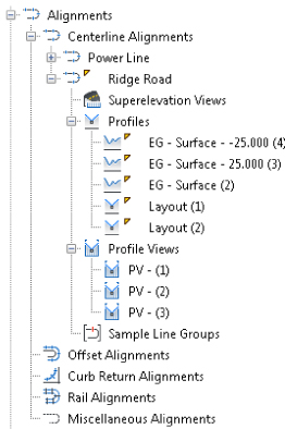
Figure 1.8 A look at the Alignments group branch of the Prospector tab. Profiles and Profile Views are linked to alignments; therefore, they appear under Alignments.
When an object branch is selected, the bottom of Prospector displays the Item View. Clicking the plus sign next to the object branch also provides you with the list of the objects created under that object type. Using the Item View, you can edit the object's name, description, and style without having to open the Civil 3D Properties dialog. Right-clicking the object type gives you access to a number of commands that apply to all the members of that collection. For example, right-clicking the Point Groups branch brings up the menu shown in Figure 1.9 (left).
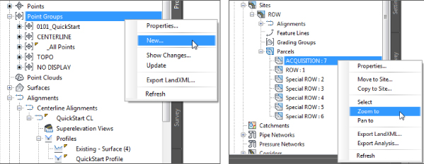
Figure 1.9 Context-sensitive menus in Prospector for creating new objects (left) and zooming to a specific object (right)
In addition, right-clicking the individual object offers many commands unique to Civil 3D, such as Zoom To and Pan To, shown in Figure 1.9 (right). By using these commands, you can find any parcel, point, cross section, or other Civil 3D object in your drawing almost instantly.
For example, if you are interested in locating a parcel named ACQUISITION : 7 using the Zoom To command, locate the Sites branch on the Prospector tab of Toolspace. Expand Proposed Site and highlight Parcels. Select the Parcel object either from the Item View or from the expanded Parcels collection, right-click, and select Zoom To. Civil 3D will locate the object and zoom to its whereabouts.
Also, note that by using the Properties option shown under the context menu for the object (see Figure 1.10, left), you can access its settings. Within the dialog that opens, you can modify the object's name, select its Civil 3D display style, and change its description, among other tasks (see Figure 1.10, right).
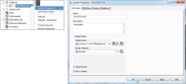
Figure 1.10 The Civil 3D object Properties dialog allows you to define the object's name, style, and definition and perform specific tasks in some cases.
As you navigate the tabs of Toolspace, you will encounter many symbols to help you along the way. Table 1.1 shows you a few that you should familiarize yourself with.
Table 1.1 Common Toolspace symbols and meanings
| Symbol | Meaning |
 |
This represents the object or style is in use. It also appears when there is a dependency to the object or if the style has child styles. For example, you will see this icon on a surface when a profile has been created from it. |
 |
Clicking this will expand the object branch of Toolspace. |
 |
Clicking this will collapse the object branch of Toolspace. |
 |
This indicates a collection. Data resides in a collection, and more information will be listed in the Item View. |
 |
The object needs to be rebuilt or updated. This can also indicate a broken data reference. |
 |
Civil 3D may still be processing the object, or the collection of Prospector needs to be refreshed. |
 |
This symbol next to an object indicates that the object is data referenced from another drawing. A larger version of this icon is shown next to the Data Shortcuts branch of the Prospector tab. |
Settings
The Settings tab of Toolspace provides the tools to manage the way Civil 3D objects display in the drawing and define the default behavior of the commands associated with the creation of these objects. Any annotation or text that is placed by Civil 3D is controlled by Label styles. Object styles control the way the features of the Civil 3D objects are displayed within the drawing. So if you take, for example, an alignment, the dynamic annotation of the stationing, offsets, and the like is controlled by its Label styles, while its graphic representation is controlled by the Object styles.
These settings and styles are defined and contained within the drawing itself; therefore, the need for a good template that defines these items before you begin working is obvious. When you have a standard defined for your Civil 3D drawings, these settings and styles will already be set so that you can go ahead and start your design. Chapters 18 and 19 are dedicated to the management and definition of these styles. Later in this chapter, you will learn more about templates.
Drawing Settings
As with the Prospector tab, at the top of the Settings tab you will see the name of the drawing. When using Civil 3D, it is a common startup practice to make sure that your drawing settings match the requirements of the project. To access the overall settings for the current drawing, from the Toolspace Settings tab, right-click its name and select Edit Drawing Settings from the displayed list, as shown in Figure 1.11, to access the Drawing Settings dialog.

Figure 1.11 Accessing the Drawing Settings dialog
Each tab in this dialog focuses on the management of specific settings for the drawing. If the settings for the Object Layers, Abbreviations, and Ambient Settings tabs are usually the same over all your projects, you can define them from a company-wide template. Because that does not usually apply for the drawing scale and coordinate information settings, which are project specific based on the desired output or its geographic location, you are likely to visit this tab at least once for each design file.
The Units And Zone Tab
On the Units And Zone tab, you have the option to define the default measurement system by selecting the default drawing units from the drop-down menu. In the same place you also have the option to define how the Imperial-to-metric conversion is handled. For the base template that ships with Civil 3D, by default the conversion takes the International Foot. If no coordinate system is assigned to the drawing, as in the case of the stock template, then by default your drawing will have assigned a No Datum, No Projection coordinate system. As soon as a coordinate system is selected from the Zone portion of the dialog, the Imperial To Metric Conversion option becomes grayed out. This happens because by assigning a coordinate system to the drawing, the coordinate system will take care of the conversion for you.
This tab also includes the options Scale Objects Inserted From Other Drawings and Set AutoCAD Variables To Match. The Set AutoCAD Variables To Match option sets the base AutoCAD angular units, linear units, block insertion units, hatch pattern, and linetype units to match the values set in this dialog. As shown in Figure 1.12, even though these settings are enabled in the figure, the base template has them disabled in order to avoid issues that might arise based on work environments. So, feel free to experiment with them and see how they affect your data.
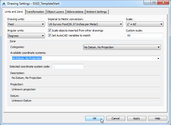
Figure 1.12 Before placing any project-specific information in a drawing, set the coordinate system in the Units And Zone tab of the Drawing Settings dialog.
The scale that you see on the right side of the Units And Zone tab is the same as your annotation scale. You can change it here, or you can change it by selecting the desired scale from the annotation scale list in the bottom-right corner of the drawing window. Note that this scale is available only in modelspace.
In the Zone area of the Units And Zone dialog, if you choose to work with the default No Datum, No Projection option, then you will work using an assumed coordinate system. However, since most projects today are developed within a spatial reference, it is advisable to set the coordinate system to the one that is local to the area of your project. If your drawing file does not require the use and management of space-referenced data, then you can leave the coordinate system set to No Datum, No Projection.
Civil 3D has an extensive database of coordinate systems that can be assigned. This database is common to and shared across multiple Autodesk products. The first step in assigning the coordinate system is to select the category that your coordinate system resides in. The categories are based on geographic location. Since Civil 3D is used worldwide, its coordinate system's database contains most of the standard coordinate systems (including the obsolete ones). Once the category is selected, the collection of coordinate systems that are available within that category will be listed in the Available Coordinate Systems drop-down.
As soon as a coordinate system is selected, you will notice that the Selected Coordinate System Code, Description, Projection, and Datum areas will be filled with the specific data that defines that coordinate system. If you use a coordinate system often, a quick way to select that system is by inputting its code in the Selected Coordinate System Code section of the dialog.
Try the following quick exercise to practice setting a drawing coordinate system:
- Open the drawing
0102_TemplateStart.dwg(0102_TemplateStart_METRIC.dwg).You can download this and all other files related to this book from this book's web page,
www.sybex.com/go/masteringcivil3d2016. - Switch from Toolspace's Prospector tab to the Settings tab.
- Right-click the filename and select Edit Drawing Settings.
- Switch to the Units And Zone tab to display the options shown previously in Figure 1.12.
- Select USA, Texas from the Categories drop-down menu on the Units And Zone tab.
- Select NAD83 Texas State Planes, Central Zone, US Foot (NAD83 Texas State Planes, Central, Meter) from the Available Coordinate Systems drop-down menu.
You could have also typed TX83-CF (TX83-C) in the Selected Coordinate System Code box.
- Click OK and save the drawing for use in an upcoming exercise.
Notice that once you have set the coordinate system, the Geolocation tab becomes active in the ribbon, and you can use the tools that are available under this tab.
By default, the mapstatusbar variable is now set to Show, which displays the name of the coordinate system on the status bar. If you do not want the coordinate system name displayed in the bottom bar, run the mapstatusbar command and change its status from the default of Show to Hide.
The Transformation Tab
Most survey-grade global positioning system (GPS) equipment takes care of the transformation to local grid coordinates for you. In the United States, state plane coordinate systems already have regional projections taken into account. In the rare case that surveyors need to manually transform local observations from geoid to ellipsoid and ellipsoid to grid, the Transformation tab enables access to enter transformation factors.
With a base coordinate system selected, you can do any further refinement you'd like using the Transformation tab, shown in Figure 1.13. The coordinate systems on the Units And Zone tab can be refined to meet local ordinances, tie in with historical data, complete a grid-to-ground transformation, or account for minor changes in coordinate system methodology.
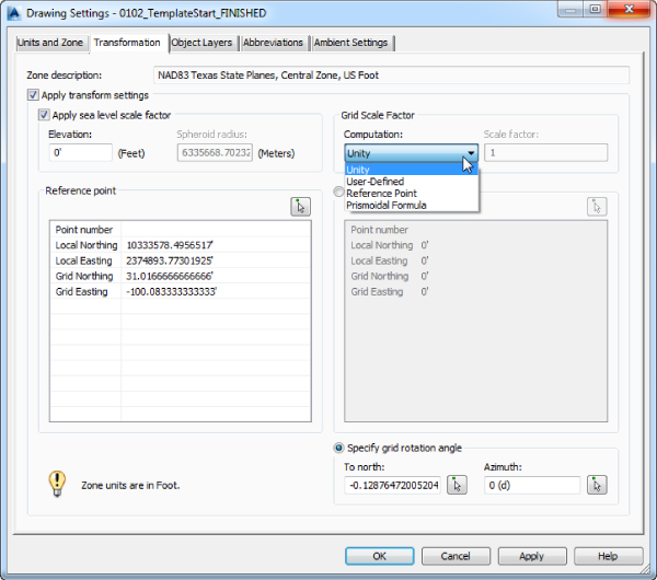
Figure 1.13 The Transformation tab
These changes can be made with the following options:
- Apply Sea Level Scale Factor This value is known in some circles as elevation factor or orthometric height scale. The sea level scale factor takes into account the mean elevation of the site and the spheroid radius that is currently being applied as a function of the selected zone ellipsoid.
- Grid Scale Factor At any given point on a projected map, there is a distortion between the “flat” measurement and the measurement on the ellipsoid. In the Grid Scale Factor area, you are presented with four options. When your selection is set to Unity, the grid factor is assumed to be 1, which basically disables the grid scale factor. In the case of User-Defined, which is the most-used option, you will provide a scale factor.
- When you use this option, the Civil 3D Northing and Easting values define the localized or project coordinates, while the Grid Northing and Grid Easting values define an approximation of the grid coordinates for the point. If you choose Reference Point, Civil 3D will determine a scale factor that is based on a selected reference point. The last option is Prismoidal Formula, where Civil 3D defines a different grid scale factor for each point in the drawing.
- Reference Point To apply the grid scale factor and the sea level factor correctly, you need to tell Civil 3D where you are on Earth. You can use Reference Point to set a transformation value for a singular point in the drawing field via the pick button or the Point Number. The pick button and point number options both populate the Local Northing and Local Easting values. The Grid Northing and Grid Easting values must be entered manually.
- Rotation Point Rotation Point can be used to set the reference point for rotation via the same methods as for the reference point. The pick button and point number options both populate the Local Northing and Local Easting values. The Grid Northing and Grid Easting values must be entered manually.
- Specify Grid Rotation Angle Some people may know this as the convergence angle. This is the angle between Grid North and True North. Enter an amount or set a line to north by picking an angle or deflection in the drawing. You can use this same method to set the azimuth if desired. You can assign a rotation point or a grid rotation angle, but not both at the same time.
It should be noted that this is not the place to transform assumed coordinates to a predefined coordinate system. See Chapter 2 to learn how to translate a survey.
The Object Layers Tab
When you think about AutoCAD, you imagine lines, polylines, circles, and so on. Civil 3D adds its own specific entities, including points, surfaces, alignments, corridors, and others. All Civil 3D objects at the basic level comprise basic-level AutoCAD entities, but Civil 3D objects are dynamic elements.
Civil 3D is built on top of AutoCAD; therefore, all the objects reside on layers. When you define a basic AutoCAD object, you know the object will be created and placed in the current layer. When Civil 3D objects are created, they are placed on a predetermined object layer set up in your Civil 3D template.
Layers are found in several areas of the Civil 3D template. The first location you will examine is the Drawing Settings dialog ![]() Object Layer tab. The layers listed here represent overall layers where the objects will be created. For those of you who are familiar with AutoCAD blocks, it is useful to think of these layers in the same way as a block's insertion layer.
Object Layer tab. The layers listed here represent overall layers where the objects will be created. For those of you who are familiar with AutoCAD blocks, it is useful to think of these layers in the same way as a block's insertion layer.
In the Object Layers tab, every Civil 3D object must have a layer set, as shown in Figure 1.14. It is a common practice to not have any of the object layers set to 0. An optional modifier can be added to the beginning (prefix) or end (suffix) of the layer name to further separate items of the same type.
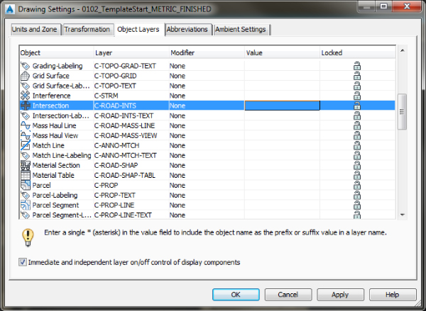
Figure 1.14 For each Civil 3D object type in the list, a placement layer is defined for the new objects.
A common practice is to add wildcard suffixes to corridor, surface, pipe, and structure layers to make it easier to manipulate them separately. For example, if the layer for a corridor is specified to be C-ROAD-CORR and a suffix of -* (dash asterisk) is added as the modifier value, a new layer will automatically be created when a new corridor is created. The resulting layer will take on the name of the corridor in place of the asterisk. If the corridor is called Congress Ave, the new layer name will be C-ROAD-CORR-Congress Ave. This new layer is created once and is not dynamically linked to the object name. In other words, if you find out that you got the name of the street wrong and need to change it, you can't just change the name of the Civil 3D object.
If the layer name that you chose to use for an object does not exist in the drawing, you can create it as you work through the Object Layers dialog. To access the mentioned dialog and be able to create a new layer if needed, double-click the layer name assigned to the object within the Layer column, and if the layer is not within the list, click the New button and set up the layer as needed, including color, lineweight, linetype, and so forth, as shown in Figure 1.15.
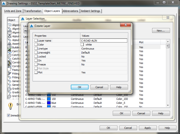
Figure 1.15 After you click New, you can set up a new layer.
Make sure you have the Immediate And Independent Layer On/Off Control Of Display Components setting checked. As mentioned earlier, the layers listed here are the ones the objects will reside on. However, even though the objects reside in those layers, their display components can be configured to other layers as defined by the Object styles, which you will learn about in Chapter 19. Having this option selected means that when you turn off the layer in which an object resides, its graphic display of its components will act independently of the object. When this option is cleared, by turning off the layer the object layer resides on, all its components will be turned off, with no regard to what layer they reside on.
In the following exercise, you will set object layers in a template:
- Continue working in the drawing that you saved in the previous exercise,
0102_TemplateStart.dwg(0102_TemplateStart_METRIC.dwg). - From the Settings tab of Toolspace, right-click the name of the drawing and select Edit Drawing Settings.
- Switch to the Object Layers tab.
- Double-click the Layer field next to Alignment and click New to create a new layer in the Layer Selection dialog box (see Figure 1.15).
- Create a new layer called C-ROAD-ALIN. Leave other layer settings at the defaults. Click OK.
- Select the newly created layer as the layer for the Alignment object in the Layer Selection dialog and click OK.
- Set the layer for Building Site to A-BLDG-SITE. Since the layer is already present in the drawing, you can just select it from the Layer Selection dialog's Layers list.
- Set the layer for Catchment-Labeling to C-HYDR-CTCH-TEXT.
- For the Corridor layer, keep the main layer as C-ROAD-CORR.
- Set the modifier to Suffix by clicking the Modifier field and selecting Suffix from the drop-down list.
- Set the modifier value to -* by clicking and typing it in the Value column field for the object.
The asterisk acts as a wildcard that will add the corridor name as part of a unique layer for each corridor, as previously described.
- Scroll down to locate the Pipe in the Object list.
- Create several new layers and add suffix information.
- For Pipe, create a layer called C-NTWK-PIPE with a modifier of Suffix and a value of -*.
- For Pipe-Labeling, create a new layer called C-NTWK-PIPE-TEXT.
- For Pipe And Structure Table, set the layer to C-NTWK-PIPE-TABL.
- For Pipe Network Section, create a new layer called C-NTWK-SECT.
- For Pipe Or Structure Profile, create a new layer called C-NTWK-PROF.
- Scroll down a bit further and create a new layer for Structure called C-NTWK-STRC.
- Add a modifier of Suffix and a value of -*.
- For Structure-Labeling, create a new layer called C-NTWK-STRC-TEXT.
- Add a modifier of Suffix to the Tin Surface object layer and a value of -*. Your layers and suffixes should now resemble Figure 1.16.

Figure 1.16 Examples of the completed layer names in the Object Layers tab
- Click to place a check mark next to Immediate And Independent Layer On/Off Control Of Display Components.
As described previously, this setting will allow you to use the On/Off toggle in the layer manager to work with Civil 3D objects.
- Click Apply and then OK.
- Save the drawings.
You can check your finished drawings against the completed file that can be downloaded from the book's web page. The file you will be looking for is 0102_TemplateStart_FINISHED.dwg (0102_TemplateStart_METRIC_FINISHED.dwg).
The Abbreviations Tab
When you add labels to certain objects, Civil 3D automatically uses the abbreviations assigned in this tab to indicate geometry features. For example, left is L, and right is R. Figure 1.17 shows a sampling of customizable abbreviations.
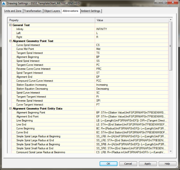
Figure 1.17 Features are customizable down to the letter on the Abbreviations tab.
Civil 3D uses industry-standard abbreviations wherever they are found. If necessary, you can easily change VPI to PVI for Point of Vertical Intersection. In most cases, changing an abbreviation is as simple as clicking in the Value field and typing a new one. You might notice that most of the abbreviations are simply defined, but some of them are defined by using macros, as in the case of the Alignment Geometry Point Entity Data. You will find that these macros are widely used in the naming conventions for the Civil 3D objects.
The Ambient Settings Tab
Examine the settings in the Ambient Settings tab to see what can be set here. The main options you'll want to adjust are in the General category, and the display precision settings are in the subsequent categories. You will also want to visit the Angle and Direction categories to verify the format of the angles.
The level of precision that you see in this dialog does not change the precision in labels. What you see here is the number of decimal places reported to you in various dialog boxes.
Becoming familiar with the way this tab works will help you further down the line because almost every other settings dialog box in the program works like the one shown in Figure 1.18.
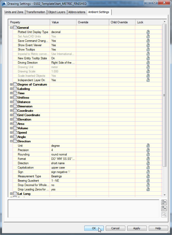
Figure 1.18 Ambient Settings at the main drawing level
You can set the following options in the General category:
- Plotted Unit Display Type Civil 3D knows you want to plot at the end of the day. In this case, it's asking how you would like your plotted units measured. For example, would you like that bit of text to have a height of 0.25” or ¼”? In the civil engineering world there is mostly a consensus on the use of decimal units. For example, many people who used Land Desktop before Civil 3D are comfortable with the Leroy method of text heights (L80, L100, L140, and so on), so the decimal option is an obvious choice.
- Set AutoCAD Units This option specifies whether Civil 3D should attempt to match AutoCAD drawing units, as specified on the Units And Zone tab. This setting is specified on the Units And Zone tab but is displayed here for reference so you can lock it if desired.
- Save Command Changes To Settings Set this to Yes. This setting is incredibly powerful but a secret to almost everyone. By setting it to Yes, you ensure that your changes to commands will be remembered from use to use. This means if you make changes to a command during use, the next time you call that Civil 3D command, you won't have to make the same changes. By setting it to Yes, you will save yourself the frustration of setting it over and over again.
- Show Event Viewer Event Viewer is the main Civil 3D feedback mechanism, especially when things go wrong. Event Viewer uses the Panorama interface to display warnings such as when a surface contains crossing breaklines. Event Viewer will pop up with informational messages as well. If you have multiple monitors, it is a good idea to leave Panorama on but set aside for review.
- Show Tooltips One of the cool features that people remark on when they first use Civil 3D is the small pop-up that displays relevant design information when the cursor is paused on the screen. If the cursor is paused over an object, it will display some basic properties about that object. If it is paused in a blank space on the screen, depending on the Civil 3D objects present in the drawing, it can provide horizontal and/or vertical data of the position of the cursor relative to those objects or within the definition area of the object. For example, for alignments it can provide name, station, and offsets of the cursor relative to all the alignments in the drawing as long as the cursor position from the alignments is perpendicular; for a surface, it can provide the name and the elevation of the point the cursor is placed over.
Once a drawing gets complex, the amount of data displayed in the tooltip can be overwhelming; therefore, Civil 3D offers the option to turn off these tooltips universally with this setting. If you want to micromanage these tooltips, then you have the option to toggle the tooltip display for each Civil 3D object individually by accessing the toggle found in the Information tab of the Properties dialog for those objects.
- Imperial To Metric Conversion This setting displays the conversion method specified on the Units And Zone tab. The two options are US Survey Foot and International Foot. This setting is specified on the Units And Zone tab but is displayed here for reference so you can lock it if desired.
- New Entity Tooltip State This setting controls whether the tooltip is turned on at the object level for new Civil 3D objects. If you change this setting to Off partway through a project, the tooltip will not be displayed for any Civil 3D objects created after the change. Of course, you can go back to each of the objects and enable the tooltip if necessary.
- Driving Direction This specifies the side of the road that forward-moving vehicles use for travel. This setting is important in terms of curb returns and intersection design.
- Drawing Unit, Drawing Scale, and Scale Inserted Objects These settings are specified on the Units And Zone tab but are displayed here for reference and so that you can lock them if desired.
- Independent Layer On This is the same control that is set on the Object Layers tab. Yes is the recommended setting, as described previously.
Moving down to the Direction category, you have the following choices:
- Unit Degree, Radian, and Grad
- Precision 0 through 8 decimal places
- Rounding Round Normal, Round Up, and Truncate
- Format Decimal, DD°MM' SS.SS", DD°MM'SS.SS" (Spaced) and DD.MMSSSS (decimal dms)
In most cases, people want to display DD°MM'SS.SS". Also, this setting controls how directions are entered at the command line.
- Direction Short Name (spaced or unspaced) and Long Name (spaced or unspaced)
- Capitalization You can preserve case or force uppercase, lowercase, or title caps.
- Sign Gives you a choice of how negative numbers are displayed. You can use a minus sign to denote negative numbers only, use a set of parentheses to denote a negative, or use a sign regardless of value. The latter option will show a plus for positive values and a minus for negative values.
- Measurement Type Bearings, North Azimuth, and South Azimuth
- Bearing Quadrant This should be left at the industry standard: 1 – NE, 2 – SE, 3 – SW, 4 – NW.

When you're using the Bearing Distance transparent command, for example, these settings control how you input your quadrant, your bearing, and the number of decimal places in your distance.
Besides the Direction category, you can explore the other categories, such as Angle, Lat Long, and Coordinate, and customize the settings to how you work.
At the bottom of the Ambient Settings tab is a Transparent Commands category. These settings control how (or if) you're prompted for the following information:
- Prompt For 3D Points Controls whether you're asked to provide a z elevation after x and y have been located
- Prompt For Y Before X For transparent commands that require x and y values, this setting controls whether you're prompted for the y-coordinate before the x-coordinate. Most users prefer this value set to False so they're prompted for an x-coordinate and then a y-coordinate.
- Prompt For Easting Then Northing For transparent commands that require Northing and Easting values, this setting controls whether you're prompted for Easting first and Northing second. Most users prefer this value set to False so they're prompted for Northing first and then Easting.
- Prompt For Longitude Then Latitude For transparent commands that require Longitude and Latitude values, this setting controls whether you're prompted for Longitude first and Latitude second. Most users prefer this value set to False so they're prompted for Latitude and then Longitude.
The settings that are applied here can be changed both at the drawing level and at the object level. For example, you may typically want elevation to be shown to two decimal places, but when looking at surface elevations, you might want just one. The Override and Child Override columns give you feedback about these types of changes (see Figure 1.19).

Figure 1.19 The Child Override indicator in the Time, Distance, and Elevation values
The Override column shows whether the current setting is overriding something higher up. Because you're at the Drawing Settings level, these are clear. However, the Child Override column displays a down arrow, indicating that one of the objects in the drawing has overridden this setting. You can check child overrides by accessing the Feature Settings of an object such as a surface (see Figure 1.20, left) and looking for a filled Override check box (see Figure 1.20, right).
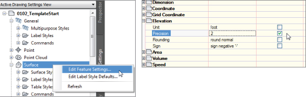
Figure 1.20 The Surface Edit Feature Settings and the Override indicator
Notice that in this dialog, the box for the Precision setting is checked in the Override column. This indicates that you're overriding the settings mentioned earlier, and it's a good alert that things have changed from the general drawing settings to this object-level setting.
But what if you don't want to allow those changes? Each settings dialog includes one more column: Lock. At any level, you can lock a setting, graying it out for lower levels. This can be handy for keeping users from changing settings at the lower level that perhaps should be changed at a drawing level, such as sign or rounding methods.
Survey
The Survey tab of Toolspace is where survey settings, equipment settings, linework code sets, and figure prefix database settings are controlled. You can toggle this tab off and on by using the corresponding button under the ribbon's Home tab ![]() Palettes panel. Surveying is an essential part of land-development projects. Because of the complex nature of this tab, all of Chapter 2 is devoted to it.
Palettes panel. Surveying is an essential part of land-development projects. Because of the complex nature of this tab, all of Chapter 2 is devoted to it.
Toolbox
The Toolbox tab of Toolspace is a launching point for add-ons and reporting functions. To display the Toolbox, from the Home tab of the ribbon, under the Palettes panel you can find the Toolbox icon to enable/disable the tab. The location of this icon was shown previously in Figure 1.6. Out of the box, the Toolbox contains reporting tools created by Autodesk, but you can expand its functionality to include your own macros or reports. The buttons on the top of the Toolbox, shown in Figure 1.21, allow you to customize the report settings and add new content. If you are an Autodesk® Subscription customer, here is where you will find lots of the add-ons released for subscription customers only.

Figure 1.21 The Toolbox with the Edit Toolbox Content icon highlighted
Panorama
The Panorama window is the Civil 3D feedback and tabular editing mechanism. It's designed to be a common interface for a number of different Civil 3D–related tasks, and you can use it, for example, to provide input in the creation of profile views, to edit pipe or structure information, or to run basic volume analysis between two surfaces. For an example of Panorama in action, open it by going to the Home tab ![]() Palettes panel flyout and clicking the Event Viewer icon. You'll explore and use Panorama more during this book's discussion of specific objects and tasks.
Palettes panel flyout and clicking the Event Viewer icon. You'll explore and use Panorama more during this book's discussion of specific objects and tasks.
Contextual Ribbon Tab
As with AutoCAD, the ribbon is the primary interface for accessing Civil 3D commands and features. When you select an AutoCAD Civil 3D object, the ribbon displays commands and features related to that object in a contextual tab. If several object types are selected, the Multiple contextual tab is displayed. Use the following procedure to familiarize yourself with the contextual tab of the ribbon:
- Open
0103_Example.dwg (0103_Example_METRIC.dwg), which you will find atwww.sybex.com/go/masteringcivil3d2016. - Select the parcel label reading Acquisition : 7.
Notice in the Parcel contextual tab that the Labels & Tables, General Tools, Modify, and Launch Pad panels are displayed, as shown in Figure 1.22.
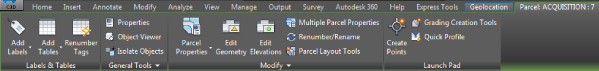
Figure 1.22 The Parcels contextual tab within the ribbon
- With the Parcel still selected, click a parcel line and notice the display of the Multiple contextual tab (Figure 1.23).
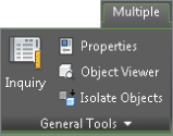
Figure 1.23 When more than one object is selected, the Multiple contextual tab appears.
- Use the Esc key to cancel all selections.
- Reselect a parcel by clicking one of the numeric labels.
- Select the down arrow next to the Modify panel name.
- Click the pin at the bottom-left corner of the panel to keep it open.
- Select the Properties command in the General Tools panel to open the AutoCAD Properties palette.
Notice that the Modify panel remains open and pinned until the current selection set changes.
Civil 3D Templates
Styles and settings should be defined within your template. Some people manage to have all the settings and styles defined within a single file, while others take the approach of separating the templates based on the type of projects they deal with. Therefore, we assume your template will have all the styles you need for the type of project you are working on. If you find you are constantly changing style settings, you should reexamine your workflow.
When starting a project or continuing a project from an outside source, it is important to start with a Civil 3D template file. You will find all the information you need on customizing the template to have the desired styles for both objects and annotations in Chapters 18 and 19.
Right after installing the software, you will see two usable Civil 3D–specific templates (Figure 1.24).

Figure 1.24 Selecting a Civil 3D template by going through the Application menu ![]() New
New ![]() Drawing
Drawing
Starting New Projects
When you start a project with the correct template file (defined by a .dwt file extension), the repetitive task of defining the basic framework for your drawing is already completed. Since Civil 3D runs on top of AutoCAD, the template will have two parts. The first part of the Civil 3D template is the AutoCAD side of the template, and it will contain the following:
- Unit type (architectural or decimal) and insertion scale (meters or feet)
- Layers and their respective linetypes, colors, and other properties
- Text, dimension, tables, and multileader styles
- Layouts and plot setups
- Block definitions
The second part is represented by the specific Civil 3D side. Therefore, in addition to the items just listed, you will encounter the following:
- More specific unit information (international feet, survey feet, or meters), together with the coordinate systems defined within the Drawing Settings dialog that you've learned about.
- Civil object layers, defined with the object layers. (You've learned about this one, as well.)
- Ambient settings. (Try to remember, did you see this one somewhere already?)
- Label styles and formulas (expressions). (There is an awesome chapter on this: Chapter 18.)
- Object styles. (Chapter 19 will give you all you need to know about them.)
- Command settings of which you'll learn more in this chapter. (The customization takes a new level when these are defined.)
- Object-naming templates defined by macros within command settings. (Your typing life will be so much easier when these are defined.)
- Report settings that can be found within the Toolbox tab of Toolspace.
- Description key sets. (You will learn how these can streamline your survey processing in Chapter 2.)
Now that you've learned what makes up the Civil 3D template, make sure to start your design adventure using the proper template. Many times you will receive files from people who don't use Civil 3D as their design platform. When these files are opened for the first time in Civil 3D, the template will create standard settings and styles. For this reason, opening a file within Civil 3D, when accessing the Settings tab of Toolspace, you will see that for each of the objects a Standard style is defined (Figure 1.25). This style is created for both object and labels and defines all of its properties using Layer 0.

Figure 1.25 A non–Civil 3D DWG will list all styles as Standard, which is the Civil 3D equivalent to drawing on Layer 0.
Also, there will be no specific object layers defined since all of them will be set to Layer 0, so any Civil 3D object you create will be placed by default in that layer. You will learn in this section about a feature that allows you to import the settings and styles from a template, taking away all the hassle of redefining that data for every drawing.
Importing Styles
Now let's imagine that you are working in your drawing and your company's template was updated to include one or more object and label styles. There has also been a change to one of the properties of a style you commonly use, and you need to integrate that change within your drawing. How would you incorporate those changes within your drawing? Looking at the original styles and trying to re-create them within your drawing would be tedious work and prone to errors. That's where the recently introduced Import Styles tool comes into action.
This tool allows you to import one or more object and label styles from a source drawing. You can also import from the source drawing its Table styles, Quantity Takeoff criteria, Alignment Design Check sets, Drawing Ambient settings, Feature settings, Command settings, and other user-defined settings such as expressions, property classifications, and page layouts. The last three can be imported as long as they are referenced by any of the imported label or table styles. However, using this tool does not allow you to import description key sets and point file formats (see Chapter 3 for their definition), all the settings defined within the Drawing Settings dialog (except for the ambient settings mentioned previously), and the user-defined settings mentioned that are not referenced by a style. As shown in Figure 1.26, you can find this tool on the Manage tab ![]() Styles panel. In the same panel, there is also an option to purge styles. But for now we will explain the basics of importing styles.
Styles panel. In the same panel, there is also an option to purge styles. But for now we will explain the basics of importing styles.

Figure 1.26 Import and Purge found on the Styles panel give you access to tools to import Object and Label styles from your drawing of choice into the current drawing.
Before importing styles, you must save the file. In case you forget, Civil 3D will be kind enough to prompt you to save the drawing before you can proceed with the import. The import workflow begins when you click the Import button of the Styles panel. First you will be asked to select your source drawing for import of styles. This drawing can be either a DWG file or a template file, which is defined by the .dwt extension.
Once you select the file whose styles you will import, a dialog box similar to the one in Figure 1.27 appears.
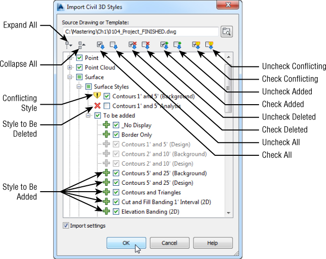
Figure 1.27 Import Civil 3D Styles dialog
The Import Civil 3D Styles dialog has the following options:
- Import SettingsThe Import Settings option is located at the bottom of the dialog. This option is turned on by default. If you want to import the styles with disregard to the drawing settings, then you can uncheck Import Settings. However, if you want to match your drawing in all aspects to the source drawing, you should leave the option checked, which is the default setting. As you look through the list of styles to be imported, you will notice that some items are grayed out and can't be modified.
- The grayed-out styles represent items that are referenced by the command settings to be imported. As mentioned, the only time those styles would not be grayed out and available would be when the Import Settings box is not checked. You will learn about command settings toward the end of this section. Also note that you can either import all the styles from the source drawing or select which styles you want to import.
-
When importing styles, Civil 3D will do the following:
- If the style is not within your drawing, the style will be added.
- If the style already exists in your drawing, presenting the same style name, Civil 3D will recognize it as a conflict of styles and will check its settings against its equivalent in the source file; if the settings are different, they will be overwritten.
- If a style is present in the drawing but not present in the source file, that style will be deleted, as long as it is not used (referenced) by an object in the drawing.
For each of the actions listed here, there is a way to toggle off one or more actions. Following, you can see what happens when you use the toggles:
- Uncheck/Check Conflicting You will also notice items with a warning symbol (see the surface style Contours 1' and 5' (Background) in Figure 1.27). The warning symbol indicates that there is a style in the current drawing with the same name as a style in the batch to be imported. Use the Uncheck Conflicting button if you do not want styles in your drawing to be overwritten by the style from the source file. As mentioned, if you leave these items selected, the incoming styles “win.” If you are not sure whether there is a difference between the styles, pause your cursor over the style name, and a tooltip will tell you what (if any) difference exists.
- Uncheck/Check Added Use the Uncheck Added button if you want only those styles with the same name to come in. Wherever possible, Civil 3D will release items in the To Be Added categories. In cases where a style is used by a setting, you will not be able to uncheck it unless you do not import settings.
- Uncheck/Check Deleted A style in the current drawing will be deleted if the source drawing does not contain a style with the same name and the style is not in use. Use the Uncheck Deleted button to prevent the style from being deleted.
The Import Styles command does not replace the best practice of starting with a proper template. Again, note that some critical items will not get transferred with this tool. As we mentioned, description key sets, unused expressions, point file settings, and predefined point groups will not import. Drawing settings and Label style defaults do not update. In addition, precision and units set in the Feature Settings dialog do not get transferred. The AutoCAD drawing units will remain unchanged, also.
To bring the items that cannot be imported, such as description keys, unused expressions, point file settings, and predefined point groups into your drawing, use the following steps:
- Open the drawing containing the settings or styles you want to import.
- In the same session, open the drawing needing these settings.
- Switch your Toolspace tab to Settings. Make sure your view is set to Master View so that you can see both drawings at the same time.
- Verify that the drawing needing the settings is active.
- On the Settings tab, browse the source drawing for the style or setting you want to import, select the style or setting, and then drag and release it over the drawing area.
Command Settings
We have mentioned command settings many times in this chapter; now you'll learn what they are and their intended purpose. When you create a Civil 3D object, you define its properties, set design parameters, set default styles for objects, and so on. A Civil 3D object is defined through a command. To speed up the standardization of the creation process, the command settings take care of the default values used when a Civil 3D object is created. So, for example, in Figure 1.28 you can see that most of the default settings that the CreateAlignmentLayout tool uses are defined within the command settings. The fact that most of the settings are defined at the drawing level can be seen by the small number of check marks in the Override column.
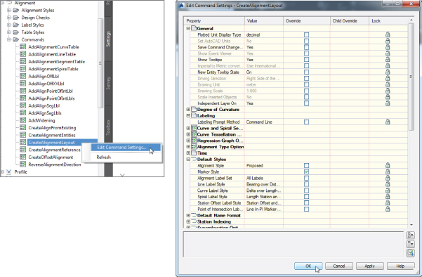
Figure 1.28 Command settings for Create Alignment Layout define the defaults when this tool is used.
You have the option to customize the defaults for the tool so that every time the tool is launched you don't have to type in the same values. Even though the values will be prepopulated in the specific fields, the user still has the option to overwrite those choices within the creation dialog box. Note, however, that only part of the predefined defaults are available to the user within the dialog box. For most of the defaults, the specific command setting dialog is the only place where those values can be defined.
Most of the settings within the command settings are defined on a global level for the drawing within the Ambient Settings tab. Going from a global level to the object level, the same settings can be found and overridden at the object level through the Edit Feature Settings for that type of object. From the object level, you can move to the tool level, where within the command settings for the tool they can again be overridden to achieve the desired settings when using that tool.
Creating Lines
If you have used AutoCAD for a while, you will be familiar with the way you draw lines. Whether you use the command line or the ribbon, the same tools will be available in both Civil 3D and AutoCAD. However, Civil 3D takes it up a notch by providing multiple methods of defining these entities, though the end result will be the same—a line. The tools to draw lines are found in the Draw panel within the Home tab of the ribbon. Figure 1.29 displays the available line commands.
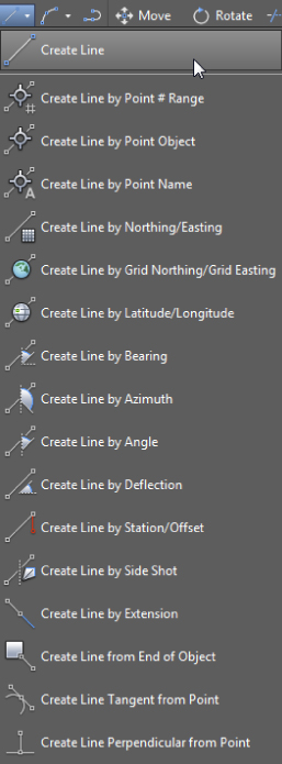
Figure 1.29 Line-creation tools
Later in this chapter you will take a look at transparent commands. Transparent commands provide extra help in the definition of the elements by expanding a user's options of data input within a command.
COGO Line Commands
The next few commands help you create a line using Civil 3D points and/or coordinate inputs. Each command requires you to specify a Civil 3D point, a location in space, or a typed coordinate input. These line tools are useful when your drawing includes Civil 3D points that will serve as a foundation for linework, such as the edge of pavement shots, wetlands lines, or any other points you'd like to connect with a line.
Create Line Command

The Create Line command on the Draw panel of the Home tab of the ribbon issues the standard AutoCAD Line command. It's equivalent to typing line on the command line or clicking the Line tool on the Draw toolbar.
Create Line By Point # Range Command

The Create Line By Point # Range command prompts you for a point number. You can type in an individual point number, press ↲, and then type in another point number. A line is drawn connecting those two points. You can also type in a range of points, such as 601-607. Civil 3D draws a line that connects those points in numerical order from 601 to 607 and so on (see Figure 1.30). The line that is created by this method connects point to point regardless of the description or type of point. Since a line is an element that allows each of its end vertices to hold different elevations, in this case each endpoint will inherit the elevation of the COGO point used for its definition unless the AutoCAD OSNAPZ variable is set to 1.
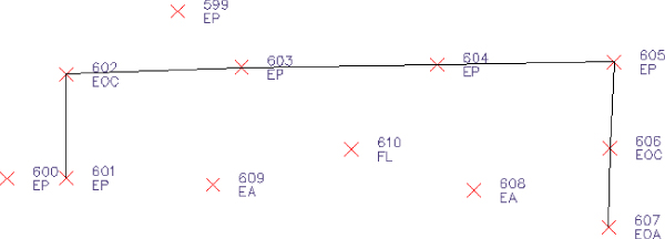
Figure 1.30 Lines created using 601-607 as input
Alternatively, you can enter a list of points such as 600, 603, 610, 605 (Figure 1.31). Civil 3D draws a line that connects the point numbers in the order of input. This approach is useful when your points were taken in a zigzag pattern (as is commonly the case when cross-sectioning pavement) or when your points appear so far apart in the AutoCAD display that they can't be readily identified.
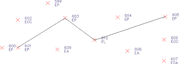
Figure 1.31 Lines created using 600, 603, 610, 605 as input
Create Line By Point Object Command

The Create Line By Point Object command prompts you to select a point object. To select a point object, locate the desired start point and click any part of the point. This tool is similar to using the regular Line command and a Node object snap (also known as an Osnap); however, it will work on only Civil 3D points. Each endpoint will inherit the elevation of the point to which it is created unless the AutoCAD OSNAPZ variable is set to 1.
Create Line By Point Name Command

The Create Line By Point Name command prompts you for a point name. A point name is a field in point properties, not unlike the point number or description. The difference between a point name and a point description is that a point name must be unique, just as point numbers are. It is important to note that some survey instruments name points rather than number points as is the norm.
To use this command, enter the names of the points you want to connect with linework. Each endpoint will inherit the elevation of the point used for its definition unless the AutoCAD OSNAPZ variable is set to 1.
Create Line By Northing/Easting and Create Line By Grid Northing/Grid Easting Commands

The Create Line By Northing/Easting command lets you input northing (y) and easting (x) coordinates as endpoints for your linework.

The Create Line By Grid Northing/Grid Easting command also lets you input grid northing (y) and grid easting (x) coordinates as endpoints for your linework but requires that the drawing have an assigned coordinate system; otherwise, the command resumes to be used as a simple line command.
Create Line By Latitude/Longitude Command

The Create Line By Latitude/Longitude command prompts you for geographic coordinates to use as endpoints for your linework. This command also requires that the drawing have an assigned coordinate system. Enter the latitude and longitude as separate entries at the command line using degrees, minutes, and seconds.
Direction-Based Line Commands
The next few commands help you define a line and its direction. Each of these commands requires you to choose a start point for your line before you can specify the line direction. You can specify your start point by physically choosing a location, using an Osnap, or using one of the point-related line commands discussed earlier.
Many of these line commands require a line or arc and will not work with a polyline. Those commands include Create Line By Sideshot, Create Line By Extension, Create Line From End Of Object, Create Line Tangent From Point, and Create Line Perpendicular From Point.
Create Line By Bearing Command

The Create Line By Bearing command is one of the most commonly used line-creation commands.
This command prompts you for a start point, followed by prompts to input the Quadrant, Bearing, and Distance values. You can enter values on the command line for each input, or you can graphically choose inputs by picking them onscreen. The glyphs at each stage of input guide you in any graphical selections. After creating one line, you can continue drawing lines by bearing, or you can switch to any other method by clicking one of the other Line By commands on the Draw panel (see Figure 1.32).
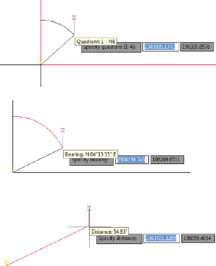
Figure 1.32 The tooltips for a quadrant (top), a bearing (middle), and a distance (bottom)
Create Line By Azimuth Command

The Create Line By Azimuth command prompts you for a start point, followed by a north azimuth and then a distance (Figure 1.33).
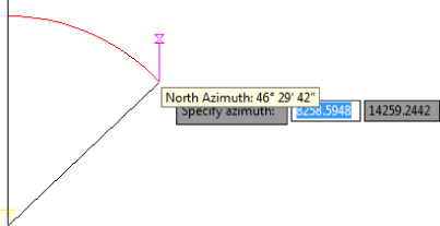
Figure 1.33 The tooltip for the Create Line By Azimuth command
Create Line By Angle Command

The Create Line By Angle command prompts you for a start point, an ending point to establish a backsight direction, a turned angle, and then a distance (Figure 1.34). By default, this command assumes the angle-right surveying convention (clockwise from starting direction). However, an option to turn counterclockwise is offered at the command line if needed.
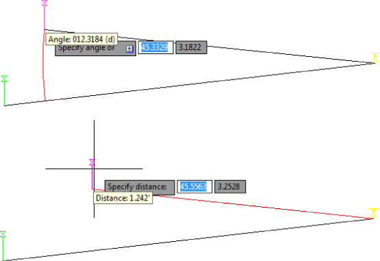
Figure 1.34 The tooltips for a turned angle (top) and a distance (bottom) for the Create Line By Angle command
Create Line By Deflection Command

By definition, a deflection angle is the amount of angular deviation (usually measured clockwise) from a backsight direction. In other words, 180 added to a given deflection angle would be an equivalent angle-right. When you use the Create Line By Deflection command, the command line and tooltips prompt you to define a direction to deflect the angle off of by selecting or clicking two points; then you're prompted for a deflection angle followed by a distance (Figure 1.35).

Figure 1.35 The tooltip for the Create Line By Deflection command
Create Line By Station/Offset Command

To use the Create Line By Station/Offset command, you must have a Civil 3D Alignment object in your drawing. The line created from this command allows you to start and end a line on the basis of a station and offset from an alignment.
You're prompted to choose the alignment and then input a station and offset value. The line begins at the station and offset value. You will not see a line form until at least two points are specified.
When prompted for the station, you're given a tooltip that tracks your position along the alignment, as shown in Figure 1.36. You can graphically choose a station location by clicking it in the drawing. Alternatively, you can enter a station value on the command line.
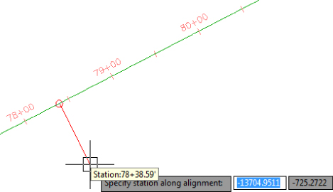
Figure 1.36 The Create Line By Station/Offset command provides a tooltip for you to track stationing along the alignment.
Once you've selected the station, you're given a tooltip that is locked on that particular station and tracks your offset from the alignment (see Figure 1.37). You can graphically choose an offset by clicking the station in the drawing, or you can type an offset value on the command line. A negative value for offset indicates an offset on the left side of the alignment.
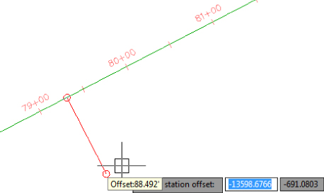
Figure 1.37 The Create Line By Station/Offset command provides a tooltip that helps you track the offset from the alignment.
Create Line By Side Shot Command

The Create Line By Side Shot command starts by asking you to select a line (or two points) that will be the backsight for creating a new line and subsequent lines while in the command. After you select the first line, you will see a yellow glyph indicating your occupied point (see Figure 1.38). By default, Civil 3D is looking for an angle-right and distance to establish the first point of the new line. However, you can follow the command prompts to change the angle entry to bearing, deflection, or azimuth, if needed. You can also use the command-line options to change to counterclockwise.

Figure 1.38 The tooltip for the Create Line By Side Shot command tracks the angle, bearing, deflection, or azimuth of the side shot.
Once you have entered data for the first point, you will be asked a second time for an angle and a distance to place the second point of the new line.
Create Line By Extension Command

The Create Line By Extension command is similar to the AutoCAD Lengthen command. This command allows you to add length to a line or specify a desired total length of the line. Figure 1.39 shows the summary report that will pop up indicating the changes made to the line.
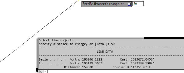
Figure 1.39 The Create Line By Extension command provides a summary of the changes to the line.
The advantage of the Create Line By Extension command over simply using the Lengthen command is the summary report that appears at the command line. The summary report shown in Figure 1.40 shows the same beginning coordinate as in Figure 1.39 but a different end coordinate, resulting in a total length of 100' (30.5 m).

Figure 1.40 The summary report on a line where the command specified a total distance
Create Line From End Of Object Command

The Create Line From End Of Object command lets you draw a line tangent to the end of a line or arc (but not polyline) of your choosing, as shown in Figure 1.41.

Figure 1.41 The Create Line From End Of Object command lets you add a tangent line to the end of an arc.
Create Line Tangent From Point Command

The Create Line Tangent From Point command is similar to the Create Line From End Of Object command, but Create Line Tangent From Point allows you to choose a point of tangency that isn't the endpoint of the line or arc. Use the Nearest or Midpoint Osnap to pick a point on the line. If you pick an endpoint, the command behaves the same as Create Line From End Of Object.
Create Line Perpendicular From Point Command

Using the Create Line Perpendicular From Point command, you can specify that you'd like a line drawn perpendicular to any point of your choosing along a line or arc. In the example shown in Figure 1.42, a line is drawn perpendicular to the endpoint of the arc.

Figure 1.42 A perpendicular line is drawn from the endpoint of an arc using the Create Line Perpendicular From Point command.
Re-Creating a Deed Using Line Tools
The upcoming exercise will help you apply some of the tools you've learned so far to reconstruct the overall parcel.
When you open the file for the exercise, you will see a legal description with the following information (the metric file will have different lengths, of course):
From the POINT OF BEGINNING at a location of N 186156.65', E 2305474.07'
Thence, S 11° 45' 41.4" E for a distance of 693.77 feet to a point on a line.
Thence, S 73° 10' 54.4" W for a distance of 265.45 feet to a point on a line.
Thence, S 05° 59' 04.4" E for a distance of 185.89 feet to a point on a line.
Thence, S 45° 55' 02.4" W for a distance of 68.73 feet to a point on a line.
Thence, N 06° 04' 37.0" W for a distance of 217.80 feet to a point on a line.
Thence, N 73° 21' 22.5" E for a distance of 4.22 feet to a point on a line.
Thence, N 06° 04' 51.6" W for a distance of 200.14 feet to a point on a line.
Thence, S 87° 32' 10.4" W for a distance of 121.22 feet to a point on a line.
Thence, N 02° 25' 32.2" W for a distance of 168.91 feet to a point on a line.
Thence, N 15° 38' 57.5" E for a distance of 283.16 feet to a point on a line.
Thence, N 06° 19' 22.4" W for a distance of 79.64 feet to a point on a line.
N 76° 55' 49.8" E a distance of 250.00 feet Returning to the POINT OF BEGINNING;
Containing 5.58 acres (more or less)
Follow these steps (note that the legal description for metric users is located in the DWG file as text):
- Open the
0106_Legal.dwg(0106_Legal_METRIC.dwg) file, which you can download from this book's web page atwww.sybex.com/go/masteringcivil3d2016. - Turn off dynamic input by pressing F12 if it is enabled.
- From the Draw panel on the Home tab of the ribbon, select the Line drop-down and choose the Create Line By Bearing command.
- At the
Select first point: prompt, use endpoint object snap to snap to the arrow head of the note indicating POB. - At the
≫Specify quadrant (1-4): prompt, enter 2 to specify the SE quadrant and then press ↲ - At the
≫Specify bearing: prompt, enter 11.45414 and press ↲. - At the
≫Specify distance: prompt, enter 693.77' (211.4615 m) and press ↲. - Repeat steps 5 through 7 for the rest of the courses and distances.
- Press Esc twice to exit the creation workflow and exit the Create Line By Bearing command.
The finished linework should look like Figure 1.43.
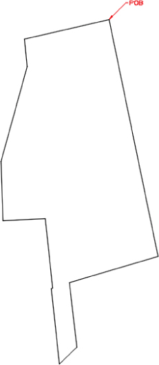
Figure 1.43 The finished linework
- Save your drawing. You'll need it for the next exercise.
Creating Curves
Curves are an important part of surveying and engineering geometry. The curves you create in this chapter are no different from AutoCAD arcs. What makes the curve commands unique from the basic AutoCAD commands isn't the resulting arc entity but the inputs used to draw the arc. Civil 3D wants you to provide directions to the arc commands using land surveying terminology rather than with generic Cartesian parameters. Figure 1.44 shows the Create Curves menu options.

Figure 1.44 Create Curves commands
Standard Curves
When re-creating legal descriptions for roads, easements, and properties, users such as engineers, surveyors, and mappers often encounter a variety of curves. Although standard AutoCAD arc commands could draw these arcs, the AutoCAD arc inputs are designed to be generic to all industries. The following curve commands have been designed to provide an interface that more closely matches land surveying, mapping, and engineering language.
Creating a Curve Between Two Lines

The Create Curve Between Two Lines command is similar to the AutoCAD Fillet command, except that by using this tool you also have other options to define a curve besides using the radius. The command draws a curve that is tangent to two lines of your choosing. This command also trims or extends the original tangents so their endpoints coincide with the curve endpoints. The lines are trimmed or extended to the resulting PC (point of curve, which is the beginning of a curve) and PT (point of tangency, which is the end of a curve). You may find this command most useful when you're creating foundation geometry for road alignments, parcel boundary curves, and similar situations.
The command prompts you to choose the first tangent and then the second tangent. The command line gives the following prompt:
Select entry [Tangent External Degree Chord Length Mid-ordinate
miN-dist Radius]<Radius>:
Pressing ↲ at this prompt lets you input your desired radius. As with standard AutoCAD commands, pressing T changes the input parameter to Tangent, pressing C changes the input parameter to Chord, and so on.
As with the Fillet command, your inputs must be geometrically possible. For example, your two lines must allow for a curve of your specifications to be drawn while remaining tangent to both. Figure 1.45 shows two lines with a 25' (7.6 m) radius curve drawn between them. Note that the tangents have been trimmed so their endpoints coincide with the endpoints of the curve. If either line is too short to meet the endpoint of the curve, then the software returns a no solution result, and you will need to adjust the length of the line.
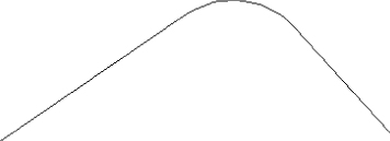
Figure 1.45 Two lines using the Create Curve Between Two Lines command
Creating a Curve on Two Lines
The Create Curve On Two Lines command is identical to the Create Curve Between Two Lines command, except that in this case the tangents are not trimmed on curve creation.

Figure 1.46, for example, shows two lines with a 25' (7.6 m) radius curve drawn on them. The tangents haven't been trimmed and instead remain exactly as they were drawn before the Create Curve On Two Lines command was executed.
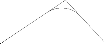
Figure 1.46 The original lines stay the same after you execute the Create Curve On Two Lines command.
Creating a Curve-Through Point

The Create Curve Through Point command lets you choose two tangents for your curve followed by a pass-through point. This tool is most useful when you don't know the radius, length, or other curve parameters but you have two tangents and a target location. It isn't necessary that the pass-through location be a true point object; it can be any location of your choosing.
This command also trims or extends the original tangents so their endpoints coincide with the curve endpoints. The lines are trimmed or extended to the resulting PC and PT of the curve.
Figure 1.47, for example, shows two lines and a desired pass-through point. Using the Create Curve Through Point command allows you to draw a curve that is tangent to both lines and that passes through the desired point. In this case, the tangents have been trimmed to the PC and PT of the curve.
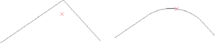
Figure 1.47 The first image shows two lines with a desired pass-through point. In the second image, the Create Curve Through Point command draws a curve that is tangent to both lines and passes through the chosen point.
Creating Multiple Curves

The Create Multiple Curves command lets you create several curves that are tangentially connected. The resulting curves have an effect similar to an alignment spiral section. This command can be useful when you are re-creating railway track geometry based on field-survey data.
The command prompts you for the two tangents. Then, the command line prompts you as follows:
Enter Number of Curves:The command allows for up to 10 curves between tangents.
One of your curves must have a flexible length that's determined on the basis of the lengths, radii, and geometric constraints of the other curves. Curves are counted clockwise, so enter the number of your flexible curve, as shown here:
Enter Floating Curve #:
Enter curve 1 Radius:
Enter curve 2 Radius:
Enter curve 2 Length:
The floating curve number will prompt you for a radius but not a length.
As with all other curve commands, the specified geometry must be possible. If the command can't find a solution on the basis of your length and radius inputs, it returns no solution (see Figure 1.48).
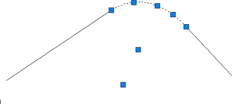
Figure 1.48 Two curves were specified with the #2 curve designated as the floating curve.
Creating a Curve from the End of an Object

The Create Curve From End Of Object command enables you to draw a curve tangent to the end of your chosen line or arc.
The command prompts you to choose an object to serve as the beginning of your curve. You can then specify a radius or a point for the way the curve will be defined. If a point is selected, then the curve will automatically be drawn ending at the selected point in the drawing. If a radius is selected, then you have the option to specify the radius or let the software determine the radius based on the arc's degree or the chord's degree. Finally, you can define its length by using an additional parameter (such as Delta or Length) (see Figure 1.49).
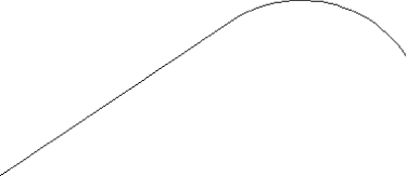
Figure 1.49 A curve, with a 25′ (7.6 m) radius and a 30′ (9.1 m) length, drawn from the end of a line
Creating a Reverse or Compound Curve

The Create Reverse Or Compound Curve command allows you to add curves to the end of an existing curve. Reverse curves are drawn in the opposite direction (that is, a curve to the right tangent to a curve to the left) from the original curve to form an S shape. In contrast, compound curves are drawn in the same direction as the original curve (see Figure 1.50). This tool can be useful when you are re-creating a legal description of a road alignment that contains reverse and/or compound curves.
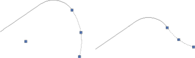
Figure 1.50 A tangent and curve before adding a compound curve (left); a reverse curve drawn from the end of the original curve (right)
Using the Curve Calculator

Sometimes you may not have enough information to draw a curve properly. Although many of the curve-creation tools assist you in calculating the curve parameters, you may find an occasion where the deed you're working with is incomplete.
The Curve Calculator found in the Curves drop-down on the Draw panel helps you calculate a full collection of curve parameters on the basis of your known values and constraints. It can also be found as part of the Transparent Commands toolbar that is discussed later in this chapter.
The Curve Calculator can remain open on your screen while you're working through commands. You can send any value in the Calculator to the command line by clicking the button next to that value (see Figure 1.51).
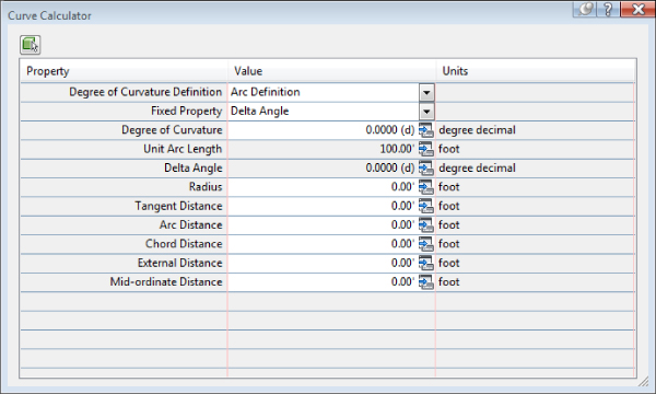
Figure 1.51 The Curve Calculator
The button at the upper left of the Curve Calculator allows you to pick an existing arc in the drawing, and the drop-down menu in the Degree Of Curvature Definition selection field allows you to choose whether to calculate parameters for an arc or a chord definition.
The drop-down menu in the Fixed Property selection field also gives you the choice of fixing your radius or delta angle when calculating the values for an arc or a chord, respectively. The parameter chosen as the fixed value is held constant as additional parameters are calculated.

To send any value in the Curve Calculator to the command line, use the button next to that value. This ability is most useful while you're active in a curve command and would like to use a certain parameter value to complete the command.
To test your new line and curve knowledge, follow these steps (you do not need to have completed the previous exercises to complete this one):
- Continue working in the file
0106_Legal.dwg(0106_Legal_METRIC.dwg). - Start the Line By Northing/Easting command.
- For Northing, enter 184898.42 (56357.038 for metric users) and press ↲.

- For Easting, enter 2305136.46 (702605.593 for metric users) and press ↲.
You will not see any graphic indication that the line has been started. You will not see the segment until after you complete step 5.
You will again be prompted for Northing and Easting.
- Using the same procedure you used in step 2, type in the endpoint of the line at Northing = 185059.94 (56406.270 for metric users), Easting = 2305413.52 (702690.041 for metric users).
- Press Esc once to end the Northing and Easting entries.
- Press Esc again to exit the line command.
To look at everything you have drawn until now, you can zoom to extents.
- Start the Create Curve From End Of Object command.

You are then prompted to select the Line or Arc object.
- Pan to the left and click the east end of the line you created in steps 2–5.
You will then be prompted to select the entry.
- Press ↲ to select the default Radius option.
- Enter a Radius value of 550' (167.6 m) and press ↲.
Next you will see the
Select entry [Tangent/Chord/Delta/Length/External/Mid-ordinate] <Length>: prompt. - Enter D (for Delta) and press ↲.
- Enter a delta angle of 40 and press ↲. (Note: The degree symbol is not needed in angular entry.)
You should now have an arc tangent to the first segment.
- Return to the Curves menu and select Create Reverse Or Compound Curve.

- Select the east end of the arc you created in the previous steps.
- When prompted with
Select [Compound/Reverse] <Compound>:, press R and then ↲ to specify a reverse curve. - Enter a radius of 630' (192.0 m) and press ↲.
- When you see the prompt
Select entry [Tangent/Chord/Delta/Length/External/Mid-ordinate] <Length>:, press ↲ to accept the default. - Enter a length of curve value of 400' (121.9 m) and press ↲.
- For the last tangent segment, return to the Lines menu and select Create Line From End Of Object.

- Select the east end of the second arc you created in this exercise.
- At the
Specify Distance: prompt, enter 150' (45.7 m) and press ↲.
Your completed lines and arcs will look like Figure 1.52, and they will be located just south of the property you entered in the previous exercise. You can check the result against the completed exercise as found on the book's web page; it's named 0106_Legal_FINISHED.dwg (0106_Legal_METRIC_FINISHED.dwg).
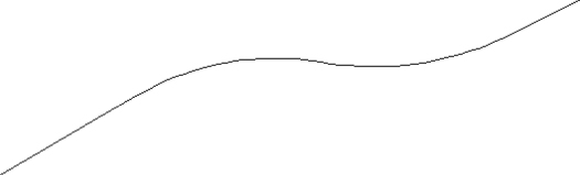
Figure 1.52 Lines and arcs of the completed exercise
Best-Fit Entities
AutoCAD Civil 3D provides many tools for relating surveyed information to a graphic. Best-fit tools like the ones in the following sections perform analysis on different types of irregular geometry to create uniform shapes (see Figure 1.53). Similar tools are available for alignment creation, as discussed in Chapter 6.
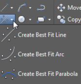
Figure 1.53 The Create Best Fit menu options
Creating a Best-Fit Line

The Create Best Fit Line command under the Best Fit drop-down on the Draw panel takes a series of Civil 3D points, AutoCAD points, entities, or drawing locations and draws a single best-fit line segment on the selected input. In Figure 1.54, the Create Best Fit Line command draws a best-fit line through a series of points that aren't quite collinear. The best-fit line will adjust as more points are selected.
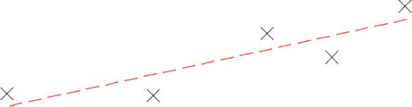
Figure 1.54 A preview line drawn through points that are not collinear
After you press Enter to complete the selection, a Panorama window appears with a regression data chart showing information about each point in the selection, as shown in Figure 1.55.
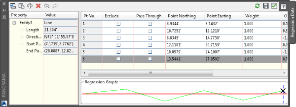
Figure 1.55 The Panorama window lets you optimize your best fit.
This interface allows you to optimize your best-fit element by adding more points, excluding points, selecting the check box in the Pass Through column to force one of your points on the line, or adjusting the value under the Weight column based on how important each point position should be in the definition of the element relative to the other points.
Creating a Best-Fit Arc

The Create Best Fit Arc command on the Best Fit drop-down works the same as the Create Best Fit Line command, including the Panorama adjustment window, except that the resulting entity is a single arc segment as opposed to a single line segment (see Figure 1.56).

Figure 1.56 Preview of the curve created by best fit
Creating a Best-Fit Parabola

The Create Best Fit Parabola command on the Best Fit drop-down is similar to the line and arc commands in how it works. After you select this command, the Parabola By Best Fit dialog appears (see Figure 1.57).

Figure 1.57 The Parabola By Best Fit dialog
You can select inputs from entities (such as lines, arcs, polylines, or profile objects) or by clicking onscreen. The command then draws a best-fit parabola on the basis of this information. In Figure 1.58, the shots were represented by AutoCAD points; more points were added by selecting the By Clicking On The Screen option and using the Node Osnap to pick each point.
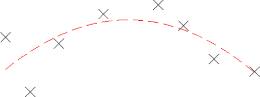
Figure 1.58 The best-fit preview line updates as more points are picked.
Once you've selected your points, a Panorama window (shown in Figure 1.59) appears, showing information about each point you chose. Also note the information in the left pane regarding the K value, curve length, grades, and so forth. You can optimize your K value, length, and other values by adding more points, selecting one or more check boxes in the Pass Through column to force one of your points on the line, or adjusting the values in the Weight column.
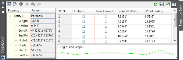
Figure 1.59 The Panorama window lets you make adjustments to your best-fit parabola.
Attaching Multiple Entities

The Attach Multiple Entities command that can be called out in the command line as attachmultiple is a combination of the Line From End Of Object command and the Curve From End Of Object command. Using CUI, you can bring this command into the ribbon if desired. Each entity created with this tool is tangent to the previous segment. Using this command saves you time because you don't have to switch between the Line From End Of Object command and the Curve From End Of Object command (see Figure 1.60).
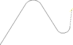
Figure 1.60 The Attach Multiple Entities command draws a series of lines and arcs so that each segment is tangent to the previous one.
Adding Line and Curve Labels
In Civil 3D the dynamic and intelligent labeling is not limited to Civil 3D objects alone. You can add dynamic linked labels to basic AutoCAD elements like lines and curves. These labels share the most common properties of the labels used for other Civil 3D objects such as parcels and alignments.
This exercise leads you through labeling the deed you entered earlier in this chapter:
- Open the file
0107_Legal_Labels.dwg(0107_Legal_Labels_METRIC.dwg), which can be downloaded from the book's web page. - On the Annotate tab of the ribbon, choose Labels And Tables Panel Add Labels.
The Add Labels dialog appears.

- Choose Line And Curve from the Feature drop-down menu.
Your Add Labels dialog will look similar to Figure 1.61.
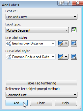
Figure 1.61 The Add Labels dialog, with Label Type set to Multiple Segment
- Choose Multiple Segment from the Label Type drop-down menu.
The Multiple Segment option places the label at the midpoint of each selected line or arc.
- Confirm that Line Label Style is set to Bearing Over Distance and that Curve Label Style is set to Distance-Radius And Delta (as shown in Figure 1.61).
- Click the Add button.
- At the
Select Entity: prompt, select each line from the deed and the lines and arcs that you drew in the previous exercises.A label appears on each entity at its midpoint, as shown in Figure 1.62.
- Save the drawing and close it.
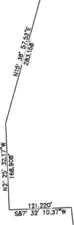
Figure 1.62 The labeled linework
You can check the result of your drawing against the completed file found on the web page for the book; it's named 0107_Legal_Labels_FINISHED.dwg (0107_Legal_Labels_METRIC_FINISHED.dwg).
The use of these labels does not stop at lines and curves; they can be used on polylines as well. Based on the selection of a single segment or multiple segments, Civil 3D can apply the labels to a single segment on the polyline or all segments of the polyline, assigning the specific label to lines and curves that define the polyline.
Using Transparent Commands
You might be surprised to know that you have already been using a form of the transparent commands if you tried to use, for example, the Line By Point # Range command or the Line By Bearing command. That's because each of those commands is a variation of the line command with a transparent command already built in.
Transparent commands are “helper” commands that make base AutoCAD input more surveyor- and civil designer–friendly. Transparent commands can be used only when another command is in progress. They are “commands within commands” that allow you to choose your input based on the available data you have to provide.
For example, you may have a plat whose information you are trying to input into AutoCAD. You may need to insert a block at a specific northing and easting. While the Line command has a built-in option for Northing Easting, the Insert command does not, and a transparent command will help you. In this case, you would start the Insert command with the Specify On Screen option checked. Before you click to place the block in the graphic, click the Northing Easting transparent command. The command line will then walk you through placing the block at your desired location.
While a transparent command is active, you can press Esc once to leave transparent mode but stay active in your current command. You can then choose another transparent command if you'd like. For example, you can start a line using the Endpoint Osnap, activate the Angle Distance transparent command, draw a line-by-angle distance, and then press Esc, which takes you out of angle-distance mode but keeps you in the line command. You can then draw a few more segments using the Point Object transparent command, press Esc, and finish your line with a Perpendicular Osnap.
You can activate the transparent commands using keyboard shortcuts or the Transparent Commands toolbar. Be sure you include the Transparent Commands toolbar (shown in Figure 1.63) in all your Civil 3D and survey-oriented workspaces.
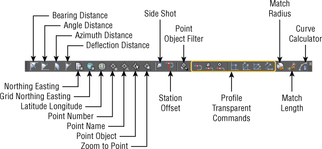
Figure 1.63 The Transparent Commands toolbar
The seven profile-related transparent commands will be covered in Chapter 7.
Standard Transparent Commands
The transparent commands shown in Table 1.2 can be called out within any AutoCAD or Civil 3D draw command, such as a line, polyline, alignment, parcel segment, feature line, or pipe-creation command.
Table 1.2 The transparent commands used in plan view
| Tool Icon | Menu Command | Key-In | Tool Icon | Menu Command | Key-In |
 |
Angle Distance | ‘AD |  |
Latitude Longitude | ‘LL |
 |
Bearing Distance | ‘BD |  |
Point Number | ‘PN |
 |
Azimuth Distance | ‘ZD |  |
Point Name | ‘PA |
 |
Deflection Distance | ‘DD |  |
Point Object | ‘PO |
 |
Northing Easting | ‘NE |  |
Zoom To Point | ‘ZTP |
 |
Grid Northing Grid Easting | ‘GN |  |
Side Shot | ‘SS |
 |
Station Offset | ‘SO |
Matching Transparent Commands
You may have construction or other geometry in your drawing that you'd like to match with new lines, arcs, circles, alignments, parcel segments, or other entities.

While actively drawing an object that has a radius parameter, such as a circle, an arc, an alignment curve, or a similar object, you can choose the Match Radius transparent command and then select an object in your drawing that has your desired radius. Civil 3D draws the resulting entity with a radius identical to that of the object you chose during the command.

The Match Length transparent command works the same as the Match Radius transparent command except that it matches the length parameter of your chosen object.
Some people find working with transparent commands awkward at first. It feels strange to move your mouse away from the drawing area and click an icon while another command is in progress. If you prefer, each transparent command has a corresponding command-line entry.
Try a few transparent commands to get the feel for how they operate.
- Open the drawing
0108_Transparent_Commands.dwg(0108_Transparent_Commands_METRIC.dwg). - On the Home tab of the ribbon, click the Draw flyout 3D Polyline.

- From the Transparent Commands toolbar, click the Point Number Transparent command.

- At the Enter Point Number prompt, type 100-112 and press ↲.
The 3D polyline will connect the points in the drawing.
- Press Esc once.
Notice that you are now back in the 3D polyline command with no transparent commands active.
- Press Esc a second time.
This will exit the 3D polyline command.
- On the Insert tab Block panel Insert flyout More Options.

- From the Name pull-down, select the block Fire Hydrant 01.
You do not need to browse because this block is already defined in this example drawing.
- Check the Specify On-Screen option for Insertion Point.
- Uncheck the Explode option.
- Verify that your settings match what is shown in Figure 1.64 and click OK.
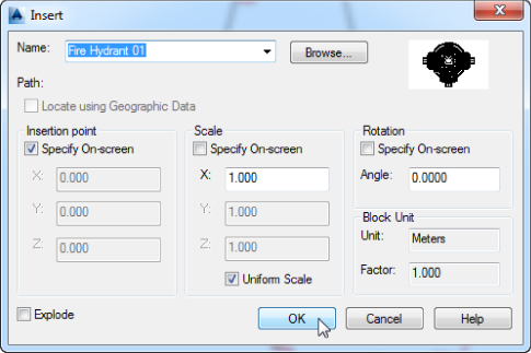
Figure 1.64 Using the Insert command to place a block
- At the
Specify insertion point: prompt, select the Station Offset transparent command.You are then prompted to select an alignment.

- Click the alignment to the south of the site. (Hint: Be sure to click the green line rather than the labels.)
- At the
Specify station along alignment: prompt, enter 450’ (175 m) and press ↲. - At the
Specify station offset: prompt, enter −30’ (−10 m) and press ↲.
You should now see the fire hydrant symbol at the specified station, on the left of the alignment. You can go ahead and save the drawing, and you can compare the final result against the completed file as found on the web page for the book under the name 0108_Transparent_Commands_FINISHED.dwg (0108_Transparent_Commands_METRIC_FINISHED.dwg).
The Bottom Line
- Find any Civil 3D object with just a few clicks. By using Prospector to view object data collections, you can minimize the panning and zooming that are part of working in a CAD program. When common subdivisions can have hundreds of parcels or a complex corridor can have dozens of alignments, jumping to the desired one nearly instantly shaves time off everyday tasks.
- Master It Open
0103_Example.dwg(0103_Example_METRIC.dwg) fromwww.sybex.com/go/masteringcivil3d2016and find parcel number 6 without using any AutoCAD commands or scrolling around on the drawing screen.
- Master It Open
- Modify the drawing scale and default object layers. Civil 3D understands that the end goal of most drawings is to create hard-copy construction documents. When you set a drawing scale, Civil 3D removes a lot of the mental gymnastics that other programs require when you're sizing text and symbols. When you set object layers for the entire drawing, Civil 3D makes uniformity of drawing files easier than ever to accomplish.
- Master It Continue working in the file
0103_Example.dwg(0103_Example_METRIC.dwg). It is not necessary to have completed the previous exercise to continue. Zoom to extents and change the Annotation scale in the Model tab from the 50-scale drawing to a 100-scale drawing. (For metric users, change the scale from 1:250 to 1:1000.)
- Master It Continue working in the file
- Navigate the ribbon's contextual tabs. As with AutoCAD, the ribbon is the primary interface for accessing Civil 3D commands and features. When you select an AutoCAD Civil 3D object, the ribbon displays commands and features related to that object. If several object types are selected, the Multiple contextual tab is displayed.
- Master It Continue working in the file
0103_Example.dwg(0103_Example_METRIC.dwg). It is not necessary to have completed the previous exercise to continue. Using the ribbon interface, access the Alignment properties for QuickStart Alignment and rename it Existing CL.
- Master It Continue working in the file
- Create a curve tangent to the end of a line. It's rare that a property stands alone. Often, you must create adjacent properties, easements, or alignments from their legal descriptions.
- Master It Open the drawing
MasterIt_0101.dwg(MasterIt_0101_METRIC.dwg). Create a curve tangent to the east end of the line labeled in the drawing. The curve should meet the following specifications:- Radius: 200.00’ (60 m)
- Arc Length: 66.58’ (20 m)
- Master It Open the drawing
- Label lines and curves. Although converting linework to parcels or alignments offers you the most robust labeling and analysis options, basic line- and curve-labeling tools are available when conversion isn't appropriate.
- Master It Add line and curve labels to each entity created in
MasterIt_0101.dwgorMasterIt_0101_METRIC.dwg. It is recommended that you complete the previous exercise so you will have a curve to work with. Choose a label that specifies the bearing and distance for your lines and length, radius, and delta of your curve. Check your final result against the completed file found on the book's web page namedMasterIt_0101_FINISHED.dwg(MasterIt_0101_METRIC_FINISHED.dwg).
- Master It Add line and curve labels to each entity created in