Chapter 4

Big data analytics

Having discussed how big data is collected and stored, we can now look at some of the techniques used to discover useful information from that data such as customer preferences or how fast an epidemic is spreading. Big data analytics, the catch-all term for these techniques, is changing rapidly as the size of the datasets increases and classical statistics makes room for this new paradigm.

Hadoop, introduced in Chapter 3, provides a means for storing big data through its distributed file system. As an example of big data analytics we’ll look at MapReduce, which is a distributed data processing system and forms part of the core functionality of the Hadoop Ecosystem. Amazon, Google, Facebook, and many other organizations use Hadoop to store and process their data.

MapReduce

A popular way of dealing with big data is to divide it up into small chunks and then process each of these individually, which is basically what MapReduce does by spreading the required calculations or queries over many, many computers. It’s well worth working through a much simplified and reduced example of how MapReduce works—and as we are doing this by hand it really will need to be a considerably reduced example, but it will still demonstrate the process that would be used for big data. There would be typically many thousands of processors used to process a huge amount of data in parallel, but the process is scalable and it’s actually a very ingenious idea and simple to follow.

There are several parts to this analytics model: the map component; the shuffle step; and the reduce component. The map component is written by the user and sorts the data we are interested in. The shuffle step, which is part of the main Hadoop MapReduce code, then groups the data by key, and finally we have the reduce component, which again is provided by the user, which aggregates these groups and produces the result. The result is then sent to HDFS for storage.

For example, suppose we have the following key−value files stored in the Hadoop distributed file system, with statistics on each of the following: measles, Zika virus, TB, and Ebola. The disease is the key and a value representing the number of cases for each disease is given. We are interested in the total number of cases of each disease.

File 1:

Measles,3

Zika,2 TB,1 Measles,1

Zika,3 Ebola,2

File 2:

Measles,4

Zika,2 TB,1

File 3:

Measles,3 Zika,2

Measles,4 Zika,1 Ebola,3

The mapper enables us to read each of these input files separately, line by line, as shown in Figure 11. The mapper then returns the key−value pairs for each of these distinct lines.

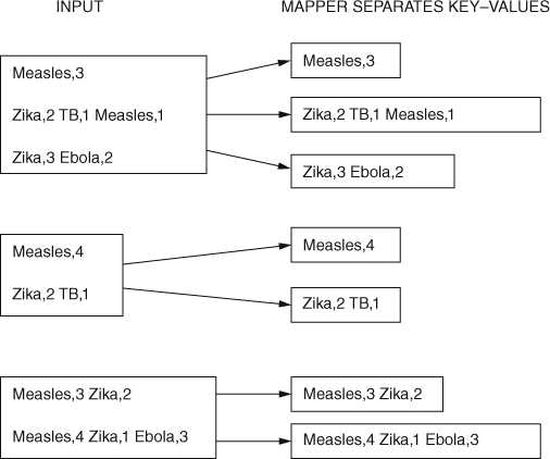
11. Map function.

Having split the files and found key−values for each split, the next step in the algorithm is provided by the master program, which sorts and shuffles the key−values. The diseases are sorted alphabetically and the result is sent to an appropriate file ready for the reducer, as shown in Figure 12.

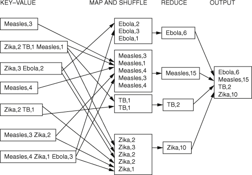
12. Shuffle and reduce functions.

Continuing to follow Figure 12, the reduce component combines the results of the map and shuffle stages, and as a result sends each disease to a separate file. The reduce step in the algorithm then allows the individual totals to be calculated and these results are sent to a final output file, as key−value pairs, which can be saved in the DFS.

This is a very small example, but the MapReduce method enables us to analyse very large amounts of data. For example, using the data supplied by Common Crawl, a non-profit organization that provides a free copy of the Internet, we could count the number of times each word occurs on the Internet by writing a suitable computer program that uses MapReduce.

Bloom filters

A particularly useful method for mining big data is the Bloom filter, a technique based on probability theory which was developed in the 1970s. As we will see, Bloom filters are particularly suited to applications where storage is an issue and where the data can be thought of as a list.

The basic idea behind Bloom filters is that we want to build a system, based on a list of data elements, to answer the question ‘Is X in the list?’ With big datasets, searching through the entire set may be too slow to be useful, so we use a Bloom filter which, being a probabilistic method, is not 100 per cent accurate—the algorithm may decide that an element belongs to the list when actually it does not; but it is a fast, reliable, and storage efficient method of extracting useful knowledge from data.

Bloom filters have many applications. For example, they can be used to check whether a particular Web address leads to a malicious website. In this case, the Bloom filter would act as a blacklist of known malicious URLs against which it is possible to check, quickly and accurately, whether it is likely that the one you have just clicked on is safe or not. Web addresses newly found to be malicious can be added to the blacklist. Since there are now over a billion websites, and more being added daily, keeping track of malicious sites is a big data problem.

A related example is that of malicious email messages, which may be spam or may contain phishing attempts. A Bloom filter provides us with a quick way of checking each email address and hence we would be able to issue a timely warning if appropriate. Each address occupies approximately 20 bytes, so storing and checking each of them becomes prohibitively time-consuming since we need to do this very quickly—by using a Bloom filter we are able to reduce the amount of stored data dramatically. We can see how this works by following the process of building a small Bloom filter and showing how it would function.

Suppose we have the following list of email addresses that we want to flag as malicious: <aaa@aaaa.com>; <bbb@nnnn.com>; <ccc@ff.com>; <dd@ggg.com>. To build our Bloom filter first assume we have 10 bits of memory available on a computer. This is called a bit array and initially it is empty. A bit has just two states, usually denoted by 0 and 1, so we will start by setting all values in the bit array to 0, meaning empty. As we will see shortly, a bit with a value of 1 will mean the associated index has been assigned at least once.

The size of our bit array is fixed and will remain the same regardless of how many cases we add. We index each bit in the array as shown in Figure 13.

13. 10-bit array.

We now need to introduce hash functions, which are algorithms designed to map each element in a given list to one of the positions in the array. By doing this, we now store only the mapped position in the array, rather than the email address itself, so that the amount of storage space required is reduced.

For our demonstration, we show the result of using two hash functions, but typically seventeen or eighteen functions would be used together with a much bigger array. Since these functions are designed to map more or less uniformly, each index has an equal chance of being the result each time the hash algorithm is applied to a different address.

So, first we let the hash algorithms assign each email address to one of the indices of the array.

To add ‘aaa@aaaa.com’ to the array, it is first passed through hash function 1, which returns an array index or position value. For example, let’s say hash function 1 returned index 3. Hash function 2, again applied to ‘aaa@aaaa.com’, returned index 4. These two positions will each have their stored bit value set to 1. If the position was already set to 1 then it would be left alone. Similarly, adding ‘bbb@nnnn.com’ may result in positions 2 and 7 being occupied or set to 1 and ‘ccc@ff.com’ may return positions 4 and 7. Finally, assume the hash functions applied to ‘dd@ggg.com’ return the positions 2 and 6. These results are summarized in Figure 14.

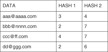
14. Summary of hash function results.

The actual Bloom filter array is shown in Figure 15 with occupied positions having a value set to 1.

15. Bloom filter for malicious email addresses.

So, how do we use this array as a Bloom filter? Suppose, now, that we receive an email and we wish to check whether the address appears on the malicious email address list. Suppose it maps to positions 2 and 7, both of which have value 1. Because all values returned are equal to 1 it probably belongs to the list and so is probably malicious. We cannot say for certain that it belongs to the list because positions 2 and 7 have been the result of mapping other addresses and indexes may be used more than once. So the result of testing an element for list membership also includes the probability of returning a false positive. However, if an array index with value 0 is returned by any hash function (and, remember, there would generally be seventeen or eighteen functions) we would then definitely know that the address was not on the list.

The mathematics involved is complex but we can see that the bigger the array the more unoccupied spaces there will be and the less chance of a false positive result or incorrect matching. Obviously the size of the array will be determined by the number of keys and hash functions used, but it must be big enough to allow a sufficient number of unoccupied spaces for the filter to function effectively and minimize the number of false positives.

Bloom filters are fast and they can provide a very useful way of detecting fraudulent credit card transactions. The filter checks to see whether or not a particular item belongs to a given list or set, so an unusual transaction would be flagged as not belonging to the list of your usual transactions. For example if you have never purchased mountaineering equipment on your credit card, a Bloom filter will flag the purchase of a climbing rope as suspicious. On the other hand, if you do buy mountaineering equipment, the Bloom filter will identify this purchase as probably acceptable but there will be a probability that the result is actually false.

Bloom filters can also be used for filtering email for spam. Spam filters provide a good example since we do not know exactly what we are looking for—often we are looking for patterns, so if we want email messages containing the word ‘mouse’ to be treated as spam we also want variations like ‘m0use’ and ‘mou$e’ to be treated as spam. In fact, we want all possible, identifiable variations of the word to be identified as spam. It is much easier to filter everything that does not match with a given word, so we would only allow ‘mouse’ to pass through the filter.

Bloom filters are also used to speed up the algorithms used for Web query rankings, a topic of considerable interest to those who have websites to promote.

PageRank

When we search on Google, the websites returned are ranked according to their relevance to the search terms. Google achieves this ordering primarily by applying an algorithm called PageRank. The name PageRank is popularly believed to have been chosen after Larry Page, one of the founders of Google, who, working with co-founder Sergey Brin, published articles on this new algorithm. Until the summer of 2016, PageRank results were publicly available by downloading the Toolbar PageRank. The public PageRank tool was based on a range from 1 and 10. Before it was withdrawn, I saved a few results. If I typed ‘Big Data’ into Google using my laptop, I got a message informing me there were ‘About 370,000,000 results (0.44 seconds)’ with a PageRank of 9. Top of this list were some paid advertisements, followed by Wikipedia. Searching on ‘data’ returned about 5,530,000,000 results in 0.43 seconds with a PageRank of 9. Other examples, all with a PageRank of 10, included the USA government website, Facebook, Twitter, and the European University Association.

This method of calculating a PageRank is based on the number of links pointing to a webpage—the more links, the higher the score, and the higher the page appears as a search result. It does not reflect the number of times a page is visited. If you are a website designer, you want to optimize your website so that it appears very near the top of the list given certain search terms, since most people do not look further than the first three or four results. This requires a huge number of links and as a result, almost inevitably, a trade in links became established. Google tried to address this ‘artificial’ ranking by assigning a new ranking of 0 to implicated companies or even by removing them completely from Google, but this did not solve the problem; the trade was merely forced underground, and links continued to be sold.

PageRank itself has not been abandoned and forms part of a large suite of ranking programs which are not available for public viewing. Google re-calculates rankings regularly in order to reflect added links as well as new websites. Since PageRank is commercially sensitive, full details are not publicly available but we can get the general idea by looking at an example. The algorithm provides a complex way of analysing the links between webpages based on probability theory, where probability 1 indicates certainty and probability 0 indicates impossibility, with everything else having a probability value somewhere in-between.

To understand how the ranking works, we first need to know what a probability distribution looks like. If we think of the result of rolling a fair six-sided die, each of the outcomes 1 through 6 is equally likely to occur and so each has a probability of 1/6. The list of all the possible outcomes, together with the probability associated with each, describes a probability distribution.

Going back to our problem of ranking webpages according to importance, we cannot say that each is equally important, but if we had a way of assigning probabilities to each webpage, this would give us a reasonable indication of importance. So what algorithms such as PageRank do is construct a probability distribution for the entire Web. To explain this, let’s consider a random surfer of the Web, who starts at any webpage and then moves to another page using the links available.

We will consider a simplified example where we have a web consisting of only three webpages; BigData1, BigData2, and BigData3. Suppose the only links are from BigData2 to BigData3, BigData2 to BigData1, and BigData1 to BigData3. Then our web can be represented as shown in Figure 16, where the nodes are webpages and the arrows (edges) are links.

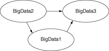
16. Directed graph representing a small part of the Web.

Each page has a PageRank indicating its importance or popularity. BigData3 will be the most highly ranked because it has the most links going to it, making it the most popular. Suppose now that a random surfer visits a webpage, he or she has one proportional vote to cast, which is divided equally between the next choices of webpage. For example, if our random surfer is currently visiting BigData1, the only choice is to then visit BigData3. So we can say that a vote of 1 is cast for BigData3 by BigData1.

In the real Web new links are made all the time, so suppose we now find that BigData3 links to BigData2, as shown in Figure 17, then the PageRank for BigData2 will have changed because the random surfer now has a choice of where to go after BigData3.

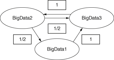
17. Directed graph representing a small part of the Web with added link.

If our random surfer starts off at BigData1, then the only choice is to visit BigData3 next and so the total vote of 1 goes to BigData3, and BigData2 gets a vote of 0. If he or she starts at BigData2 the vote is split equally between BigData3 and BigData1. Finally, if the random surfer starts at BigData3 his or her entire vote is cast for BigData2. These proportional ‘votes’ are summarized in the Figure 18.

18. Votes cast for each webpage.

Using Figure 18, we now see the total votes cast for each webpage as follows:

Total votes for BD1 are 1/2 (coming from BD2)

Total votes for BD2 are 1 (coming from BD3)

Total votes for BD3 are 1½ (coming from BD 1 and BD2)

Since the choice of starting page for the surfer is random, each one is equally likely and so is assigned an initial PageRank of 1/3. To form the desired PageRanks for our example, we need to update the initial PageRanks according to the proportion of votes cast for each page.

For example, BD1 has just 1/2 vote, cast by BD2, so the PageRank of BD1 is . Similarly, PageRank BD2 is given by and PageRank BD3 is . Since all the Page Rankings now add up to one, we have a probability distribution which shows the importance, or rank, of each page.

But there is a complication here. We said that the probability that a random surfer was on any page initially was 1/3. After one step, we have calculated the probability that a random surfer is on BD1 is 1/6. What about after two steps? Well, again we use the current PageRanks as votes to calculate the new PageRanks. The calculations are slightly different for this round because the current PageRanks are not equal but the method is the same, giving new PageRanks as follows: PageRank BD1 is 2/12, PageRank BD2 is 6/12, and PageRank BD3 is 4/12. These steps, or iterations, are repeated until the algorithm converges, meaning that the process continues like this until no more changes can be made by any further multiplication. Having achieved a final ranking, PageRank can select the page with the highest ranking for a given search.

Page and Brin, in their original research papers, presented an equation for calculating the PageRank which included a Damping Factor d, defined as the probability that a random Web surfer will click on one of the links on the current page. The probability that a random Web surfer will not click on one of the links on the current page is therefore , meaning that the random surfer has finished surfing. It was this Damping Factor that ensured the PageRank averaged over the entire Web settles down to 1, after a sufficient number of iterative calculations. Page and Brin reported that a web consisting of 322 million links settled down after fifty-two iterations.

Public datasets

There are many freely available big datasets that interested groups or individuals can use for their own projects. Common Crawl, mentioned earlier in this chapter, is one example. Hosted by the Amazon Public Datasets Program, in October 2016 the Common Crawl monthly archive contained more than 3.25 billion webpages. Public datasets are in a broad range of specialties, including genome data, satellite imagery, and worldwide news data. For those not likely to write their own code, Google’s Ngram Viewer provides an interesting way of exploring some big datasets interactively (see Further reading for details).

Big data paradigm

We have seen some of the ways in which big data can be useful and in Chapter 2 we talked about small data. For small data analysis, the scientific method is well-established and necessarily involves human interaction: someone comes up with an idea, formulates a hypothesis or model, and devises ways to test its predictions. Eminent statistician George Box wrote in 1978, ‘all models are wrong, but some are useful’. The point he makes is that statistical and scientific models in general do not provide exact representations of the world about us, but a good model can provide a useful picture on which to base predictions and draw conclusions confidently. However, as we have shown, when working with big data we do not follow this method. Instead we find that the machine, not the scientist, is predominant.

Writing in 1962, Thomas Kuhn described the concept of scientific revolutions, which follow long periods of normal science when an existing paradigm is developed and investigated to the full. If sufficiently intractable anomalies occur to undermine the existing theory, resulting in loss of confidence by researchers, then this is termed a ‘crisis’, and it is ultimately resolved by a new theory or paradigm. For a new paradigm to be accepted, it must answer some of the questions found to be problematic in the old paradigm. However, in general, a new paradigm does not completely overwhelm the previous one. For example, the shift from Newtonian mechanics to Einstein’s relativity theory changed the way science viewed the world, without making Newton’s laws obsolete: Newtonian mechanics now form a special case of the wider ranging relativity theory. Shifting from classical statistics to big data analytics also represents a significant change, and has many of the hallmarks of a paradigm shift. So techniques will inevitably need to be developed to deal with this new situation.

Consider the technique of finding correlations in data, which provides a means of prediction based on the strength of the relationships between variables. It is acknowledged in classical statistics that correlation does not imply causation. For example, a teacher may document both the number of student absences from lectures and student grades; and then, on finding an apparent correlation, he or she may use absences to predict grades. However, it would be incorrect to conclude that absences cause poor grades. We cannot know why the two variables are correlated just by looking at the blind calculations: maybe the less able students tend to miss class; maybe students who are absent due to sickness cannot later catch up. Human interaction and interpretation is needed in order to decide which correlations are useful.

With big data, using correlation creates additional problems. If we consider a massive dataset, algorithms can be written that, when applied, return a large number of spurious correlations that are totally independent of the views, opinions, or hypotheses of any human being. Problems arise with false correlations—for example, divorce rate and margarine consumption, which is just one of many spurious correlations reported in the media. We can see the absurdity of this correlation by applying scientific method. However, when the number of variables becomes large, the number of spurious correlations also increases. This is one of the main problems associated with trying to extract useful information from big data, because in doing so, as with mining big data, we are usually looking for patterns and correlations. As we will see in Chapter 5, one of the reasons Google Flu Trends failed in its predictions was because of these problems.