PROBLEM 3-1
Propositional proofs and truth tables allow us to prove things about relationships between whole sentences, but for some arguments we must break sentences down and see their internal structure—how the constituent parts of a proposition work together. To do this kind of proof rigorously, we can use predicate logic, also called the predicate calculus. Like the propositional calculus, it’s a formal system.
CHAPTER OBJECTIVES
In this chapter, you will
• Render complex sentences in symbolic form.
• Compare universal and existential quantifiers.
• Learn how quantifiers relate.
• Construct well-formed formulas.
• Work with two-part relations and syllogisms.
• Execute proofs in predicate logic.
In order to unambiguously construct statements and execute proofs that depend on internal sentence structure, we must introduce symbols that allow us to rigorously talk or write about them.
In formal logic, we represent predicates as capital letters of the alphabet called predicate letters. For example, we might write W for “walks” and J for “jumps.” As with the variables of propositional logic, we can choose any letter to stand for a predicate, but we must avoid using the same letter for two different predicates in a single proof, derivation, or argument. (Otherwise we’ll introduce ambiguity.)
We represent the subjects of sentences as italicized lowercase letters called subject letters. A noun or proper name constitutes a simple, and common, subject. For instance, we might translate the proper name “Jack” to the letter j and the noun “science” to the letter s. When possible, we’ll use the initial letter of the noun we want to symbolize, while making sure not to assign a particular letter more than once in a single proof, derivation, or argument.
Quite often, we’ll want to construct sentences with the noun “any given person” or “a certain triangle” instead of naming a particular person or thing. We call this type of noun an arbitrary name (or an arbitrary constant) and symbolize it with an italicized, lowercase letter, just as we do with specific subjects. By convention, we’ll start from the beginning of the alphabet (a, b, c, …) when assigning these symbols. We can refer to proper and arbitrary nouns generally as names, terms, or constants.
When we need a “placeholder” to stand for a constant in a proposition, we will use a logical variable, also known as an individual variable. (We’ll rarely run any risk of confusing it with a propositional variable, so we can simply call it a variable.) We symbolize variables, like names, with lowercase italicized letters. The traditional letter choices are x, y, and z—just like the letters that represent common variables in mathematics. If we need more letters for variables, we can also use u, v, and w.
To form a complete predicate statement, we can place a predicate letter next to a name or an individual variable, writing the predicate first. For example, if someone says “Roger eats beef,” we can write it as Er (with E symbolizing “eats beef” and r symbolizing “Roger”). We call this form an elementary sentence (also known as an atomic sentence or singular proposition), because it constitutes the simplest form for a complete statement in the predicate calculus.
TIP Even though they possess internal structures (unlike propositional variables), atomic sentences are the simplest elements in the formal system of predicate logic to which we can assign truth values.
PROBLEM 3-1
Translate the following sentences into formal predicate propositions using predicate letters and names:
• Jill has a cold.
• You will arrive late.
• Ruth lives in America.
• I walked.
 SOLUTION
We replicate the sentences below, along with letters assigned as their symbols and translated into predicate formulas. You might want to assign different letters to the names and predicates, but the complete statements should have the same form as the ones below, no matter what particular letters you choose:
• Jill (l) has a cold (C). Cl
• You (u) will arrive late (L). Lu
• Ruth (r) lives in America (A). Ar
• I (i) walked (W). Wi
Not every predicate formula contains a single predicate and a single constant (or stand-in variable). If we want to symbolize “Jack walks to work” and “Ruth walks home,” we could simply write Kj and Nr, but we can’t see from this two-part structure that both Jack and Ruth are walking (as opposed to, say, running, riding bicycles, or driving cars). In order to symbolize this level of structural detail, we need a type of predicate called a relation. Relations apply to more than one constant (or variable), and they allow us to express a relationship between two things (instead of a property of only one thing). For this reason, logicians sometimes refer to relations as dyadic (two-part) and polyadic (many-part) predicates.
We can analyze sentences of this more complicated sort as relations with constants symbolizing both the subject of the sentence (Jack or Ruth) and the destination (school or home, respectively). To write a relation as a formula, we use a predicate letter followed by two names. For example, we might symbolize “Jack walks to school” and “Ruth walks to her house” as Wjs and Wrh, respectively, where W stands for “—walks to—.” We can see from these formulas that the predicate has the same form in both cases, suggesting the analogy “j is to s as r is to h” (even if we don’t know what the symbols stand for). Note that when we put more than one constant into a formula with a predicate letter, we must make sure that we put the symbols in the correct order. We don’t want to end up with a formula that says “School walks to Jack!”
Most predicates that you’ll likely see constitute one-place properties or two-place relations. But in theory, a predicate can take any finite number of constants. For example, we could make a three-place relation (using the letter assignments we established before for the names), symbolizing “Jack and Ruth are Jill’s parents” by writing Pjrl.
TIP Occasionally, we’ll encounter a predicate that doesn’t apply to any names at all. In a situation like this, we have an atomic sentence consisting of one predicate letter by itself; the resulting proposition constitutes an atomic propositional variable, and we can symbolize it the same way as we do in the propositional calculus (as a capital letter). We can consider a predicate accompanied by any finite number of names to constitute an atomic sentence, as long as we have the correct number of names for that specific predicate.
One important type of basic sentence is an assertion of identity. Propositions of this sort say that two names go with the same object, or that they’re equivalent to one another. Sentences such as “Ruth is the boss,” “I am the one who called,” and “Istanbul is the same city as Constantinople” constitute statements of identity.
In formal logic, we can think of identity as a two-place relation. Because of its special importance, we symbolize it with an equals sign (=) instead of a predicate letter. The identity symbol goes between the two names that we want to identify, and parentheses go around the three symbols. Using this notation, we could translate “I am Jack” to (i = j), or “Science is my favorite subject” to (s = f).
When we identify two nouns with each other, we can interchange them without affecting the truth value of the whole. If we know that “Jack is Mr. Doe,” then we can replace “Jack” with “Mr. Doe” in any sentence where we find it without changing its truth value. All the same predicates and logical relationships apply to the two names, because both names refer to the same man!
Once we have a collection of complete predicate sentences, we can modify them and show their logical relationships. In order to do this, let’s carry over all of the operators established for the propositional calculus in Chap. 2, along with their symbols, as follows:
• Negation (¬)
• Conjunction (∧)
• Disjunction (∨)
• Implication (→)
• Biconditional (↔)
All the rules concerning the order of operations in propositional logic, including the use of parentheses, apply to predicate logic as well. When we start working out predicate proofs, therefore, we’ll be able to use all of the propositional inference rules for the operators.
Translate the following sentences into formal predicate propositions using predicate letters, names, and the logical operators:
• You will be late, but I will not be late. (Note that “but” means the same thing as “and” in this context.)
• Jill and Roger are siblings. (Symbolize both “Jill” and “Roger” as proper names.)
• If Jack isn’t walking, then he must be jumping.
• My grandfather is the person wearing orange. (Use two proper names.)
• My dog is well-trained and obedient, or she is not well-trained and unruly.
SOLUTION
• You (u) will be late (L), but I (i) will not be late. Lu ∧ ¬Li
• Jill (l) and Roger (r) are siblings (S). S/r
• If Jack (j) isn’t walking (W), then he must be jumping (J). ¬Wj → Jj
• My grandfather (g) is the person wearing orange (o). (g = o)
• My dog (d) is well-trained (B) and obedient (V), or she is not well-trained and unruly (U). (Bd ∧ Vd) ∨ (¬Bd ∧ Ud)
Using predicate letters, names, and logical operators, we can carry out all the same sorts of proofs with predicate sentences that we can do in the propositional calculus. We must go further than that, however, to take advantage of the internal structure shown by predicate propositions. To argue effectively about applying predicates to names, we can “quantify” our statements so we can talk about sets of objects like “everything that has the property F,” “no two things that are in relation G to each other,” or “some of the things that are both F and H.” This methodology allows us to prove sequents about predicates and names in general.
Suppose you tell your friend that “Some dogs are terriers.” You have two predicates to consider: the property of being a dog (call it D) and the property of being a terrier (T). To interpret this statement as a logical proposition, think of the evidence you need to know its truth value. A single example of an object that’s both a dog and a terrier will demonstrate the validity of your statement. Therefore, the statement “Some dogs are terriers” is equivalent to “There’s at least one thing that is both a dog and a terrier” or “Something exists that is both a dog and a terrier.” (In common speech, “some” often means “more than one,” but for our purposes it means “at least one.”) Using a singular variable, x, to represent “a thing” or “something” in the formula, you can say that there exists an x that makes the conjunction Dx ∧ Tx true.
Now imagine that your friend says “All dogs are mammals.” Once again, you have two predicate properties. You might symbolize the property of being a mammal with the letter M. The logical interpretation of your friend’s statement transforms it into a conditional proposition: “It is true of everything that if it is a dog, then it is a mammal” or “If something is a dog, then it is a mammal.” These two statements have equivalent meaning, even though you might find that fact difficult to comprehend at first thought. (The statements both hold true under exactly the same conditions; in order to prove either statement false, we’d have to find a dog that’s not a mammal.) Using an individual variable to translate the word “something,” you can say that for anything whatsoever (represented by the variable x), Dx → Mx.
When we translated the sentence “Some dogs are terriers” into symbols above, we left one part in ordinary language: “There exists an x.” We can’t leave this part out! The formal predicate language must adhere to strict rules. We call the “there is” or “there exists” portion of the proposition the existential quantifier, and its symbol looks like a backward capital letter E (∃).
We can read the existential quantifier out loud as “There is…” or “There exists…” or “For some…” We always follow it with a variable, and then place the character sequence in parentheses. For example, (∃x) means “There is an x” or “There exists an x” or “For some x.” In a situation of this sort, we “quantify over” the variable that accompanies the ∃ symbol. For example, we might place (∃x) at the beginning of a formula, and then follow that quantifier with a proposition built up from predicate sentences that include the variable x. When fully expressed by symbols, the sentence “Some dogs are terriers” translates symbolically to
[∃x] Dx ∧ Tx
If we read the above formula out loud, we say “There exists an x such that Dx and Mx.” Fully translating, and letting D represent “is a dog” and T represent “is a terrier,” we get “There exists an object x such that x is a dog and x is a terrier.” This statement constitutes an example of an existentially quantified proposition. Some texts might call it an existential statement or a particular sentence.
We also need a symbol to stand for “For all…” or “For every…” (as in the formula for “All dogs are mammals” above). We call this symbol the universal quantifier. It looks like an upside-down capital letter A (∀). As with the existential quantifier, we need to “quantify over” a variable, and we use the same general syntax. We write the variable symbol immediately after the quantifier, enclosing both symbols in parentheses, usually at the beginning of a proposition. [Some texts place a variable alone within parenthesis to represent universal quantification, for example (x) rather than (∀x).] According to the convention that we will use, the plain-language sentence “All dogs are mammals” translates to the symbol sequence
(∀x) Dx → Mx
Reading the above formula out loud, we say “For all x, if Dx, then Mx.” Fully translating, we obtain the sentence “For all objects x, if x is a dog, then x is a mammal.” This statement demonstrates an example of a universally quantified proposition (also known as a universal statement or general sentence).
In order to know that a simple existential statement holds true, you need to produce only one example of the property or properties attributed to the variable. The example might be “definite,” using a proper noun, or “arbitrary,” with an arbitrary name. If you want to ensure that a universal statement holds true, however, you must demonstrate that it holds true for every possible example. A single counterexample will invalidate it, no matter how many examples make it seem true. In fact, a single counterexample will invalidate a statement for which infinitely many other examples work!
What counts as “every possible example” depends on the context. If we discuss siblings, then “every possible example” might constitute the set of all humans (a large but finite set). If we talk about mathematics, then “every possible example” might constitute the set of all real numbers (an infinite set). We call such a set the universe of discourse or simply the universe; some texts call it the domain of discourse. In many cases, we can take for granted the sorts of objects to which a predicate can apply; in other situations we must define the universe explicitly (especially when using quantifiers).
Thinking about and clearly defining the universe can help make sense of some quantified statements. We can imagine the existential quantifier as a long disjunction. For example, the formula
(∃x) Fx
is like the long disjunction
Fm ∨ Fn ∨ Fo …
where the set {m, n, o,…}, the universe, contains every object—but only those objects—to which the predicate might apply. If any of the disjuncts is true, then the predicate is true of something; a single example is all we need to demonstrate the validity of the statement. We can refer to the corresponding arbitrary statement Fa as the typical disjunct or representative instance of (∃x) Fx, because it can stand for any element of the set of statements {Fm, Fn, Fo,…}.
Following along similar lines, we can imagine the universal quantifier as a long conjunction; the formula
(∀x) Fx
is like the long conjunction
Fm ∧ Fn ∧ Fo ∧ …
where the set {m, n, o, …}, the universe, contains every object—but only those objects—to which the predicate might apply. The whole conjunction holds true if and only if every conjunct is true; if only one of the conjuncts is false, then the whole conjunction is false. We can refer to the arbitrary statement Fa as the typical conjunct or representative instance of (∀x) Fx, because it can stand for any element of the set {Fm, Fn, Fo, …}.
TIP The universe may contain a finite number of things, but in many instances we’ll encounter universes that contain infinitely many elements (the set of all positive whole numbers or the set of all real numbers, for instance). In a situation like that, we can’t write out a quantifier’s equivalent conjunction or disjunction completely, but we can nevertheless use this device as a way of thinking about the truth conditions of quantified propositions. In this book, we’ll always assume that the universe contains at least one element. We won’t get into the esoteric business of ruminating over empty universes!
A single sentence can have more than one quantifier, each applying to a different variable. For instance, you might say, “Some people have a sibling.” To express this sentence symbolically using the sibling relation S, we need two existential quantifiers (one for “some people” and one for their unnamed siblings), producing the formula
[∃x)(∃y) Sxy
When all the quantifiers in a multiple-quantifier formula are of the same type (universal or existential, as in this example), then we can list the quantifier once, with all the applicable variables listed immediately to its right, obtaining
(∃x, y) Sxy
We would read this out loud as “There exist an x and a y such that Sxy.”
When using multiple variables and quantifiers, we must always assign a unique variable to each constant in a formula. In the foregoing situation, we wouldn’t want to write a formula such as
(∃z) Szz
which, translated literally, means “There exists a z who is his or her own sibling.”
If we want to construct a proposition that requires both a universal quantifier and an existential quantifier, we must preserve the orders of the quantifiers and variable assignments. Otherwise, we might commit the “fallacy of every and all,” an example of which is
(∀y)(∃x) Rxy
If we let R mean “is an ancestor of,” then this formula translates to “Everyone has somebody else as an ancestor.” It’s obviously not equivalent to
(∃x)(∀y) Rxy
which translates to “There is someone who is an ancestor of everybody else.”
PROBLEM 3-3
Translate the following English sentences into formal predicate propositions using quantifiers and variables (use x) in addition to the other symbols you’ve learned:
• All dogs are well-trained.
• Somebody is Jack’s sibling. (Use a two-part relation.)
• Some Americans have colds.
• For any pair of siblings, one is older than the other.
• Everybody was late.
SOLUTION
You can assign predicates and variables, and then break down the sentences into formal predicate propositions as follows:
• All dogs (D) are well-trained (B). (∀x)Dx → Bx
• Somebody is Jack’s (j) sibling (S). (∃x) Sxj
• Some Americans (A) have colds (C). (∃x)Ax ∧ Cx
• For any pair of siblings (S), one is older(O) than the other. (∀x, y) Sxy → Oxy ∨ Oyx
• Everybody was late (L). (∀x) Lx
These are the most straightforward, recognizable ways to symbolize these sentences. We can make up plenty of other, logically equivalent formulas that hold true under the same conditions.
Subtle distinctions occur when we translate the existential quantifier to the universal, or vice versa. When we want to assert a combination of properties, the existential quantifier employs conjunction, while we express universal statements using the conditional (if/then) operator. For example, “Some Americans have colds” translates to
(∃x) Ax ∧ Cx
but “All Americans have colds” translates to
(∀x) Ax → Cx
We must use the applicable connecting operator (∧ with ∃ and → with ∀), or we might lose the meaning in translation. For example, if we write
(∀x) Ax ∧ Cx
using the above assignments, we say, in effect, that “Everyone is an American with a cold.” That wouldn’t hold true even if everybody in the world had a cold!
We can transform any quantified statement from universal to existential or vice versa using the negation operator. For instance, the universal sentence “Everybody was late,” symbolized as
(∀x) Lx
means the same things as the existential sentence “There was nobody who was not late,” which we symbolize as
¬(∃x) ¬Lx
The negation of the first statement, “Not everyone was late,” symbolized as
¬(∀x) Lx
holds true under the same conditions as the negation of the second statement, “Someone was not late,” symbolized as
(∃x) ¬Lx
We can state two general equivalences of this kind, called the laws of quantifier transformation. (These rules might remind you of DeMorgan’s laws, which transform between conjunction and disjunction using negation.) They show that the quantifiers are interderivable, meaning that we can reformulate any quantified statement in terms of a single quantifier (either universal or existential). We express the laws of quantifier transformation as
(∃x) Fx  ¬(∀x ¬Fx
and
(∀x) Fx ¬(∃x ¬Fx
Both propositions in either transformation have the same truth value, so their negations must have the same truth value, too. By negating both sides of the equivalence sequents and eliminating double negation, we can see the laws in the forms
¬(∃x) Fx (∀x ¬Fx
and
¬(∀x) Fx (∃x ¬Fx
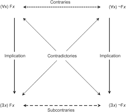
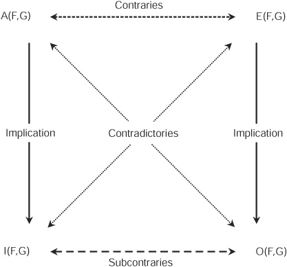
The logical relationships between quantified statements can be summed up in a diagram called a square of opposition (Fig. 3-1). Propositions located at opposite corners contradict (they negate each other). The universal propositions on top imply the existential propositions directly below them; if a property applies to everything, then it applies to something. We call the universal statements on the top of the square contraries (they never hold true at the same time, but might both be false) and the existential statements on the bottom of the square subcontraries (they are never both false, but both may hold true).
Figure 3-1 · The square of opposition for logical quantifiers.
If we want to ensure that our formulas express genuine propositions in predicate logic, we need a set of rules against which we can test them. If a formula follows the rules, we call it a well-formed formula (WFF). The following rules define the sorts of formulas that qualify as WFFs in predicate logic.
• Any PF (as defined in Chap. 2) constitutes a WFF.
• Any subject/predicate formula in which a predicate letter is followed by a finite number of terms, such as Ak, constitutes an atomic sentence, and all atomic sentences are WFFs. For example, if A is a predicate and k is a constant, then Ak is a WFF; if k1 k2, k3,…kn are constants, then Ak1k2…kn is a WFF. (For a propositional variable, n = 0.) Identity is a special predicate relation, and the identity symbol is analogous to a predicate letter. An identity statement like (k1 = k2), written inside parentheses, constitutes an atomic sentence. For example, if k1 and k2 are constants, then (k1 = k2) is a WFF.
• Any WFF immediately preceded by the symbol ¬, with the whole thing inside parentheses, is a WFF. For example, if X is a WFF, then (¬X) is a WFF.
• Any WFF joined to another WFF by one of the binary connectives ∧, ∨, →, or ↔, with the whole thing written inside parentheses, is a WFF. For example, if X is a WFF, Y is a WFF, and # is a binary connective, then (X # Y) is a WFF.
• If we replace a constant in a WFF consistently by a variable, this action constitutes a substitution instance of the WFF. If we place a quantifier and a variable in parentheses to the left of a substitution instance, the result is a WFF. For example, if X is a WFF including a constant k, @ is a quantifier, and Y is a substitution instance of X (the formula resulting when every instance of k in X is replaced by a variable v), then (@v) Y is a WFF.
• Any formula that does not satisfy one or more of the five conditions listed above does not constitute a WFF.
You can drop some of the parentheses from your formulas according to the conventional order of operations. We did that in some of the examples above; for example, the rigorous form of
(Bd ∧ Vd) ∨ (¬Bd ∧ Ud)
would be written as
{(Bd ∧ Vd) ∨ [(¬Bd] ∧ Ud]}
with two extra sets of grouping symbols. You can drop the extra grouping symbols to make WFFs easier to read, but you can substitute them back in at any time to satisfy the strict definition of a WFF above, or whenever doing so makes a formula easier for you to understand.
TIP A statement can form a legitimate WFF even if it doesn’t hold true. Statements whose truth value remains unknown, and even statements that are obviously false, can constitute perfectly good WFFs! They only need to follow the foregoing rules concerning the arrangements of the symbols.
Two-part predicates have a set of logical categories all their own, called the properties of relations. Let’s define the most important general properties.
A relation is symmetric if it makes the following proposition true whenever we substitute it for F in the formula
(∀x, y) Fxy → Fyx
This rule tells us that we can always transpose or rearrange the order of the variables or constants without changing the truth value. The property of “being a sibling,” for example, is a symmetric relation. If Jill is Roger’s sibling, then Roger is Jill’s sibling. Identity is also symmetric: if x = y, then y = x. Because we state the rule universally, one counterexample will demonstrate that a relation is not symmetric.
If a relation holds true in one “direction” but not the other, we call that relation asymmetric. Using the same symbol convention as we did when we stated the criterion for symmetry, we can express the criterion for asymmetry as
(∀x, y) Fxy → ¬Fyx
The property of “being older than someone” is asymmetric. If Jill is older than Roger, then Roger is not older than Jill. If we can find one case where the order of names doesn’t affect the proposition truth value of the proposition Fxy, then we’ve proved that F isn’t asymmetric.
Sometimes a predicate follows the rule of asymmetry except when we use the same name twice. Consider the mathematical relations “less than or equal to” (≤) and “greater than or equal to” (≥). The asymmetry rule holds true of these relations for most numbers we can assign to x and y, but not when we choose the same number for both variables. We call this type of relation antisymmetric, and we can express the criterion as
(∀x, y) Fxy ∧ Fyx → (x = y)
A relation that’s neither symmetric nor antisymmetric (and therefore not asymmetric, either) is known as nonsymmetric. Now we’ve covered everything!
TIP We can always put any given relation in the predicate calculus into one or more of the above-defined four categories of symmetry.
If a predicate relation holds between any name and itself, then we call that relation reflexive. For example, the following relation exhibits reflexivity:
(∀x) Fxx
We need not work very hard to come up with specific cases of reflexivity. Everything is identical to itself, every woman is the same age as herself, and so on. If we can come up with a single example of a constant where the predicate does not hold true in this way, then the relation is not reflexive.
If a relation cannot hold between any constant and itself, like the property of being older than someone, then we call that relation irreflexive. We can define this property by writing the relation
(∀x) ¬Fxx
If some substitution instances make Fxx true and others make ¬Fxx true, then the relation F does not meet the definition for reflexivity or irreflexivity. In a case of this sort, we categorize the relation as nonreflexive.
TIP Any given relation will satisfy only one of the foregoing three criteria; it must be either reflexive, irreflexive, or nonreflexive.
Suppose we have a relation that holds true between x and y and also between y and z. We call that relation transitive if it also holds true between x and z. We can define transitivity in symbolic terms as
(∀x, y, z) F xy ∧ Fyz → Fxz
The relation of “being older” provides us with an example of transitivity. If Ruth is older than Jill and Jill is older than Roger, then we know that Ruth must be older than Roger. Identity also constitutes a transitive relation. Can you think of others?
Any case that contradicts the universal proposition above indicates that transitivity does not hold for the relation in question; when no examples show this pattern, we call the relation intransitive. We can define intransitivity in symbolic terms as
(∀x, y, z) Fxy ∧ Fyz → ¬Fxz
For instance, if Tuesday is the day immediately before Wednesday, and Wednesday is the day immediately before Thursday, then Tuesday can’t be the day immediately before Thursday.
If a relation meets neither of the preceding two criteria, then we call it nontransitive. For this type of relation, we could produce counterexamples to the universal statements that express transitivity and intransitivity.
TIP Any given two-part relation will satisfy only one of the foregoing three criteria; it must be either transitive, intratransitive, or nontransitive.
We can always describe a two-part predicate relation, no matter how complicated or esoteric, in terms of the symmetry, reflexivity, and transitivity criteria and their variants. If a relation meets the criteria for symmetry, reflexivity, and transitivity “all at the same time,” then we call it an equivalence relation. We have established that identity, an especially important relation in logic, constitutes an equivalence relation.
With the symbols of the predicate calculus we can make rigorous arguments that take advantage of sentence structure. All of the proof methods, inference rules, and laws that we learned in propositional logic still apply, but predicate proofs require us to adopt some new inference rules.
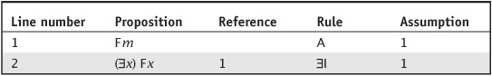
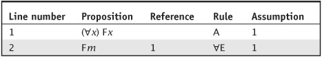
A single instance of a predicate applied to a constant can serve as a premise to derive an existential statement about a variable. We replace the constant consistently using the same variable that goes next to the quantifier. (We should, of course, choose a new variable letter that we haven’t used elsewhere in the proof.) We call this principle the rule of existential introduction; we can symbolize it as ∃I. To implement it during the course of a proof, we cite the atomic sentence in the reference column and carry over its assumptions, as shown in Table 3-1.
TABLE 3-1 An example of existential introduction.
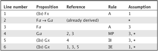
We can derive conclusions using an existential statement as a premise by invoking the rule of existential elimination. If we can prove the desired conclusion using an “arbitrary example” of a property (that is, an atomic sentence that includes an arbitrary name) assumed as a premise, then we can derive the same conclusion from a statement that says something with that property exists. The assumed premise should look like the existential proposition, but with the quantifier dropped and the arbitrary name consistently replacing the existentially quantified variable.
To take advantage of this rule, we need to reference three lines: the arbitrary sentence used as a premise, the statement proved from it, and the existential premise. From the assumptions listed with the first statement of the conclusion, we drop the assumption corresponding to the arbitrary premise and replace it with the assumption(s) of the existential statement. (This procedure may remind you of disjunction elimination; we derive a conclusion and then “swap out” the assumptions.) In the rule column, we write ∃E.
The arbitrary name constitutes a temporary device in this kind of derivation, used as a typical disjunct for the existential proposition. We must treat it carefully in order to avoid generating a fallacious argument. In the final step, where we apply ∃E, we drop the assumption involving the arbitrary name. To ensure a valid deduction, that arbitrary name should not appear in the conclusion itself or in any of the remaining assumptions.
TABLE 3-2 An example of existential elimination.
The example in Table 3-2 starts off “in the middle,” as if we had already proved the arbitrary sentence at line 2, Fa → Ga, on the basis of some unknown assumptions signified by an asterisk (*). We can assume that no proposition in * includes the arbitrary name a. Doing that keeps the proof simple without violating the restriction on assuming a proposition with arbitrary name.
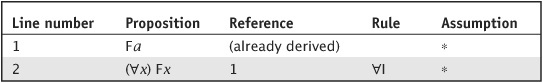
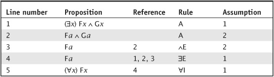
In an atomic proposition with an arbitrary name such as Fa where the arbitrary name stands for “anything”; we can understand the statement to mean “Take anything you like; that thing has property F.” If property F applies to anything that we might happen to pick out, then we can conclude that F must apply to everything. We call this principle the rule of universal introduction, abbreviated ∀I. When employing this rule, the arbitrary statement is the only premise referenced, and all of its assumptions are retained.
Whenever we invoke ∀I, the arbitrary name should not appear in any of the assumptions cited alongside the conclusion. The conclusion itself constitutes a universally quantified proposition with every appearance of the arbitrary name replaced by the quantified variable.
Table 3-3 begins with the typical conjunct Fa, as if we had already derived it from a set of assumptions signified by an asterisk (*). We can assume that no proposition in * includes the arbitrary name a. Making this assumption keeps the proof as simple as possible without violating the restriction on assuming a proposition with an arbitrary name.
TABLE 3-3 An example of universal introduction.
A universal statement holds true only if every single atomic sentence we can produce from it is true, so we can use the general statement as a premise to derive one of its instances. To take advantage of the rule of universal elimination, we reference the universal as a premise, carry over its assumptions, and fill in any constant we like, consistently substituted in place of the universally quantified variable. In the rule column, we write VE as shown in Table 3-4.
TABLE 3-4 An example of universal elimination.
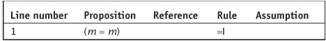
When we want to bring a statement of identity into a proof, we can use the rule of identity introduction. This inference rule derives from the trivial reasoning that any name is self-identical (everything is itself!). We can always substitute a name for itself without changing the truth value of a proposition, because the resulting formula looks exactly the same as it did before. Using identity introduction, we can introduce a proposition of the form (m = m) at any point in a proof without having to cite any premises or assumptions whatsoever. We write =I in the rule column to indicate the use of this rule, as shown in Table 3-5.
TABLE 3-5 An example of identity introduction.
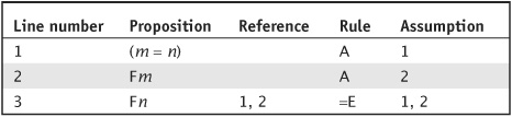
TABLE 3-6 An example of identity elimination.
If two names are identical, then we can substitute one for another. This principle is the basis for the rule of identity elimination, symbolized =E. To use the rule, we reference two lines as premises: an identity statement and another proposition including one (or both) of the identified names. Then we can derive a substitution instance of the target proposition, “swapping out” one name for another. We don’t have to substitute all instances consistently; we can choose at will between the names in each instance where one of them appears, and finally combine the assumptions of the two premises. Table 3-6 illustrates how =E works.
In predicate proofs, we can quantify the assumptions and conclusions (propositions appearing in the proved sequent) to keep arbitrary constants out of sequents. As the restrictions on universal introduction and existential elimination suggest, we should strive to use arbitrary names only on a temporary basis. We can “extract” them from quantified statements using the quantifier inference rules, manipulate the resulting arbitrary atomic sentences with propositional transformations, and then “requantify,” substituting all the arbitrary constants with quantified variables in the conclusion.
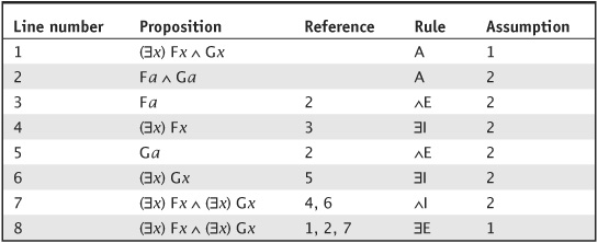
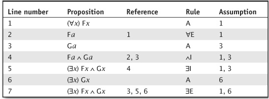
PROBLEM 3-4
Use the inference rules to prove the sequent
(∃x) Fx ∧ Gx  (∃x) Fx ∧ (∃x) Gx
SOLUTION
See Table 3-7.
TABLE 3-7 Proof that (∃x) Fx ∧ Gx (∃x) Fx ∧ (∃x) Gx.
PROBLEM 3-5
Use the inference rules to prove the sequent
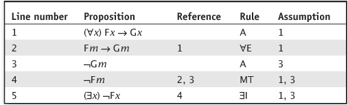
(∀x) Fx → Gx, ¬Gm (∃x) ¬Fx
SOLUTION
See Table 3-8.
PROBLEM 3-6
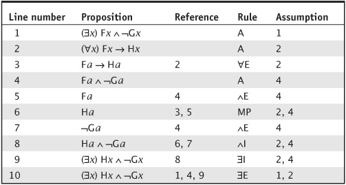
Use the inference rules to prove the sequent
(∃x) Fx ∧ ¬Gx, (∀x) Fx → Hx (∃x) Hx ∧ ¬Gx
SOLUTION
See Table 3-9.
TABLE 3-8 Proof that (∀x) Fx → Gx, ¬Gm (∃x) ¬Fx.
TABLE 3-9 Proof that (∃x) Fx ∧ ¬Gx, (∀x) Fx → Hx (∃x) Hx ∧ ¬Gx.
PROBLEM 3-7
Use the inference rules to prove the sequent
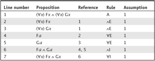
(∀x) Fx ∧ (∀x) Gx (∀x) Fx ∧ Gx
SOLUTION
See Table 3-10.
TABLE 3-10 Proof that (∀x) Fx ∧ (∀x) Gx (∀x) Fx∧ Gx.
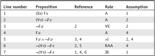
Use the inference rules to prove the laws of quantifier transformation
(∃x) Fx ¬(∀x) ¬Fx
and
(∀x) Fx ¬(∃x) ¬Fx
SOLUTION
Both laws constitute interderivability sequents, so we must execute a total of four proofs to back them up. Tables 3-11 through 3-14 show the derivations.
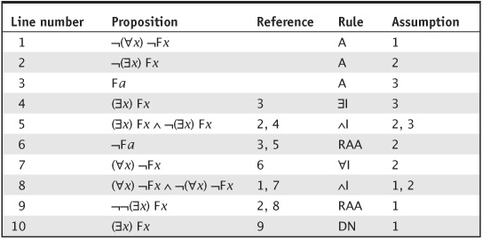
TABLE 3-11 Proof that (∃x) Fx ¬(∀x) ¬Fx.
TABLE 3-12 Proof that ¬(∀x) ¬Fx (∃x) Fx.
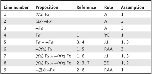
TABLE 3-13 Proof that(∀x) Fx ¬(∃x) ¬Fx.
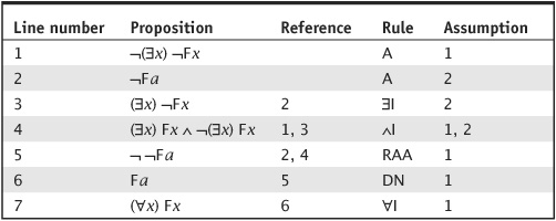
TABLE 3-14 Proof that ¬(∃x) ¬Fx (∀x) Fx.
The term syllogism refers to a well-known argument form in three lines with an alternate symbolism. We can use a syllogism as an abbreviated way to do certain predicate proofs. Syllogistic arguments constitute a subset of all possible predicate arguments. Not all predicate proofs can be expressed as syllogisms, and not all WFFs of the predicate calculus can appear in a syllogism, but all syllogisms can be expressed in the formal predicate system (if we follow some restrictions) and proved according to the conventional rules.
The following proof, expressed in everyday language, gives us a simple example of a syllogism:
All dogs are mammals.
All terriers are dogs.
Therefore, all terriers are mammals.
This argument is a traditional syllogism (also called a categorical syllogism), which means that it has three lines; each of the three propositions is quantified and contains two predicates.
We will find four types of proposition used in a traditional syllogism. We call such propositions categorical statements, and they have their own symbolism.
A universal affirmative proposition (abbreviated A) has the form
(∀x) Fx → ¬Gx
like the statement “All dogs are mammals.” In syllogistic notation, we denote this form as
A(F, G)
A universal negative proposition (E) has the form
(∀x) Fx → ¬Gx
like the statement “Anything that is an insect cannot be a mammal.” In syllogistic notation, we denote this form as
E(F, G)
A particular affirmative proposition (I), has the form
(∃x) Fx ∧ Gx
like the statement “There is at least one dog that is a mammal.” In syllogistic notation, we denote this form as
I(F, G)
A particular negative proposition (O) has the form
(∃x) Fx ∧ ¬Gx
like the statement “Some fish are not mammals.” In syllogistic notation, we denote this form as
O (F,G)
The WFF equivalents of the four proposition types are all quantified over a single variable.
The three-line argument stated a while ago (concerning dogs and mammals), rewritten in syllogistic notation, consists entirely of universal affirmatives. The original syllogism (in words) appears on the left below, while the symbolic version appears on the right. Let D = dog, M = mammal, and T = terrier. Then we can write
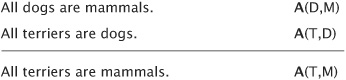
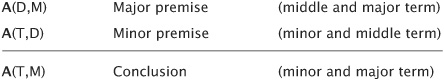
In a syllogism, we call the letters representing predicates the terms. (We must take care to avoid confusing syllogistic terms with proper or arbitrary names, also sometimes referred to as “terms” when they don’t appear in syllogisms.) We can call the first term the subject term and the second term the predicate term, corresponding to the “subject/predicate” order that we commonly use in everyday speech.
Every complete syllogism involves three terms. The major term appears in the first premise and the conclusion; in the above example, M constitutes the major term. The minor term is used in the second premise and the conclusion, like T in the above sample argument. The middle term always occurs in both premises, but not in the conclusion; D fills this role in the above argument. On the basis of the terms they include, we call the premises the major premise (the first) and the minor premise (the second). Therefore, we can generalize the above argument as follows:
These rules help us to simplify formal syllogisms, but they don’t encompass every possibility. Syllogisms in everyday speech might deviate from these conventions and nevertheless produce valid arguments.
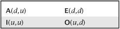
TIP We call a term distributed if it refers to everything with that property as used in the proposition. If we know the proposition type and position of the term (first or second in the statement), then the distribution appears as shown in Table 3-15 (with d for distributed, u for undistributed).
TABLE 3-15 Distribution of terms.
We can reverse the order of the terms in the universal negative (E) and the particular affirmative (I) forms without changing the truth value. Two laws summarize these allowed reversals: the law of the conversion of E and the law of the conversion of I. We can state them symbolically as
E(F, G) ↔ E(G, F)
and
I(F, G) ↔ I(G, F)
Because the rules governing syllogistic form are strictly limited (three lines and four proposition types), only a finite number of possible argument patterns can constitute well-formed syllogisms. We can classify well-formed syllogisms according to the pattern of the propositions (called the mood) and the arrangement of terms within the propositions (called the figure).
We define the mood of a syllogism according to the three proposition types that appear along the left side of the argument; we can name them using the three letters in the order they appear. The mood of the foregoing sample argument is AAA. There are four possible types of proposition for each line of the syllogism, which makes for 64 possible moods (4 × 4 × 4 = 43 = 64).
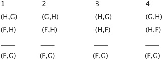
We define the figure of a syllogism as the four possible arrangements of terms (if we ignore the proposition types). If we call the minor term F, the major term G, and the middle term H, the four figures in the foregoing syllogism are as follows:
If we know both the mood and the figure of a syllogism, then we can uniquely define the logical form of the syllogism. The actual terms used to fill in the blanks are not logically important. Any of the four figures can be combined with any of the 64 moods, giving us a total of 256 possible patterns (4 × 64 = 256). We can identify any specific pattern by writing out the mood followed by the figure. The foregoing sample argument has the pattern of the first figure, so we can call it AAA1.
We can test the validity of syllogisms using any of several different techniques. Specialized diagrams known as Venn diagrams, adapted from set theory in pure mathematics, provide a powerful tool for this purpose. When used for syllogism-testing, a Venn diagram contains three circles, one for each term. We represent both premises on the same diagram. If the resulting picture illustrates the conclusion, then we know that we have a valid argument.
Figure 3-2 · A Venn interpretation of the syllogism AAA1. at a, the initial diagram, with mutually intersecting empty circles for d (dogs), M (mammals), and t (terriers). At B, the illustration for A (D, M), “All dogs are mammals.” At C, we add the illustration for A (T, D), “all terriers are dogs,” obtaining the conclusion A (T, M), “all terriers are mammals.”
To draw the diagram for AAA1 as it appears in the foregoing example, we start with three white circles, intersecting as shown in Fig. 3-2A. Then we shade or hatch (to eliminate) the region within the “dogs” (D) circle that does not intersect with “mammals” (M) to represent the first premise, A(D, M), as illustrated in Fig 3-2B. Next, for A(T, D), we shade or hatch (to eliminate) the region within the “terriers” (T) circle that does not intersect with “dogs” (D) on the same picture (Fig. 3-2C). To express the conclusion of the argument, A(T, M), we must shade or hatch the region within the “terriers” (T) circle that does not intersect with the “mammals” (M) circle—but we’ve already done that! The premises in combination determine the conclusion, so we know that our syllogism is valid.
We can also test a syllogistic argument using a set of principles intended to avoid fallacies. A formal syllogism, constructed according to the formation rules we’ve learned in this chapter, is valid if it satisfies the following conditions:
• At least one of the premises is affirmative (type A or I).
• If one premise is negative (type E or O), the conclusion must also be negative.
• If a term is distributed in the conclusion, it must also be distributed in the premise.
• The middle term must be distributed in at least one of the premises.
Some logicians draw a so-called square of opposition that shows the logical relationships between the syllogistic proposition types (Fig. 3-3). To ensure that these logical relationships to hold true, we must make some existential assumptions. Some of these logical relationships have existential import, which means that they do not hold if we fill in an “empty term” where the predicate does not apply to anything in the universe of discourse. (Traditional syllogisms assume that all terms must apply to something.) When looking at the diagram, we assume that no empty terms will exist. To demonstrate one of these relationships using a predicate proof, we may need to make an extra assumption of the form (∃x) Fx.
Figure 3-3 · The traditional square of opposition for categorical propositions.
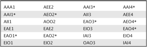
Only 24 of the 256 possible syllogisms constitute valid arguments (six per figure), as shown in Table 3-16.
The valid forms of syllogism have traditional nicknames according to their mood. Our example goes by the most famous of these names, “BARBARA.” The names give us a mnemonic device where the vowels spell out the mood; so, for example, BARBARA means the valid form of AAA (the one using the first figure, AAA1).
The starred forms in Table 3-16 have existential import, so each contains a “hidden” existential assumption about one of its predicates.
TABLE 3-16 Syllogisms that constitute valid arguments. Starred items have existential import.
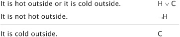
Not all syllogisms follow the traditional rules of form. For example, we can summarize propositional deductions in only three lines. Consider the following disjunctive syllogism:
A hypothetical syllogism resembles a modus ponens inference. We can represent this type of syllogism in three lines as well. For example:
You may refer to the text in this chapter while taking this quiz. A good score is at least 8 correct. Answers are in the back of the book.
1. If you know that Jack is American, the rule of existential introduction allows you to conclude that
A. somebody is American.
B. everyone (in the universe of discourse) is American.
C. an equivalent statement is “One American is Jack.”
D. for any given thing, if that thing is Jack, then it is American.
2. Which of the following formulas represents a good translation of the sentence “No mammals with colds are dogs”?
I. (∀x) Mx ∧ Cx → ¬Dx
II. (∀x) Dx → ¬Mx ∧ Cx
III. (∀x) (∃y) Mx ∧ Cx ∧ Dy
IV. (∃x) Dx → ¬(∀y) My ∧ Cy
V. ¬(∃x) Mx ∧ Cx ∧ Dx
A. I, II, and IV
B. only II
C. I and V
D. None of the above
3. Of the four quantifier inference rules (∃I, ∃E, ∀I, and ∀E), which involves dropping an assumption from the premises?
A. ∃I and ∃E (but not ∀I or ∀E)
B. All except ∀E
C. ∃E only
D. None of them
4. Suppose you observe that “Socrates was a philosopher.” Your friend says, “All philosophers are bald men.” These two statements could make a valid categorical syllogism proving
A. that all bald men are Socrates.
B. that Socrates was a bald man.
C. that all bald men are philosophers.
D. nothing in particular; we can’t construct a well-formed, valid syllogism with these two statements.
5. Which of the following statements accurately describes the proof in Table 3-17?
A. This is a valid proof of the sequent.
B. The proof contains an error: it does not follow the restrictions on arbitrary variables.
C. The proof is a valid deduction, but it does not prove the sequent.
D. The proof contains an error: line 3 does not follow from line 2.
TABLE 3-17 Proof that (∃x) Fx ∧ Gx (∀x) Fx.
6. What, if anything, can we do to correct the proof in Question 5?
A. We should reverse the sequent to obtain (∀x) Fx (∃x) Fx ∧ Gx.
B. We should change the rule at line 2 to existential elimination (∃E).
C. We can’t do anything to correct the proof, because the sequent is not provable.
D. We don’t need to do anything, because the proof is correct as shown.
7. Consider the two-place relation of “being an ancestor,” R, so that Rxy means “x is an ancestor of y.” What combination of properties accurately describes this predicate?
A. Nonsymmetric, nonreflexive, and transitive
B. Symmetric, reflexive, and transitive
C. Antisymmetric, irreflexive, and intransitive
D. Asymmetric, irreflexive, and transitive
8. Which of the following statements accurately describes the proof in Table 3-18?
A. This is a valid proof of the sequent.
B. The proof contains an error: it does not follow the restrictions on arbitrary variables.
C. The proof contains an error in the assumptions column.
D. The proof contains an error: line 5 does not follow from line 4.
TABLE 3-18 Proof that (∀x) Fx, (∃x) Gx (∃x) Fx ∧ Gx.
9. What, if anything, can be done to correct the proof in Question 8?
A. We need to add one or more premises to the sequent and the assumptions on line 7.
B. We should reverse the rules on lines 5 and 7 so that line 5 specifies ∃E and line 7 specifies ∃I.
C. We must replace the entire assumptions column.
D. We don’t need to do anything, because the proof is correct as shown.
10. Suppose someone says to you, “There is never a day that when it isn’t hot outside. Therefore, it is hot outside every day.” This pair of statements constitutes an example of the reasoning behind
A. one of deMorgan’s laws.
B. a hypothetical syllogism.
C. one of the laws of quantifier transformation.
D. no law, because the reasoning is fallacious.