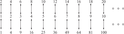
It was the great 16th-century Italian polymath Galileo Galilei (1564–1642) who was first to alert us to the fact that the nature of infinite collections is fundamentally different from finite ones. As alluded to on the first page of this book, the size of a finite set is smaller than that of a second set if the members of the first can be paired off with those of just a portion of the second. However, infinite sets by contrast can be made to correspond in this way to subsets of themselves (where by the term subset I mean a set within the set itself). We need go no further than the sequence of natural counting numbers 1, 2, 3, 4, ··· in order to see this. It is easy to describe any number of subsets of this collection that themselves form an infinite list, and so are in a one-to-one correspondence with the full set (see Figure 8): the odd numbers, 1, 3, 5, 7, ···, the square numbers, 1, 4, 9, 16, ··· and, less obviously, the prime numbers, 2, 3, 5, 7, ···, and in each of these cases the respective complementary sets of the even numbers, the non-squares, and the composite numbers are also infinite.
This rather extraordinary hotel, which is always associated with David Hilbert (1862–1943), the leading German mathematician of his day, serves to bring to life the strange nature of the infinite. Its chief feature is that it has infinitely many rooms, numbered 1, 2, 3, ···, and boasts that there is always room at Hilbert’s Hotel.
8. The evens and the squares paired with the natural numbers
One night, however, it is in fact full, which is to say each and every room is occupied by a guest and much to the dismay of the desk clerk, one more customer fronts up demanding a room. An ugly scene is avoided when the manager intervenes and takes the clerk aside to explain how to deal with the situation: tell the occupant of Room 1 to move to Room 2 says he, that of Room 2 to move into Room 3, and so on. That is to say, we issue a global request that the customer in Room n should shift into Room n + 1, and this will leave Room 1 empty for this gentleman!
And so you see, there is always room at the Hilbert Hotel. But how much room?
The next evening, the clerk is confronted with a similar but more testing situation. This time a spaceship with 1729 passengers arrives, all demanding a room in the already fully occupied hotel. The clerk has, however, learned his lesson from the previous night and sees how to extend the idea to cope with this additional group. He tells the person in Room 1 to go to Room 1730, that of Room 2 to shift to Room 1731, and so on, issuing the global request that the customer in Room n should move into Room number n + 1729. This leaves Rooms 1 through to 1729 free for the new arrivals, and our clerk is rightly proud of himself for dealing with this new version of last night’s problem all by himself.
The final night, however, the clerk again faces the same situation – a full hotel, but this time, to his horror, not just a few extra customers show up but an infinite space coach with infinitely many passengers, one for each of the counting numbers 1, 2, 3. ···. The overwhelmed clerk tells the coach driver that the hotel is full and there is no conceivable way of dealing with them all. He might be able to squeeze in one or two more, any finite number perhaps, but surely not infinitely many more. It is plainly impossible!
An infinite riot might have ensued except again for the timely intervention of the manager who, being well versed in Galileo’s lessons on infinite sets, informs the coach driver that there is no problem at all. There is always room at Hilbert’s Hotel for anyone and everyone. He takes his panicking desk clerk aside for another lesson. All we need do is this, he says. We tell the occupant of Room 1 to shift into Room 2, that in Room 2 to shift to Room 4, that in Room 3 to go to Room 6, and so on. In general the global instruction is that the occupant of Room n should move into Room 2n. This will leave all the odd numbered rooms empty for the passengers of the infinite space coach. No problem at all!
The manager seems to have it all under control. However, even he would be caught out if a spaceship turned up that somehow had the technology to have one passenger for each point in the continuum of the real line. One person for every decimal number would totally overrun Hilbert’s Hotel, and we shall see why in the next section.
All this may be surprising the first time you think about it, but it is not difficult to accept that the behaviour of infinite sets may differ in some respects from finite ones, and this property of having the same size as one of its subsets is therefore a case in point. In the 19th century, however, Georg Cantor (1845–1918) went much further and discovered that not all infinite sets can be regarded as having equally many members. This revelation was unexpected in nature but is not hard to appreciate once your attention is drawn to it.
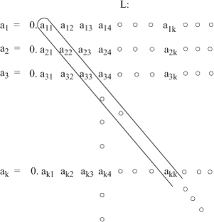
Cantor asks us to think about the following. Suppose we have any infinite list L of numbers a1, a2, ··· thought of as being given in decimal form. Then it is possible to write down another number, a, that does not appear anywhere in the list L: we simply take a to be different from a1 in the first place after the decimal point, different from a2 in the second decimal place, different from a3 in the third decimal place, and so on – in this way, we may build our number a making sure it is not equal to any number in the list. This observation looks innocuous but it has the immediate consequence that it is absolutely impossible for the list L to contain all numbers, because the number a will be missing from L. It follows that the set of all real numbers, that is all decimal expansions, cannot be written in a list, or in other words cannot be put into a one-to-one correspondence with the natural counting numbers, the way we saw in Figure 8. This line of reasoning is known as Cantor’s Diagonal Argument, as the number a that lies outside the set L is constructed by imagining a list of the decimal displays of L as in Figure 9 and defining a in terms of the diagonal of the array.
There is some subtlety here, for we might suggest that we can easily get around this difficulty by simply placing the missing number a at the front of L. This creates an enlarged listing M containing the annoying number a. However, the underlying problem has not gone away. We can apply Cantor’s construction again to introduce a fresh number b that is not present in the new list M. We can of course continue to augment the current list as before any number of times, but Cantor’s point remains valid: although we can keep creating lists that contain additional numbers that were previously overlooked, there can never be one specific list that contains every real number.
9. Cantor’s number a differs from each ak in the kth decimal place
The collection of all real numbers is therefore larger in a sense than the collection of all positive integers. Even though both are infinite, the sets cannot be paired off together the way the even numbers can be paired with the list of all counting numbers. Indeed, if we apply Cantor’s Diagonal Argument to a putative list of all numbers in the interval 0 to 1, the missing number a will also lie in this range. Therefore, we likewise conclude that this collection will also defy every attempt at listing it in full. I mention this as we shall make use of that fact shortly.
Cantor’s result is rendered all the more striking by the fact that many other sets of numbers can be put into an infinite list, including the Greeks’ euclidean numbers. A little ingenuity is involved, but once a couple of tricks are learned, it is not hard to show that many sets of numbers are countable, which is the term we use to mean the set can be listed in the same fashion as the counting numbers. Otherwise an infinite set is called uncountable.
For example, let us take the set of all integers Z, which comes to us naturally as a kind of doubly infinite list. We can, however, rearrange it into a row with a starting point: 0, 1, −1, 2, −2, 3, −3, ··· by pairing each positive integer with its opposite, we create a list where every integer appears – none will escape. More surprisingly, we can also do the same with the rationals: start with 0, then list all the rationals that can be written using all numbers no more than 1 (which are 1 and −1), then those that involve no number higher than 2 (which are 2, −2,  ), then those that only use numbers up to 3, and so on. In this way, the fractions (positive, negative, and zero) can be arranged in a sequence in which they are all present and accounted for. The rationals therefore also form a countable set, as do the euclidean numbers, and indeed if we consider the set of all numbers that arise from the rationals through taking roots of any order, the collection produced is still countable. We can even go beyond this: the collection of all algebraic numbers (first mentioned in Chapter 6), which are those that are solutions of ordinary polynomial equations, form a collection that can, in principle, be arrayed in an infinite list: that is to say, it is possible to describe a systematic listing that sweeps them all out. (The proof is along the lines of the argument that works for the rationals.)
What we have allowed to happen in casually accepting any decimal expansion is to open the door to what are known as the transcendental numbers, those numbers that lie beyond those that arise through euclidean geometry and ordinary algebraic equations. Cantor’s argument shows us that transcendental numbers exist and, in addition, there must be infinitely many of them, for if they formed only a finite collection, they could be placed in front of our list of algebraic numbers (the non-transcendentals), so yielding a listing of all real numbers, which we now know is impossible. What is striking is that we have discovered the existence of these strange numbers without identifying a single one of them! Their existence was revealed simply through comparing certain infinite collections to one another. The transcendentals are the numbers that fill the huge void between the more familiar algebraic numbers and the collection of all decimal expansions: to borrow an astronomical metaphor, the transcendentals are the dark matter of the number world.
In passing from the rationals to the reals, we are moving from one set to another of higher cardinality as mathematicians put it. Two sets have the same cardinality if their members can be paired off, one against the other. What can be shown using the Cantor argument is that any set has a smaller cardinality than the set formed by taking all of its subsets. This is obvious for finite collections: indeed, in Chapter 5 it was explained that if we have a set of n members then there are 2n subsets that can be formed in this way. But how large is the set S of all subsets of the infinite set of natural numbers, {1, 2, 3, ···}? This question is not only interesting in itself but also in the manner in which we arrive at the answer, which is that S is indeed uncountable.
Suppose to the contrary that S was itself countable, in which case the subsets of the counting numbers could be listed in some order A1, A2, ···. Now an arbitrary number n may or may not be a member of An – let us consider the set A that consists of all numbers n such that n is not a member of the set An. Now A is a subset of the counting numbers (possibly the empty subset) and so appears in the aforesaid list at some point, let A = Aj say. An unanswerable question now arises: is j a member of Aj? If the answer were ‘yes’ then, by the very way A is defined, we conclude that j is not a member of A, but A = Aj, so that is self-contradictory. The alternative is no, j is not a member of Aj, in which case, again by the definition of A, we infer that j is a member of A = Aj, and once more we have contradiction. Since contradiction is unavoidable, our original assumption that the subsets of the counting numbers could be listed in a countable fashion must be false. Indeed, this argument works to show that the set of all subsets of any countable but infinite set is uncountable.
This particular self-referential style argument was introduced by Bertrand Russell (1872–1970) in a slightly different context that led to what is known as Russell’s Paradox. Russell applied it to the ‘set of all sets that are not members of themselves’, asking the embarrassing question whether or not that set is a member of itself. Again, ‘yes’ implies ‘no’ and ‘no’ implies ‘yes’, forcing Russell to conclude that this set cannot exist.
In the 1890s, Cantor himself discovered an implicit contradiction stemming from the idea of the ‘set of all sets’. Indeed, Russell acknowledged that the argument of his paradox was inspired by the work of Cantor. The upshot of all this, however, is that we cannot simply imagine that mathematical sets can be introduced in any manner whatsoever, but some restrictions must be placed on how sets may be specified. Set theorists and logicians have been wrestling with the consequences of this ever since. The most satisfactory resolution of these difficulties is provided by the now standard ZFC Set Theory (the Zermelo-Fraenkel set theory with the Axiom of Choice).
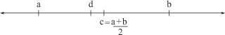
There are different ways of looking at the size of infinite sets of numbers that are revealed if we look at the distribution of the various number types that knit together to bind the number line into a continuum. The rationals may only be a countable collection of numbers, but the collection is densely packed within the line in a way that the integers plainly are not. Given any distinct numbers, a and b, there is a rational number that lies between them. The average of the two numbers, c =  , certainly is a number lying between them, but it may be irrational. However, if c is irrational we can approximate it by a rational number d, with a terminating decimal expansion, by letting d have the same decimal representation as c up to a very large number of decimal places. For example, if we take
  = 1.414···, we have that differs from 1.414 by less than 0.001, and each time we take another decimal place we guarantee finding a rational number that approximates more accurately (on average, ten times more accurately) than the previous one. If the number of initial places in which they agree is sufficiently large, then their difference will be so small that both c and d will lie between a and b. The number of places we need to take after the decimal place will depend on just how close a and b are to each other to begin with, but it is always possible to find a rational d that does the job (see Figure 10). We say that the set of rational numbers is dense in the number line for just this reason. Of course we can, by the same argument, show that there is another rational, splitting the interval from a to d, say, and, in this way, we arrive at the conclusion that infinitely many rational numbers lie between any two numbers, however small the difference between these two numbers might happen to be. In particular, there is no such thing as the smallest positive fraction, for, given any positive number, there is always a rational lying between it and zero.
Not to be outdone, the set of irrationals also forms a dense set. Before explaining this, I point out that once we have identified one irrational, the Pythagorean number for example, the floodgates open and we can immediately identify infinitely more. When we add a rational to an irrational the result is always an irrational. For example, + 7 is irrational by dint of this fact. In a similar fashion, if we multiply an irrational number by a rational number (other than 0), the result is another irrational number. (Simple contradiction arguments establish both these claims.) In particular, we can find an irrational number of size as small as we like:  is irrational for any counting number n and by taking n larger and larger we can make t as close to 0 as we please. As with the rationals, we therefore see that there is no smallest positive irrational, and hence there is no such thing as the smallest positive number.
10. Rationals separate any given positions on the number line
Returning to our given numbers, a and b, once again let c be their average. If c is irrational, we have a number of the required kind (irrational). If on the other hand, c is rational, put d = c + t, where t is the irrational number of the previous paragraph. By what has gone before, d will also be irrational, and if we take n large enough, we can always ensure that d is so close to the average c of the two given numbers a and b that it lies between them. In this way, we see that the irrational numbers too form a dense set and, as with the rational numbers, we can infer that there are infinitely many irrational numbers lying between any two numbers on the number line.
And so the set of rationals and its complementary set of irrationals are in one way comparable (they are both dense in the number line) and in another not (the first set is countable, the second not).
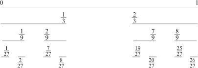
We now have a clearer idea as to how the rational and the irrational numbers interlace to form the real number line. The rational numbers form a countable set, yet are densely packed into the number line. Cantor’s Middle Third Set is, by way of contrast, an uncountable subset of the unit interval that nevertheless is sparsely spread. It is the result of the following construction.
We begin with the unit interval I, that is all the real numbers from 0 up to 1 inclusive. The first step in the formation of Cantor’s set is the removal of the middle third of this interval, that is all the numbers between  and
and  . The set that remains consists of the two intervals from 0 up to and from
  up to 1. At the second stage, we remove the middle third of these two intervals, at the third stage we remove the middle third of the remaining intervals, and so on. Cantor’s Middle Third Set C then consists of all points of I that are not removed at any stage of this process.
11. Evolution of Cantor’s Middle Third Set to the 4th level
The total length of the little intervals that remain as we pass from one stage of this process to the next is, by design, that of the previous stage; it follows that at the nth stage the total length of the surviving intervals is ()n. This expression approaches 0 as n increases and since the Cantor set C is the collection of all points that are left at the end of it all, it follows that the ‘length’, or measure, of C must be 0.
We might suspect that we have thrown the baby out with the bath water and that there are no points at all left in C. Is the Middle Third Set empty? The answer is a resounding no! There are infinitely many numbers left in C. This is best seen if we shift our representation of the numbers of the interval to base three ‘decimals’ known as ternary, as the whole construction is based on thirds. In base three decimals, the numbers and are respectively given by 0.1 and 0.2. By discarding the middle third of the unit interval, we have thrown away all those numbers whose ternary expansion begins with 0.1, and indeed the overall process weeds out exactly those numbers that have a 1 anywhere in their ternary expansions. The numbers in C are exactly those whose ternary expansions consist entirely of 0s and 2s. (For example,  survives the infinite cull as in ternary it has the recurring expansion 0.202020 ‥ ‥)
Next we make an amazing observation. By taking the ternary expansion of any number c in C and replacing each instance of 2 by 1, we obtain the binary expansion of some number c in the unit interval. This gives a one-to-one correspondence of C with the set of all numbers in I (written in binary). It follows that the cardinality of C is the same as that of I, and since the latter is an uncountable set (by Cantor’s Diagonal Argument), it follows that the Cantor Middle Third Set is not only infinite but uncountable.
Therefore we have a set C that is in one sense negligible in size (has measure zero), but by another way of reckoning C is huge, as it has the same cardinality as I and hence of the whole real line.
What is more, far from being dense, C is nowhere dense. Recall that by saying that a set like the rationals is dense, we mean that whenever we take a real number a, there are rational numbers to be found in any little interval surrounding a, however small that interval might be. We say that any neighbourhood of a contains members of the set of rationals. The Cantor set has quite the opposite nature – numbers not in C might live their lives in the real line without ever coming across any members of C, provided they confine their experiences to a narrow enough locality around where they live. To see this, take any number a that is not in C, so that a has a ternary expansion that contains at least one 1: a = 0 · … .1 … ‥, with the 1 in the nth place, say. For a sufficiently tiny interval surrounding a, the numbers b in that interval have a ternary expansion that agrees with that of a up to places beyond the n th, and so all of them will also not be members of the strange set C as their ternary expansions will also contain at least one instance of 1.
On the other hand, any member a of the Cantor set will not feel too isolated, for when a looks out into any interval J that surrounds it in the number line, however small, a will find neighbours from the set C living alongside it (and numbers not in C as well). We can specify a member b of the given interval J that also lies in C by taking b to have a ternary expansion that agrees with a to a sufficiently large number of places, but with no entry being a 1. Indeed, there are uncountably many members of C in J.
In conclusion, the Cantor Middle Third Set C is as numerous as can be and, to the members of the C club, their brothers and sisters are to be seen all around them wherever they look. To the numbers not in C, however, C hardly seems to exist at all. Not one member of C is to be spotted in their exclusive neighbourhoods, and the set C itself has measure zero. To them, C is almost nothing.
Some of the principal sets of the number line may be characterized in the language of equations. The rational numbers, which form a countable set, are the numbers that arise as solutions of simple linear equations: the fraction  is the solution to the equation ax − b = 0 (a and b are integers). Numbers like that do not arise in this way are called irrational, and they form an uncountable collection that cannot be paired off with the counting numbers in the way that the rationals can. Within the set of irrationals there are the transcendentals, which are the numbers that never arise as the solutions of equations of these kinds even if we allow higher powers of x. It is known that π is an example of a transcendental number, but is not, as it solves the equation x2 − 2 = 0. The approach then is to define classes of numbers through the kinds of equations they solve.
An interesting line of study emerges, however, when we take the opposite tack and insist that not only the coefficients of our equations but their solutions have also to be integers. Here is a classic example.
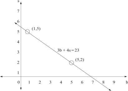
A box contains spiders and beetles and 46 legs. How many of each kind of creature are there? This little number puzzle can be solved easily by trial, but it is instructive to note that first, it can be represented by an equation: 6b + 8s = 46, and second that we are only interested in certain kinds of solutions to that equation, namely those where the number of beetles (b) and spiders (s)are counting numbers. In general, a system of equations is called Diophantine when we are restricting our solution search to special number types, typically integer or rational answers are what we are after.
There is a simple method for solving linear Diophantine equations such as this one. First, divide through the equation by the hcf of the coefficients, which are in this case 6 and 8 so their hcf is 2. Cancelling this common factor of 2 we obtain an equivalent equation, that is to say one with the same solutions: 3b + 4s = 23. If the right-hand side were no longer an integer after performing this division, that would tell us that there were no integral solutions to the equation and we could stop right there. The next stage is to take one of the coefficients, the smaller one is normally the easiest, and work in multiples of that, in this case 3. Our equation can be written as 3b + 3s + s = (3 × 7) + 2; rearranging we obtain s = (3 × 7) − 3b − 3s + 2. The point of this is that it shows that s has the form 3t + 2 for some integer t. Substituting s = 3t + 2 into our equation and making b the subject, we get
3b + 4(3t + 2) = 23 ⇒ 3b = 15 − 12t ⇒ b = 5 − 4t.
We now have the complete solution in integers to the Diophantine equation: b = 5 − 4t, s = 3t + 2. Choosing any integral value for t will give a solution, and all solutions in integers are of this form.
Our original problem, however, was further constrained in that both b and s had to be at least zero, as negative beetles and spiders do not exist. Hence there are only two feasible values of t, those being t = 0 and t = 1, giving us the two possible solutions of 5 beetles and 2 spiders, and 1 beetle and 5 spiders. If we interpret the puzzle as meaning that there is a plurality of both types of creature, we have the traditional solution: 5 beetles and 2 spiders.
12. Lattice points on the line of a linear equation
This type of problem is called linear because the graph of the associated equation consists of an infinite line of points. The Diophantine problem then is to find the lattice points on this line, which are the points where both coordinates are integral or, if we only admit positive solutions, only lattice points in the positive quadrant will do.
However, once we allow squares and higher powers into our equations, the nature of the corresponding problems are much more varied and interesting. A classical problem of this type that has a full solution is that of finding all Pythagorean triples: positive integers a, b, and c such that a2 + b2 = c2. A Pythagorean triple of course takes its name from the fact that it allows you to draw a right-angled triangle with sides of those integer lengths. The classic example is the (3, 4, 5) triangle. Given any Pythagorean triple, we can generate more of them simply by multiplying all the numbers in the triple by any positive number as the Pythagorean equation will continue to hold. For example, we can double the previous example to get the (6, 8, 10) triple. This, however, gives a similar triangle, one of exactly the same proportions, as the change is only a matter of scale and not of shape. Given the first triangle, we find the second Pythagorean triple simply by measuring the lengths of the sides in units that are half the size of the original units, thereby doubling the numerical size of the dimensions. There are, however, genuinely different triples such as those representing the (5, 12, 13) and the (65, 72, 97) right-angled triangles.
In order to describe all Pythagorean triples, therefore, it is enough to do the job for all triples (a, b, c) where the hcf of the three numbers is 1, as all others are merely scaled-up versions of these. The recipe is as follows. Take any pair of coprime positive integers m and n, with one of them even, and let m denote the larger. Form the triple given by a = 2mn, b = m2 − n2 and c = m2 + n2. The three numbers a, b, and c then give you a Pythagorean triple (the algebra is easily checked) and the three numbers have no common factor (also not difficult to verify). The three examples above arise by taking m = 2 and n = 1 in the first case, m = 3 and n = 2 in the second, while for the last triangle we have m = 9, n = 4. It takes more work to verify the converse: any such Pythagorean triple arises in this fashion for suitably chosen values of m and n, and what is more, the representation is unique so that two different pairs (m, n) cannot yield the same triple (a, b, c).
The corresponding equation for cubes and higher powers has no solution at all: for any power n ≥ 3, there are no positive integer triples x, y, and z such that xn + yn = zn. This is the famous Fermat’s Last Theorem, which in future might be known as Wiles’s Theorem as it was finally proved in the 1990s by Sir Andrew Wiles. Even for the case of cubes, first solved by Euler, this is a very difficult problem. It is, however, relatively easy to show that the sum of two fourth powers is never a square (and so certainly not a fourth power). This is enough to reduce the problem to the case where n is a prime p (meaning that if we solved the problem for all prime exponents, the general result would follow at once), and indeed the problem was solved for so-called regular primes in the 19th century. However, the full solution was only realized as a consequence of Wiles settling a deep question called the Shimura–Taniyama Conjecture.
The most intensively investigated Diophantine equation is, however, the Pell equation, x2 − ny2 = 1, where n is a positive integer that is not itself a square. Its significance was appreciated very early, for it seems it was studied both in Greece and in India perhaps as far back as 400 BC, because its solution allows good rational approximations,  of
of  . For example, when n = 2, the equation has as one solution pair the numbers x = 577 and y = 408, and ()2 = 2.000006. The equation is related to the geometric process of what the Greeks called anthyphairesis where one begins with two line segments and continues to subtract the shorter from the longer, a kind of analogue of the Euclidean Algorithm but applied to continuous lengths. Indeed, the Archimedes Cattle Problem mentioned in Chapter 5 leads to an instance of the Pell equation.
Versions of the Pell equation were studied by Diophantus himself around AD 150 but the equation was solved by the great Indian mathematician Brahmagupta (AD 628) and his methods were improved upon by Bhaskara II (AD 1150), who showed how to create new solutions from a seed solution. In Europe, it was Fermat who exhorted mathematicians to turn their attention to Pell’s equation and the complete theory is credited to the reknowned French mathematician Joseph-Louis Lagrange (1736–1813) (the English appellation ‘Pell’ is an historic accident). The general method of solution is based on the continued fraction expansion of .
Recall the sequence of numbers, 1, 1, 2, 3, 5, 8, 13, 21, ··· discovered by Fibonacci and introduced in Chapter 5. Take a pair of successive terms in this sequence and write the corresponding ratio as 1 plus a fraction. If we now ‘Egyptianize’ this fraction by repeatedly dividing top and bottom by the numerator, a striking pattern emerges. Take, for instance
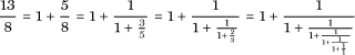
We obtain a multi-floored fraction consisting entirely of 1s, and each preceding ratio of Fibonacci numbers appears as we wind through the calculation. This must happen every time: by the very way these numbers are defined, each Fibonacci number is less than twice the next, and so the result of the division will leave a quotient of 1 and the remainder is the preceding Fibonacci number. You will recall that the ratio of successive Fibonacci numbers approaches the Golden Ratio, τ, and so this suggests that τ is the limiting value of the continued fraction consisting entirely of 1s.
As was shown in Chapter 5, the value of an infinite repeating process may be made the subject of an equation based on that process. If we call the value of the infinite fractional tower of 1s by the name a, we see that a satisfies the relation a = 1 +  because what lies underneath the first floor of the fraction is just another copy of a. From this, we see that a satisfies the quadratic equation a2 = a + 1, the positive root of which is τ =
The type of continued fractions that emerge from this process are intrinsically important. When we approximate an irrational number y by rationals we naturally turn to the decimal representation of y. This is excellent for general calculations but, being tied to a particular base, is not mathematically natural. Essential to the nature of y is how well our number y can be approximated by fractions with relatively small denominators. Is there any way to find a series of fractions that best deals with the conflicting demands of approximating y to a high degree of accuracy while keeping the denominators relatively small? The answer lies in the continued fraction representation of a number that does this through its truncations at ever lower floors.
Continued fractions look very awkward because of the many floors we have used in representing them. However, the inconvenience of writing all the floors of the division is easily side-stepped – since every numerator is 1, we need only record the quotients in the division to specify which continued fraction we are talking about. For instance, the representation for the fraction  develops as follows:
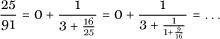
that eventually yields a continued fraction specified by the list [0, 3, 1, 1, 1, 3, 2]. As we have seen, the Golden Ratio, τ has the continued fraction representation [1, 1, 1, 1, ···]. In a fashion reminiscent of repeating decimal notation, we write τ = [Ī]. The first instance of 3 in the continued fraction of comes from writing 91 = 3 × 25 + 16, which is the first line in the Euclidean Algorithm for the pair (91, 25). Indeed, for this very reason there is one line in the continued fraction for every line of the algorithm when performed on the two numbers. In particular, starting with a reduced fraction in which the two numbers are coprime, the same will apply to each of the fractions that arise in the course of the calculation of the corresponding continued fraction.
The special example afforded by the Golden Ratio opens the door to the idea that we may be able to represent other irrational numbers not by finite continued fractions (which are obviously just rational themselves) but by infinite ones. But how is the continued fraction of a number a produced? The reader will need to tolerate a little algebraic trickery in order to see this in action, but here is how it goes.
There are two steps in the calculation of a continued fraction for a number a = [a0, a1, a2,···]. The number a0 is the integer part of a, denoted by a0 = a.(For example, the integer part of π = 3.1415927 ··· is given by [π] = 3.) In general, an = rn, the integer part of rn, where the remainder term rn is defined recursively by r0 = a, rn =  Applying this for example to a = and employing the algebraic device of rationalizing the denominator (with which some readers may be familiar) we obtain, since [] = 1:
a = r0 = = 1 + ( − 1) so that a0 = 1;

Next we get

so that r1 = r2 = ···= + 1, a1 = a2 = ···= 2, and so = [1, 2].
Indeed, the numbers that have recurring representations as continued fractions are rational numbers (which are exactly the ones whose representations terminate) and those that arise from quadratic equations such as τ, which we saw above is one solution of the equation x2 = x + 1, and =  which satisfies x2 = 2. Some other examples showing the rather unpredictable nature of the recurrences are
  =
= 
 =
= 
 =
=  and 8 =
  There is nevertheless one very particular and remarkable facet to the pattern of the expansion of the continued fraction of an irrational square root. The expansion begins with an integer r, and the recurrent block consists of a palindromic sequence (a sequence of numbers that reads the same in reverse) followed by 2r. This can be seen in all the preceding examples: for instance for 8 we see that r = 5, the palindromic part of the expansion is 3, 2, 3, which is followed by 2r = 10. For and , the palindromic part is empty, but the pattern is still there, albeit in a simple form. It can be shown that the continued fraction representation of a number is unique – two different continued fractions have different values.
The importance of continued fractions in approximation of irrationals by rationals is due to the so called convergents of the fraction, which are the rational approximations of the original number that result from truncating the representation at some point and working out the corresponding rational number. These represent the best approximation possible to the number in question in the sense that any better approximation will have a larger denominator than that of the convergents. The convergents of the Golden Ratio are the Fibonacci ratios. Since every term in the continued fraction representation of τ is 1, the convergence of these ratios is retarded as much as it possibly could be. For that reason, there is no more difficult number than τ to approximate by rationals and the Fibonacci ratios are the best you can do.
If the denominator of a convergent of a continued fraction is q, then the approximation is always within  of the true value of the number and the convergents of a continued fraction alternately underestimate and overestimate the value to which they approach. It is, however, the euclidean numbers such as τ and that are the worst when it comes to rational approximation. Some particular transcendentals, whose nature may seem the farthest removed from the rational world, may yet be approximated very closely and have convergents that home in on the target number with great rapidity.
The connection with Pell’s equation, x2 − ny2 = 1, mentioned at the close of the previous section, now comes about as the solution (x, y) to the equation with the minimum possible positive value of x exists and is to be found among the convergents of the continued fraction representation of . For example, when n = 7 the sequence of convergents of begins with 2/1, 3/1, 5/2, 8/3, ··· and it is x = 8, y = 3 that provides this smallest so called fundamental solution of the Pell equation x2 − 7y2 = 1. The fundamental solution, however, sometimes does not turn up at all early in the expansion: for example, the smallest positive solution to x2 − 29y2 = 1is x = 9801 and y = 1820. Once this fundamental solution (x, y) has been located, however, all other solutions arise by taking successive powers of the expression (x + y)k (k = 1, 2, 3, ···) and extracting the coefficients of the corresponding rational and irrational parts of the expanded expression. In this way, the full solution set of the Pell equation is realized through the continued fraction representation of .