In this chapter, we will be looking at thermodynamics — the kinetic theory of heat — from both macroscopic and microscopic perspectives. The zeroth and first law of thermodynamics will be introduced and applied to the specific system of an ideal gas.
It is common knowledge that if we put a hot object in thermal contact with a cool object, the hot object becomes cooler while the cool object becomes hotter to a certain extent. This is a quotidian phenomenon that occurs until the transfer of “hotness” or “coolness” between the two objects ceases. At this juncture, the two objects have attained thermal equilibrium. Specifically, two objects are said to be in thermal equilibrium if they are in thermal contact and there is no net exchange of heat between them. We will hold off the definition of heat for now and just understand it as a form of energy transfer. Finally, when thermal equilibrium is attained between two objects, they should be similar in a certain respect — if two systems are in thermal equilibrium, they are said to possess the same temperature.
The zeroth law of thermodynamics states that if objects A and B are each at thermal equilibrium with a common object C, objects A and B are at thermal equilibrium with each other. This intuitive concept has vast consequences. Firstly, it standardizes the notion of temperature as the definition of temperature now implies that all objects of the same temperature are in thermal equilibrium. Next, the zeroth law allows us to use object C to determine whether objects A and B will be in thermal equilibrium without physically putting them in thermal contact. This, combined with the fact that object C may experience certain measurable and observable changes when placed in contact with objects A and B, such as a rise in the mercury level due to expansion in a mercury thermometer or the change in the pressure of a gas, allows us to quantify the temperature of an object. For example, we can have two reference points, setting 0°C for ice and 100°C for steam, and divide the interval into 100 equal segments to create the Celsius temperature scale.
In thermodynamics, it is important to distinguish between state variables and non-state variables. As its nomenclature implies, state variables — such as pressure, volume and temperature — are functions of the configuration of a system which can be specified by the positions and velocities of all constituents in a system.
Non-state variables are not functions of the configuration of the system and can thus have multiple values at a single state. Consider a car driving from the origin in the xy-plane, stocked with a certain initial amount of fuel. If we define the state of the car to be its position in the xy-plane, the amount of fuel left in the car at a given state is not a state function as the car can traverse different paths to reach the same final state — these paths may consume different amounts of fuel. Most starkly, if the car drives back to the origin, the amount of fuel left is not the same as before! Therefore, the amount of fuel left in the car is definitely not a state variable as we cannot determine its value solely by looking at the car’s position.
The internal energy of a system is defined to be the sum of all microscopic forms of energy — energy on the atomic and molecular scale. It is the sum of all microscopic kinetic energy and microscopic potential energy. Crucially, internal energy is uniquely defined for each state of a system and is a state variable.
Microscopic kinetic energy results from the possible random motions of individual constituents. For example, molecules may translate, rotate and even vibrate about a common center. The latter two situations only occur in the case of polyatomic molecules. It is important to differentiate microscopic and macroscopic kinetic energies. The former is highly disordered and thus less useful than the latter, to a certain extent. A moving block has a macroscopic kinetic energy associated with the motion of the entire object as a whole but if we zoom into the scale of individual molecules, we may find them jiggling about in random directions and thus can associate a microscopic kinetic energy with that motion.
Microscopic potential energy results from the interactions between the constituents of a system and between the constituents of a system and external factors, on a molecular scale. Chemical bonds between atoms and strong interactions in the nuclei are typical examples of internal interactions. The creation of electric dipoles in atoms due to an external electric field is an example of an interaction with an external entity. A special form of internal interactions, associated with the phase of a system, results in a form of energy known as latent energy. This will be explored in a later chapter.
Heat and work are both energies in transit and are not forms of energy. In the case of closed systems where mass exchange cannot occur, heat and work are the only possible forms of energy transfer. Similar to how the work performed on a particle increases its macroscopic kinetic energy in mechanics, heat and work are just methods of delivering or extracting energy. However, heat can be differentiated from work by observing that its flow requires a temperature gradient. Work, on the other hand, can be performed by a system on another system of the same temperature. For example, two gases, that are separated by a movable wall, may have attained the same temperature but not the same pressure. Then, there is work performed by pushing the wall.
Heat and work done are not state variables as they are just methods of delivering energy to or extracting energy from a system. For the same change in the internal energy of a system which is a state variable, heat and work done can make different contributions to this change, as long as their sum is consistent. Moreover, their final products — namely the change in internal energy of the relevant system — are indistinguishable, so there is no way to deduce their individual contributions by observing the final state of the system alone. This is analogous to how it is impossible to know what your sneaky friend has spent your credit card on by simply analyzing the total amount of money left in your bank account — you have to inspect the bill at the end of the month which details every single purchase (the process of purchasing). Therefore, heat and work done are, most importantly, both process-dependent.
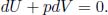
The first law of thermodynamics is quintessentially the conservation of energy. Supposing that there is a decrease in the internal energy and macroscopic kinetic energy of a system, this decrease in energy should manifest itself as the physical work done by the system and the heat flowing from the system. Conversely, we can conclude that the increase in the internal energy plus macroscopic kinetic energy of a system is the sum of the heat supplied to and the work done on the system. This is the first law of thermodynamics which can be expressed mathematically as

where Won is the net work done on the system by external agents and Q is the net heat supplied to the system. The conservative work on the right-hand side can be shifted to the left-hand side such that the left-hand side becomes the change in the system’s total energy E (internal energy plus macroscopic kinetic and potential energies).

where Won now only includes the work done by non-conservative forces on the system. Usually, the macroscopic energies are constant such that the above becomes

In most cases, the heat transferred between systems is prohibitively difficult to determine directly. However, the first law enables us to calculate heat indirectly from measurable quantities such as internal energy and work done.
Sometimes, the first law is expressed in terms of the work done by the system, which is negative of the work done on the system, Wby = –Won. Then,

In a certain sense, the heat supplied to the system manifests in terms of the work performed by the system and the increase in internal energy as it stores part of the heat.
Now, we are interested in analyzing the specific system of gases. Microscopically, we can model a gas as a system of molecules that are hard spheres undergoing constant random motion. These particles are assumed to collide elastically, have no interactions with one another (besides collisions) and are small relative to the volume of their container. A gas that exhibits such behavior is known as an ideal gas and is of course, not realistic. When gas particles collide with the walls of the container, they exert a force on the walls of the container. Macroscopically, these collisions manifest as a pressure on the container walls.
A system is in thermodynamic equilibrium when the macroscopic state of every part of the system is not evolving over time. A pressure and temperature can be defined for every part of a gas at equilibrium. However, if the gas were to undergo a sudden change, such as a contraction, it will be in a non-equilibrium state, at least for a short instance. Then, a pressure and temperature are not well-defined at this juncture.
We can define the equilibrium state of an ideal gas using three state variables — temperature, pressure and volume. For a system in general, there will be an equation that relates the different state variables. In the particular case of an ideal gas, its equation of state is known as the ideal gas law. Concretely,

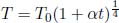
where p, V and T are the pressure, volume and the temperature of the gas respectively. n is the number of moles of gaseous molecules while R is the ideal gas constant, R = 8.314 J mol–1K–1. Note that T is measured in Kelvins, which can easily be calculated from a temperature expressed in degree Celsius with the following conversion formula:

The ideal gas law makes intuitive sense from a microscopic standpoint, it basically states that

When the number of moles of molecules increases, more molecules collide with the walls per unit time — increasing the pressure of the gas. When temperature increases, the gaseous molecules become more “excited” and possess a larger average kinetic energy. Thus, they exert a greater force on the container walls per collision and collide with the walls more frequently. Lastly, if the volume of the container is increased, gaseous molecules have to travel a longer distance to collide with the walls, leading to a decrease in the frequency of collision and hence pressure. Another slight technicality is that n strictly refers to the number of moles of gaseous molecules and not the total moles of gaseous particles or atoms. Even if the container encloses k moles of diatomic gaseous molecules, n is still equal to k and not 2k. The number of elementary entities in a mole is the Avogadro’s Constant, NA = 6.02 × 10²³. Thus, we can rewrite the ideal gas equation in terms of the number of gaseous molecules.

where N is the total number of molecules and k =  = 1.38 × 10⁻²³JK–1 is the Boltzmann constant.
Ultimately, the ideal gas law encapsulates the following three gas laws which are its predecessors. Firstly, Boyle’s law states that the pressure and volume of a gas of fixed mass are inversely proportional when its temperature is held constant. Secondly, Charles’ law states that the absolute temperature (Kelvin scale) and volume of a gas of fixed mass are directly proportional when its pressure is held constant. Finally, Gay–Lussac’s law asserts that the pressure and absolute temperature of a gas of fixed mass are directly proportional when its volume is held constant.
Problem: A thermally insulated piston of negligible dimensions separates a rectangular container into two regions. The two regions are both filled with ideal gases at an initial temperature of 27°C. The initial configuration of the system is shown in Fig. 2.1, with the piston being initially stationary. The temperature of the gas in region A is now increased to 227°C while the temperature of the gas in the other region is maintained at 27°C. Find x, the distance of the piston from the left end of the container, after the system has equilibrated.
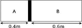
Figure 2.1:Ideal gases
Let the cross sectional area of the container be A. For the system to be at equilibrium, the pressures due to both gases should be equal. Let the initial and final common pressures be p1 and p2 respectively. Since the number of moles of each gas is constant, by the ideal gas equation,

Applying this relation to gases A and B,

Solving,

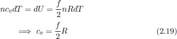
Due to the proposed lack of interactions between ideal gas molecules, the internal energy of an ideal gas stems solely from the microscopic kinetic energy of the moving molecules. By the equipartition theorem in statistical mechanics, energy is shared equally at thermal equilibrium among the modes1 of a molecule — which arise for each independent contribution to the total energy that is quadratic in a certain variable — such as translational and rotational kinetic energy. Each mode of a molecule contributes an additional  kT amount of average energy to a molecule. Due to the lack of internal interactions between molecules, the average energy of a molecule must also be the average kinetic energy. Consequently, the average kinetic energy of a gas molecule is

where f is the number of degrees of freedom of a particle which is the number of independent forms of motion exhibited by a molecule and is also the number of coordinates required to specify the state of a molecule. Then, the internal energy of an ideal gas is

As expected, the internal energy is a state function as it is only dependent on the temperature of the gas. Ideal gases are usually assumed to be monoatomic. Thus, molecules have three degrees of freedom due to possible translations in the x, y and z-directions. This monoatomic property is usually assumed by default unless stated otherwise. For a diatomic gas molecule, there are usually 5 degrees of freedom due to there being three translational and two rotational directions. There are only two rotational degrees of freedom for a diatomic molecule as it is not possible for the diatomic molecule to rotate about the axis joining the two atoms as the atoms are assumed to be small (thus contributing negligible energy due to rotations along this axis). In the general case of polyatomic molecules, vibrational modes may arise, especially at high temperatures. However, we will only be dealing with molecules with no vibrational freedom.
Following from the above discussion, the average translational kinetic energy per molecule of an ideal gas (regardless of the number of atoms per molecule) is
Then, we can actually relate temperature to the mean square speed2 of the molecules. Assuming that there are N gaseous molecules which each have mass m,

The mean square speed  and the root-mean-square speed of the molecules vrms are defined as

We can rewrite the expression for the average kinetic energy per molecule as

to conclude that
This implies that temperature can be used as a direct measure of how fast gas molecules are moving and gives a kinetic interpretation of temperature. Lastly, note that the above expressions for the mean square speed and the root-mean-square speed are consistent with the kinetic theory of gases (as we shall show) — a microscopic model of ideal gases that will be introduced later.
Recall that the infinitesimal work done by a force F in moving an object (such as a wall) is

where dr is the infinitesimal displacement of the object. The differential in front of W is a small δ which represents an inexact differential, as W is not an actual function and thus does not have a derivative. This is because W is generally not a state function and is dependent on the path that a process takes. Moreover, remember that in the case of a fluid, the force that it exerts can only be perpendicular to its surface as it cannot withstand any shear forces. Then, the work done by an infinitesimal portion of gas near the boundary of our gaseous system on its surroundings across a massless interface of surface area dA can be rewritten as pexdAdx, where dx is the signed displacement of the massless interface in the direction of its area vector (defined to be positive outwards with respect to the gas) such that dAdx is the area swept by the infinitesimal interface. Integrating over the entire boundary surface of the gas, the total work done by the gas on its surroundings after an infinitesimal change is

where dV is the change in volume of the gas. It is pivotal to understand that pex refers to the external pressure imposed on the interface by the surroundings and is not the pressure of our gaseous system. It is assumed that the external pressure is well-defined, such as in the case of a force evenly distributed on a massless piston, else the above expression cannot be used either. This dependence on the external pressure can be easily verified in the case where pex = 0 such that even if the gas had a well-defined pressure, it should not perform any work on its surroundings as it will just expand freely. The deeper reason behind is that generally, when the gas pressure initially differs from pex, the gas pressure will be ill-defined at the next instance as the gas will become inhomogeneous. Since the gas sections immediately adjacent to the interface must balance the force enforced by the external pressure, their volumes are changed slightly such that their pressure (assuming that we consider small enough sections which are approximately homogeneous) are accustomed to the external pressure. However, this information is not instantaneously transmitted to other parts of the gas such that the gas is no longer in equilibrium as a whole. All-in-all, the work done by the gas on its surroundings is that due to the sections surrounding the interface which have pressure pex.
Observe that δWby is generally an unedifying description of the evolution of our gaseous system as we are unable to relate it to the gas pressure. However, in the case where the initial gas pressure differs from the external pressure by an infinitesimal value, the infinitesimal work done can be written as

where p is the pressure of the gas, that is also the external pressure. In order for Eq. (2.11) to be valid, the external pressure can only be varied by infinitesimal amounts (e.g. by carefully placing grains of sand on a piston), such that the system evolves over a series of purely equilibrium states from an initial to final state. Such a slowly-occuring process is known as a quasistatic process and is an idealization. Actually, the condition for the applicability of Eq. (2.11) is much stricter — it requires the process that the gas undergoes to be reversible,3 under which being quasistatic is a mere prerequisite. For example, when a gas in a container is undergoing quasistatic compression performed by adding grains of sand on top of a gas piston, the gas pressure will generally differ from the external pressure if friction between the piston and the container walls is present. This friction is in fact a form of irreversiblity which renders Eq. (2.11) obsolete. Therefore, we must scrutinize the circumstances in the problems we face to check if we can apply Eq. (2.11) which is only valid for reversible processes.
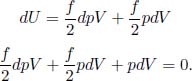
The total work done during a reversible process is obtained by integrating the infinitesimal work done over the path that a system takes.

where the integral indicates that we should track all infinitesimal volume changes as the gas evolves from an initial to final state. When a gas expands, the work done by the gas is positive as the displacement of the interface is in the same direction as the force due to gaseous pressure while the work done on the gas is negative. In a similar vein, when a gas contracts, the work done by the gas is negative and the work done on the gas is positive.
Problem: n moles of helium are isolated in a gas piston with initial temperature T0. If a constant force F is abruptly exerted on the piston for a short period of time such that it contracts the gas by a distance x, determine the final temperature of the gas T1.
In this scenario, the gas does not undergo a reversible process as the change is sudden — implying that we must use the external pressure  where A is the cross sectional area of the piston in computing work done by or on the gas. Since the work done on the gas by the external force is · Adx after it contracts by an infinitesimal distance dx, the total work done on the gas is Fx. Moreover, as the compression is swift, there is negligible heat transfer between the gas and its surroundings such that Q = 0. The first law of thermodynamics then implies that

Microscopic View
Let us adopt a microscopic perspective to better understand the sign of work done by considering a gas in a gas piston again. If the piston is compressing the gas, gas molecules collide with the incoming piston and rebound with a speed larger than that before the collision. Since the mean-square speed of the molecules increases, the internal energy of the gas increases, which means that positive work has been done on the gas. Conversely, if the gas is expanding, gas molecules hit a retreating piston and rebound with a speed smaller than that before the collision. Thus, the internal energy of the gas decreases. This agrees with the macroscopic interpretation that negative work is done on the system when the gas expands.
Work Done
We observe that work done depends on how p varies with V. Hence, there can be different work done by and on the gas for the same final and initial states of the system as there are different paths a process can take. Thus, it is useful to draw Pressure-Volume or PV diagrams to visualize this.
Figure 2.2:PV diagram
An equilibrium state of an ideal gas can be defined by three macroscopic quantities — namely P, V and T. Due to the ideal equation, these properties are not independent and we can define an equilibrium state of an ideal gas based on two quantities alone if we know the number of moles of gaseous molecules. We usually choose them as P and V so that we can visualize work. Referring to Fig. 2.2, each point on a PV diagram represents a possible equilibrium state consisting of 3 quantities, though it may only be a twodimensional diagram. The system may undergo a process from one state to another and this is delineated by a line from the initial to final state. The intermediate points on this line correspond to the intermediate equilibrium states of the system as it evolves. Different processes from the same initial state to the same final state will result in different lines. Note that nonquasistatic processes cannot be depicted by a line on a PV diagram as there is no well-defined pressure for the intermediate states.

Figure 2.3:A cyclic process
For example, the PV diagram in Fig. 2.3 shows how the system evolves over four different processes as we consider four specific states of the system. Processes 1 → 2 and 3 → 4 are isobaric processes as the pressure of the system remains constant while processes 2 → 3 and 4 → 1 are isochoric processes as the volume of the system remains constant. The magnitude of work done during a process is simply the area under the curve illustrating the process in the PV graph (remember that work done by the gas is positive if the gas expands and negative otherwise). Thus, the work done by the gas in process 1 → 2 is the sum of the shaded area and filled area, 0 during processes 2 → 3 and 4 → 1 and negative of the filled area during process 3 → 4. Thus, the total work done by the gas during the cycle 1 → 2 → 3 → 4 → 1 is the shaded area and is positive. Note that in general, the magnitude of the work done during a cyclic process, such as above, is the area enclosed by the PV curve. The sign of work done by the gas will depend on the direction of the process. For example, if the process above were to evolve from 1 → 4 → 3 → 2 → 1, the work done by the gas will be negative of the shaded area and hence, positive work is done on the gas. Lastly, the change in internal energy in a cyclic process is zero as the internal energy is a state function and the initial and final states are identical. Then, the area enclosed by a cyclic process in a PV diagram is also directly related to the heat supplied to or extracted from the system.
We are now ready to analyze the work done by a gas during different reversible processes.
Reversible Isochoric Process
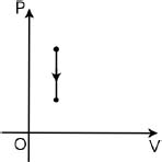
Figure 2.4:Isochoric process
Referring to Fig. 2.4, an isochoric or isovolumetric process is one in which the volume of the system does not change (i.e. dV = 0). Then,
By the first law of thermodynamics,


Figure 2.5:Isobaric process
Referring to Fig. 2.5, an isobaric process is a process in which the pressure of the system remains constant.
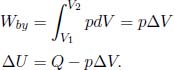
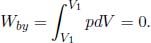
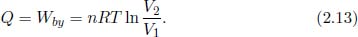
Reversible Isothermal Process

Figure 2.6:Isothermal process
Referring to Fig. 2.6, an isothermal process is one in which the temperature of the system remains constant.

An example of an isothermal process is the expansion of a cylinder of gas with a thin wall performed by pulling the piston extremely slowly, allowing sufficient time for the gas to gain heat through the container walls to constantly maintain thermal equilibrium with its surroundings. Furthermore, since  during an isothermal process. The first law of thermodynamics then implies that
Adiabatic Process

Figure 2.7:Adiabatic process
Referring to Fig. 2.7, an adiabatic process is a reversible (and thus necessarily quasistatic) process in which there is no net heat transfer between a system and its external surroundings (i.e. Q = 0).
Adiabatic processes usually involve well-insulated containers. An example would be the gradual increase in external pressure on a thermally insulated gas piston such that the pressure of the gas is always equal to the external pressure as it contracts. An example of a process that involves Q = 0 but is not adiabatic would be a sudden compression of a cylinder of gas performed by pushing the piston rapidly such that there is negligible time for heat to escape the system — this is not an adiabatic process as it is non-quasistatic and irreversible. To calculate the work done by the gas in an adiabatic process, we will use the following paramount adiabatic condition. In an adiabatic process,

where c is an arbitrary constant determined by initial conditions. γ is the adiabatic index and is given by

where f is the degrees of freedom of a gas molecule. As a corollary of this condition, adiabats drawn on a PV diagram are steeper than isotherms as  for an adiabat with γ > 1, as compared to
  for an isotherm.
Proof: The differential form of the first law of thermodynamics implies that

Since δQ = 0 for an adiabatic process and δWon = –pdV for a reversible process,
We know that

Taking the total derivative of the above,
Dividing the whole equation by  yields

Integrating the above and taking the exponential of both sides,

for some constant c. Observe that we have proven the adiabatic condition from the first law of thermodynamics and the ideal gas law. Therefore, if we are interested in analyzing a reversible adiabatic process involving a gas, we can simply use the adiabatic condition, instead of the first law of thermodynamics, in combination with the ideal gas law. The resultant equations are often simpler this way. Now, to determine the work done by the gas in a reversible adiabatic process, we write
Substituting 

Alternatively, we could have derived Wby from ΔU via the first law of thermodynamics. Since Q = 0,

We know that U is given by

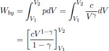
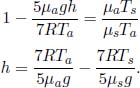
Problem: Burning a piece of wood releases smoke consisting of carbon monoxide (molar mass μs) at temperature Ts near the surface of the Earth. If the smoke then rises adiabatically (assume that there is no heat transfer between the atmosphere and the smoke), determine the maximum altitude h that the smoke can attain. The atmosphere can be presumed to have a uniform temperature Ta and molar mass μa. Furthermore,  , where g is the gravitational field strength near the surface of the Earth such that the density of atmospheric air can be assumed to be a constant up till altitude h.
The atmospheric pressure as a function of altitude h is approximately

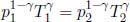
where p0 is the pressure at the surface and  is the uniform mass density of the atmosphere. For the smoke to undergo an adiabatic process, its pressure at all instances must be equal to p(h). By the adiabatic condition, the temperature of the smoke T(h) as a function of altitude obeys

Since  for a diatomic gas (carbon monoxide),

The smoke stops rising when its density is equal to that of the atmosphere ρa as the upthrust just balances its weight. This occurs when

Substituting the expression for p(h),
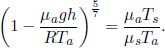
Since  , we can perform a binomial expansion to obtain
If a block of copper and a block of aluminium, that are initially at the same temperature and are of equal masses, are placed into identical beakers of water, the final temperatures of water in the two beakers, at thermal equilibrium, are different. Thus, we conclude that the two blocks must have stored different quantities of heat as internal energy even though they were initially at the same temperature. Therefore, it is natural to define a property that refers to the additional amount of heat required to raise the temperature of a substance by unit temperature as temperature on its own is not a good gauge of the internal energy of a substance. This quantity is known as the heat capacity C of the substance. Concretely,

where Q and T are the heat supplied to the system and the temperature of the system. Applying the first law of thermodynamics,

We see that if δWon = 0 throughout the thermodynamic process, dU = CdT such that C is a good measure of the internal energy stored by the substance. Most notably, we have

where Cv is the heat capacity of an isochoric process. Since the changes in volume of solids and liquids are often negligible throughout all types of processes (i.e.they are all approximately isochoric), we can simply define a heat capacity C for them that is process-independent (since dU = CdT for all processes and U is a state function). However, the value of C of a gaseous system, on the other hand, depends on the process as Won changes accordingly in Eq. (2.17). Thus, we need to define different values of C for different processes in a gaseous system. Furthermore, C is no longer a measure of the stored internal energy of a gas as part of the heat supplied could have been used as work done by the gas. Before we determine these for isochoric and isobaric processes, it is intuitive that a larger amount of a substance requires a greater quantity of heat for the same change in temperature as a larger system is basically a smaller system duplicated by several parts. It is then natural to define a property for the additional amount of heat required to increase the temperature of a substance by unit temperature, per amount of substance — this is known as the specific heat capacity of the substance. The amount of substance usually refers to the mass of substance m for solids and liquids and the number of moles of gas molecules n for gases. In the case of the latter, the specific heat capacity of gases with respect to the number of moles is known as the molar specific heat capacity. Quantitatively,
where c is the specific heat capacity. If c is independent of T,

Once again, we emphasize that the molar specific heat capacity of a gas varies across different processes. Therefore, it is convenient to calculate the molar specific heat capacities for specific processes — namely isochoric and isobaric processes. We will derive them for gases with a general number of degrees of freedom.
For an isochoric process, by Eq. (2.18),
In the case of a reversible isobaric process, δWon = –pdV and δQ = ncpdT by definition so

since pdV = nRdT by the ideal gas law under isobaric conditions,

where we have also shown that cv and cp are independent of temperature for an ideal gas.
We see that the molar specific heat capacity of a gas under constant pressure is larger than that under constant volume as work must be done by the gas (to expand when temperature increases). Quantitatively, cp = cv + R. Considering these expressions for cv and cp, the more general definition of the adiabatic index is in fact

Problem:When a constant power P is transferred to a solid, its temperature T increases according to
where t is the time elapsed and T0 is the initial temperature. Determine the heat capacity of the solid C(T) as a function of its temperature.

Enthalpy
It may be noteworthy that a state function known as the enthalpy H of a substance is defined as

where U, p and V are its internal energy, pressure and volume respectively. For our purposes, it is merely another state function, derived from other state functions, but chemists prefer to use it for the following reason. Observe that for a substance undergoing a reversible isobaric process,

where Cp is the heat capacity at constant pressure. Therefore,

where δQ is the heat absorbed by the substance during the reversible isobaric process. Since experiments on Earth are usually performed under constant pressure (atmospheric pressure), H is a more convenient pathway in specifying the heat absorbed by a substance. Finally, it can be seen that a stronger form of Eq. (2.23) holds for an ideal gas. Since U = ncvT and pV = nRT for an ideal gas, its enthalpy is

This implies that the relationship

is valid for any general process on an ideal gas of fixed moles, just as  .
.
In this section, we will explore how the first law of thermodynamics can be applied to situations where a gas enters or leaves a container. The interpretation of work done in such processes is often more subtle and is dependent of our definition of a system, as the following example shall illustrate.
Problem: In Fig. 2.8, an evacuated chamber is placed on the surface of the Earth where the pressure and temperature of atmospheric air — which can be presumed to be diatomic — are p0 and T0. If the cap sealing the chamber is opened, determine the temperature of the gas inside the chamber at the instance where there is no longer any net influx of air molecules into the chamber. The tank is insulated such that there is negligible heat transfer between the inside of the tank and the atmosphere. Assume that no air leaks out of the chamber once it has entered it.
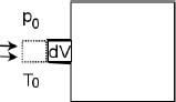
Figure 2.8:Evacuated chamber
Firstly, note that the relevant final temperature of the gas in the chamber is not necessarily T0, as the gas may not have attained thermal equilibrium with the atmosphere when a mechanical equilibrium is established (i.e. the final pressure of the gas is p0). Now, we reach a junction where we have to choose a system to apply the first law of thermodynamics to.
Method 1: Control Mass Just like what we have done in the previous sections, we can pick a set of gas molecules as our system and track them. This method is known as the control mass approach as we fix the constituents of our system. In the context of this problem, we can choose our system as the group of gas particles that will enter the chamber. The change in the macroscopic energies of this system is negligible and there is no heat transfer between the atmosphere and this system. The first law of thermodynamics then states that

Now, the origin of Won is rather subtle. Suppose the total volume of our system in the atmosphere is V0. As our control mass enters the chamber, its posterior experiences a pressure p0 which is analogous to a piston with pressure p0. Therefore, we can readily state

where n is the total number of moles of gas that enters the chamber and T0 is the atmospheric temperature as the piston pushes volume V0 of gas into the chamber. Note that the possible work done on the incoming back sections by the front sections which are already in the chamber is excluded precisely because we have defined all gas molecules that will eventually enter the chamber as our system, such that this component of work is not performed by an external agent. In other words, though the work done on the arriving section by the gas already in the chamber increases the internal energy of the arriving section, there is a corresponding decrease in the internal energy of the gas in the chamber and thus no net change in the internal energy of our system due to this factor. With this clarification, we proceed with substituting  for a diatomic gas. Hence,

The final temperature Tf is

Method 2: Control Volume Instead of choosing a predetermined group of particles as our system, we can demarcate a region known as a control volume and analyze the energies entering and leaving this region. In this case, we can define the control volume as the chamber. Let n now denote the instantaneous number of moles stored in the chamber. In a short time interval dt, the only change in energy inside the control volume stems from the dn moles of atmospheric molecules, which occupy volume dV in the atmosphere, entering the chamber. Since their macroscopic energies are negligible, the total energy carried by these molecules is their final internal energy which is their initial internal energy (internal energy in the atmosphere  ) plus the gain in internal energy due to the work done on them by the gas section immediately behind them as they are pushed in.
For purposes of illustration, suppose that the arriving gas section has a cross sectional area dA and a length dx. The force by the gas section at the back of this section on this section is p0dA and must have acted over a distance dx to push it into the chamber. Consequently, the work done on the arriving section by its posterior neighbour, which is known as flow work, is p0dV = dnRT0. Note that the meaning of this work is slightly different from Won afore. The p0V0 term in the previous method arose from the work done on all molecules that will enter the chamber by other atmospheric molecules. However, the p0dV term here indicates the work done on incoming gas molecules due to the gas molecules immediately behind them, which may or may not eventually enter the chamber. In a certain sense, we may be including the “internal forces” in our analysis. At this point, you may wonder why we did not consider the work done on the infinitesimal section dV entering the chamber due to the gas already inside the chamber. This is because, the incoming gas section becomes part of the system once it enters the control volume (chamber) — meaning that this does not represent a flow of energy outside of the control volume.
Moving on, the rate of increase of energy, which is manifested solely as internal energy U, inside our control volume is therefore

Integrating and substituting the initial values of U and n as zero,

where Uf and nf are the final internal energy and the number of moles of gas inside the chamber respectively. Since  where Tf is the final temperature,

Steady Flows
The control volume approach introduced afore presents a neat method of analyzing steady gas flows in which the properties of each point in a system do not vary with time. Recall that a streamline delineates the trajectory of a fluid molecule when the flow is steady. Now, consider the steady flow of a gas along a streamtube which consists of a bundle of adjacent streamlines. Suppose that we wish to relate the flow speeds (v), temperatures (T) and heights h at two points along a streamtube as shown in Fig. 2.9.

Figure 2.9:Streamtube
Let the rate of moles of gas molecules flowing through a cross section be  . This must be uniform through the entire streamtube at steady state and is equivalent to the mass continuity equation. Let the cross sectional areas of the right and left ends next to the demarcated region in the stream tube be A1 and A2 respectively. Then, the mass continuity equation is

where η represents the number density in a region, which can be computed as  by ideal gas law. Thus, the mass continuity equation is equivalent to stating that

Moving on, we also can exploit the fact that the energy of the region between these two points should be constant with respect to time at steady state. That is, we can balance the energy influx into and outflow from the demarcated region. In time dt, other than work done and heat transfer into the demarcated region by entities external to the streamtube, there is a change in energy within the region due to dn moles of molecules (with molar mass μ) entering from the left and dn moles of molecules exiting from the right. The net increase in macroscopic kinetic energy is  where v1 and v2 are the respective flow speeds while the net increase in gravitational potential energy is μdng(h1 – h2) (we assume that other forms of potential energy are absent). Meanwhile, the net increase in energy inside the dashed boundary due to the internal energies of the incoming and outgoing molecules is dncv(T1 – T2) + p1dV1 – p2dV2 where dV1 and dV2 are the volumes of the incoming and outgoing molecules at the respective ends. As for the last two terms, remember that we have to include the flow work done by the molecules behind the incoming molecules on the left end (which is positive) and that by the molecules in front of the outgoing molecules on the right end (which is negative as the force due to their pressure opposes the flow velocity v2). Since p1dV1 = dnRT1 and p2dV2 = dnRT2, the above can be rewritten as

where cp is the molar heat capacity at constant pressure. Another way to see this is that dncvT1 + p1dV1 and dncvT2 + p2dV2 are simply the enthalpies of the incoming and outgoing molecules, dncpT1 and dncpT2! All-in-all, the rate of change of energy in the demarcated region is

Most of the time, the rate of external heat flow  and work done
  are zero such that the above becomes

since  is uniform. Equivalently,

In words, the sum of the macroscopic kinetic and potential energies, the internal energy of the molecules and flow work performed by posterior molecules at any point along a streamtube is a constant. In cases where the potential energy term is also negligible, the conserved quantity is  . This quantity divided by cp is known as the stagnation temperature Tt.

Its physical meaning is the temperature at the point along the streamline that is stationary. Now, the term “stationary” implies that we need to specify a reference frame for its meaning to be unambiguous. Recall that we have assumed that the flow was steady when deriving the above equations. Therefore, the relevant point must be stationary relative to the frame in which the flow is steady and the streamlines do not move with time. Conversely, we can express the maximum macroscopic speed (when T = 0) that the gas can attain with respect to this frame as

Problem: A rocket in outer space propels itself by burning fuel to release diatomic gas of temperature T1 in its combustion chamber which has a cross sectional area A1. The gas then flows adiabatically and is expelled out of the nozzle, which has a cross sectional A2, at a speed v2 relative to the rocket and at pressure p2 and temperature T2 < T1. If the rocket is designed correctly (i.e. its cross sectional area is varied appropriately) such that steady flow relative to the rocket is achieved, determine the thrust experienced by the rocket.
We will analyze this set-up in the frame of the rocket. Let the pressure of the released gas at the combustion chamber be p1 and let it have a speed v1 relative to the rocket. Firstly, the adiabatic condition implies that
where  for a diatomic gas.

Since the flow is steady in the frame of the rocket, mass continuity (Eq. (2.27)) requires

Substituting the expression for p1 in terms of p2,

Applying Eq. (2.29) while neglecting the change in gravitational potential energy,

where μ is the molar mass of the diatomic gas. Substituting the expression for v1 in terms of v2,

The rate of moles of molecules exiting the nozzle is  where η2 is the number density of gas molecules at the nozzle. As such, after a time interval dt, the momentum of the gas molecules that escape in the frame of the rocket is

Observe that after this time interval dt, the total momentum of the gas flowing in the rocket increases by dp in the frame of the rocket. Therefore, by the conservation of momentum, the rocket’s momentum must have changed by –dp. Therefore, the thrust experienced by the rocket is

where the negative sign indicates that the force is opposite in direction to the relative velocity of the ejected gas.
This section will discuss the microscopic perspective to ideal gases in classical thermodynamics by modeling a system as a large collection of discrete molecules. Only monoatomic molecules with no rotational and vibrational modes will be considered. In the limit where the volume of the system tends to infinity with a constant density — an ideal known as the thermodynamic limit — thermal fluctuations are smoothed out such that thermodynamic quantities are close to their average values. Quantitatively, taking the average of N independent samples of a variable yields a standard deviation that is  times the standard deviation of a single sample. Since the standard deviation is a natural measure of the spread or uncertainty of a distribution, the decrease in standard deviation with N causes thermal fluctuations to be negligible, as N in this context refers to the number of molecules in a system, which is gargantuan. This notion also sheds light on the statistical nature of thermodynamics which involves probabilistic laws that are accurate in the regime of many constituents.
Velocity Distribution Function
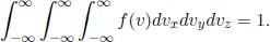
A velocity distribution function f(v) = f(vx, vy, vz) is used to describe the fraction of molecules with a velocity in the immediate vicinity of a certain v, just like any other probability distribution function. Concretely, it is a three-dimensional probability distribution function (one for each spatial dimension) such that the fraction of molecules with velocities between v = (vx, vy, vz) and (vx + dvx,vy + dvy, vz + dvz) is f(v)dvxdvydvz.
Since the motion of gas molecules is proposed to be isotropic, the velocity distribution function should only be dependent on speed and not the direction of velocity.

Given this isotropic nature, a common mistake is to assume that the fraction of molecules traveling at speeds between v and v + dv and whose velocities make an angle between θ and θ + dθ with a fixed axis, such as the z-axis, is equal for all θ. This confusion is best rectified by considering the velocity space, in Fig. 2.10, which is a sphere that depicts the possible velocities of the molecules as vectors extending from the origin.

Figure 2.10:Molecules with angles between θ and θ + dθ
Since every point in velocity space represents a velocity, the velocity distribution function can be ascribed to every point in space to quantify the fraction of molecules possessing that particular velocity per unit volume around that point. Due to the isotropic nature of the distribution, this probability density is uniform over a spherical shell at a constant radius (and thus constant speed) away from the origin. Observe that the fraction of molecules travelling at speeds between v and v + dv that make an angle between θ and θ + dθ with respect to the z-axis is an approximately circular hoop of radius v sin θ, width vdθ and thickness dv (spherical coordinates). Then, the relevant fraction is 2πv2f(v) sin θdθdv which is non-uniform across different θ for a given speed.
Finally, the velocity distribution function needs to be normalized like any other probability distribution function. This can be evaluated in Cartesian coordinates and also conveniently, in spherical coordinates due to its isotropy.


Speed Distribution Function
The distribution of the speeds of molecules can be easily computed from the velocity distribution. Since the velocity distribution is uniform for a constant speed v, the fraction of molecules having a speed between v and v + dv is simply the volume of a spherical shell of radius v and thickness dv, multiplied by f(v). The speed distribution function fs(v) is then

and is a one-dimension distribution. Then, the fraction of molecules with speeds between v and v + dv and velocities that make an angle between θ and θ + dθ with a certain axis can be expressed as

Finally, note that if f(v) is normalized, fs(v) is also normalized as a result of Eq. (2.32).
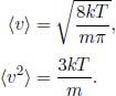
We have now covered the two important distribution functions in kinetic theory. Do not worry about the exact functions for now as this will be discussed in a later section. Instead, let us focus on how thermodynamic variables can be described in terms of these distributions. However, we will still be using the following results for the mean, mean square and mean cube speeds which are consequences of the speed distribution:
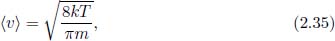
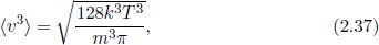
where k is the Boltzmann constant, T is the temperature of the gas and m is the mass of a single molecule.
Collisions with a Stationary Area
We first analyze the rate of collisions of molecules per unit area with a stationary wall. Consider an infinitesimal area dA and define the positive z-axis to be parallel to its area vector (which is pointing outwards from the container). We will adopt spherical coordinates in this problem. Firstly, we consider molecules that travel at a particular speed v. The volume swept by molecules with velocity v that subtends an angle θ with respect to the z-axis in time dt is of the shape in Fig. 2.11.

Figure 2.11:Volume of molecules with velocity v that collide with the wall in time dt
The shape has a total volume of

By Eq. (2.34), the number of collisions with the area dA in time dt due to this particular class of molecules is thus  , where η is the number density of molecules which is assumed to be uniform. Therefore, the number of collisions per unit area, per unit time due to molecules that travel at speeds between v and v + dv and angles between θ and θ + dθ is

Momentum Transfer Per Collision
When a molecule traveling at speed v and angle θ collides with the stationary wall, it rebounds and effectively reverses its velocity in the z-direction, assuming that the collision is elastic. Therefore, the momentum transferred to the infinitesimal area is 2mv cos θ in the positive z-direction. The pressure contribution dp due to molecules traveling between speeds v and v + dv and angle θ and θ + dθ is then the momentum transferred per collision multiplied by the number of collisions per unit area, per unit time.

The total pressure on the wall is then obtained by integrating the above over all relevant v and θ. Note that θ is only integrated from 0 to  as only molecules travelling in the positive z-direction are germane.
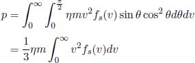
where 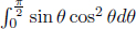 can be solved via the substitutions u = cos θ, du = –sin θdθ. Now, observe that the final integral averages v2 to produce the mean square speed. Thus,
which is often written as  where ρ = ηm is the mass density of the gas. Substituting the expression for
  in Eq. (4.7), we can prove the ideal gas equation.

where N is the total number of molecules.
Effusion is the process where gas molecules escape from a small hole of area A and a diameter smaller than the mean free path of the molecules — the average distance traveled by the molecules between consecutive collisions. Interesting effusion properties to compute would be the molecular flux out of the hole and the rate of change of internal energy of the gas remaining in the container. The speed distribution of escaped molecules is also intriguing and shall be deferred to a later section. For now, we should understand qualitatively that the speed distribution of effused molecules favors molecules with higher speeds (as compared to the standard speed distribution fs(v)) as these molecules are more energetic and more likely to escape from the hole.
Equation (2.38) is the rate of molecules of speeds between v and v+dv and angles between θ and θ + dθ colliding with a stationary wall, per unit area, and is similarly, also the rate of molecules effusing out of a small hole, per unit area. After integration over the relevant range of θ (this does not change the expression’s dependence on v), the (instantaneous) speed distribution fe(v) of escaping molecules is proportional to vfs(v). It can be seen from the additional factor of v, as compared to fs(v), that effusion preferentially selects molecules with greater speeds as they are more likely to escape from the hole.
Next, the molecular flux, which is the rate of moles of gas flowing out of the hole, can be calculated by multiplying Eq. (2.38) by A and integrating over the relevant limits.

The above can be expressed solely in terms of the thermodynamic properties p and T by substituting  and by expressing η in terms of p and T via the ideal gas law:

Therefore,

Since Φ is inversely proportional to  , effusion can be used to separate different gas molecules and isotopes of the same gas. As the lighter molecules effuse at a greater rate, the preponderance of molecules left in the container will be the heavier molecules.
Problem: Effusion is often applied in uranium enrichment processes. Suppose that we have a large sample of two different isotopes of uranium trapped in two different gas molecules of molar masses μ1 and μ2 > μ1. Initially, the ratio of molecules with molar mass μ1 to those of molar mass μ2 is q < 0.5. We can purify a sample of homogeneous temperature by allowing it to effuse through a membrane fraught with porous holes that have diameters smaller than the mean free path of the molecules and collecting the molecules that pass through the filter up till a period of time. Backwards effusion is negligible. Determine the number of cycles needed to increase the previous ratio to at least 2q by repeatedly applying this procedure.
Suppose that the ratio of molecules with molar masses μ1 to those with μ2 is r currently. Since  , the ratio of the rates of effusion is

The new ratio after a single step is evidently

Therefore, the minimum number of stages required to increase the ratio to at least 2q is
Next, it is useful to determine the rate of energy loss engendered by the escaping molecules. Equation (2.38) is the rate of molecules with speed v and angle θ escaping the hole, per unit area. Therefore, the total kinetic energy by this class of particles, that escape the hole, can be determined by multiplying Eq. (2.38) by mv2 (kinetic energy of a molecule of that class) and A, and integrating over the relevant limits.

where E is the total internal energy remaining in the container. Substituting  ,
,
The average energy of an effusing molecule can be determined by dividing the magnitude of the rate of energy lost by the molecular flux.

which is evidently more than the average kinetic energy of a molecule originally in the container,  kT.
kT.
In this section, we will model the collisions between gas molecules and determine the mean free time and mean free path which are the average time elapsed and distance covered between consecutive collisions of a molecule. Important assumptions in this model are that colliding molecules are scattered elastically in random directions after a collision and that collisions between different time intervals are independent events.
Monoatomic gas molecules are modeled as hard spheres with a radius r. Suppose that we select a particular particle and follow its motion. Then, observe that the tracked molecule can collide with another molecule if the center of the other molecule is within a circular cross section of radius 2r from the center of the tracked molecule, as shown in Fig. 2.12.

Figure 2.12:Effective collision radius
Therefore, we define the effective collision cross sectional area as
Now, let the tracked particle have a constant velocity v until its next collision and define u to be the velocity of a particular class of other molecules that it could collide with. Then in time dt, the effective collision volume swept by the tracked particle, relative to this class of molecules, is

The probability of a collision occurring between the tracked molecule and the particular class of molecules during the time interval, is the above multiplied by the number density of that particular class of molecules, f(u)ηduxduyduz.

Integrating the above over all u would yield the probability of the tracked molecule colliding in the time interval dt. Then, we can average the resultant expression over all v (all possible tracked molecules) to determine the probability of a molecule colliding in the time interval dt on average. This probability is

where vr is the relative speed between molecules. The average is performed over all possible v and u. Now, define P(t) as the probability that a molecule, on average, has not collided from time t = 0 to time t. Then, from the first principles of calculus,

Since the collision events during different time intervals are independent, the probability of a molecule surviving till t + dt is the product of the probability it survives till t and the probability of it not colliding in the interval between t and t + dt. This applies to the average case as well.

Comparing the two expressions for P(t + dt),

where the lower limit of P has been set to one as the probability that a molecule, on average, survives till t = 0 is one. Therefore,

Now, we can use the above to calculate the mean time between collisions. The probability of a molecule surviving till time t and colliding between the time interval from t to t + dt, on average, is simply the product of the probability that it survives till time t and the probability of it colliding within the time interval dt.

Therefore, the mean free time is obtained by multiplying the above by t and integrating over all t.

It can be shown that the average relative velocity  is exactly
  from the velocity distribution of gas molecules. The proof is non-trivial and will not be presented here. Following from this,
Substituting 

It can be seen that heavier molecules collide less frequently and that the mean collision interval is shorter for a larger temperature — both properties make intuitive sense. Following from this, the mean free path is
Macrostates and Microstates
A thermodynamics system can be described in two ways. Firstly, it can be quantified on the whole in terms of the macroscopic properties it exhibits such as temperature and pressure. These are the attributes measured during experiments. A set of such variables is known as a macrostate. Next, we can adopt another perspective by describing a system based on the parameters of all its constituents (e.g. by labeling all particles with their positions and velocities). A configuration consisting of such parameters is known as a microstate. Crucially, several microstates can result in the same macrostate. For example, suppose that you roll two dice — a possible macrostate may be the sum of the two numbers. Consider the particular sum 4 — it can be formed in three ways: 1 + 3, 2 + 2 and 3 + 1 which are different microstates of the system.
Boltzmann Distribution
Consider a system coupled to another gargantuan system, known as a heat reservoir, such that energy can be exchanged. The reservoir is so large that any heat extracted from or deposited into it does not vary its temperature significantly. If the system is in thermal equilibrium with the reservoir such that the common temperature is T, the probability of the system undertaking a microstate S with a certain energy E is proportional to e  , which is known as the Boltzmann factor.

Assume that there is only a single microstate corresponding to a single energy such that the probability can be expressed as a function of the energy of the system instead. If there are N microstates with the ith state having energy Ei, the probability of the system adopting the kth microstate with energy Ek is hence

Let us apply this to the simplest example of a two-state system with energy levels 0 and E. Then, the probability of each microstate is

We can also calculate the average energy as

Another intriguing application of the Boltzmann distribution pertains to an isothermal atmosphere with molar mass μ and uniform temperature T. By balancing forces on each gas section, one can obtain from basic mechanics that the pressure p(h) at a small altitude h above the surface of Earth obeys

where p0 is the pressure at the surface. An alternate perspective can be adopted by considering the distribution of molecules as a function of altitude. Since the gravitational potential energy per molecule at altitude h is mgh where m is the mass of a single molecule (the reference point has been set at the surface of the Earth), the Boltzmann distribution implies that the density ρ(h) of the atmospheric molecules varies with altitude h according to

where ρ0 is the density at the surface of Earth. Multiplying the numerator and denominator of the exponent by the Avogadro’s number NA,

Since  for an ideal gas,

Maxwell–Boltzmann Distributions
The Boltzmann distribution can be applied to a single ideal gas molecule by considering all other gas molecules as the heat reservoir. The resultant distributions (for velocity and speed) are known as the Maxwell–Boltzmann distributions. In this process, we are making the assumptions that there are no intermolecular forces and that the intermolecular distances are large as compared to the mean free path (average distance between consecutive collisions) of molecules, such that collisions occur once in a blue moon. These can be satisfied in the case of a very dilute gas. Then, we can approximately say that the system (which is one gas particle) is at equilibrium with a reservoir (all other particles), maintained at a temperature T.
In the case of a monoatomic molecule with only translational freedoms, its total energy (excluding possible macroscopic energies) is given by

where the x, y and z-directions are arbitrarily chosen. Then, the probability of a molecule having a velocity v between (vx, vy, vz) and (vx + dvx, vy + dvy, vz + dvz) is proportional to the Boltzmann factor. Since the molecules are assumed to be identical, the distribution of molecules having velocity v is identical to the probability distribution of the velocity of a single molecule. That is, a single molecule is representative of the entire system of molecules as they are identical. Then, the fraction of molecules having velocity v, f(v), is also proportional to the Boltzmann factor.

where A is a normalization factor. Note that we have already used the isotropic nature of the distribution to conclude that f is strictly a function of speed and independent of the direction of velocity. Now, we can evaluate A by imposing the condition that
Before this, let us go through a few integration tricks.
Integration Trick: Differentiating a Parameter
We shall discuss a general method for evaluating integrals of the form  and
and  where α is a constant and n is a non-negative integer. Firstly, we begin with the integral

Consider a second integral  where y is a variable independent of x. Due to this independence, the product of these integrals can be evaluated by combining their integrands.

These limits of integration are tantamount to the entire xy-plane. Therefore, the above can also be computed in terms of polar coordinates by substituting x = r cos θ and y = r sin θ. Then,

where we have also conveniently proven that  . Since Ix = Iy,

Now, notice that the integral above is a function of α.
Then, we can take the total derivative of this integral with respect to α.

Since α is independent of x which is the variable that we are integrating with respect to, the derivative can be moved within the integral.
Note that the total derivative becomes a partial derivative in the second expression as the integrand is also a function of x. We already know the exact expression for I(α), which is given by  such that
  . Then,

We can repeat this differentiation process to further evaluate expressions of the form  in general.

for n ≥ 1. Finally, in cases where we wish to compute  observe that the integrand is an even function such that
  .
.
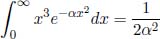
Next, to evaluate4  , we start from

In a similar vein, we can differentiate the above with respect to α within the integral to conclude that
and in general,

Normalization
Returning to the previous velocity distribution, we require

These are integrals of the form  which can be evaluated to be
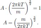
Then, the velocity distribution function is

It is convenient to express the above in terms of the thermal speed of gas molecules,  , whose physical meaning is the most probable speed of the gas molecules as we shall prove later.

Distribution of a Component of Velocity
Next, we can derive the one-dimensional distribution of a particular component velocity such as vx. That is, we are interested in the fraction of molecules with a particular x-component of velocity vx — molecules with different components in the other directions but the same component in the x-direction still belong to the same class. We argue that the components of velocity of the particles — namely vx, vy and vz — should be independent variables as the different components of velocity should be uncorrelated. Then, the fractional density of the particles attaining a velocity v between (vx, vy, vz) and (vx + dvx, vy + dvy, vz + dvz) is the product of the respective fractional densities.

where g(vi) is the distribution along a particular component. Apportioning the different variables (i.e. we put all functions of vx into g(vx), functions of vy into g(vy) and so on) and normalizing yields

and so on for the other directions.
Speed Distribution
The speed distribution is

We shall now prove that vth is the most probable speed (i.e. the maximum of fs(v)). Consider the derivative of fs(v) with respect to v.

For this to be zero,

where the physically incorrect negative solution has been rejected. Finally, one can check that the value of  is positive for values of v slightly smaller than vth and negative for values of v slightly larger than vth to show that this corresponds to a maximum. Moving on, fs(v) is graphed for two values of T in Fig. 2.13.
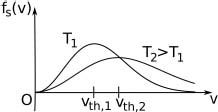
Figure 2.13:Maxwell–Boltzmann speed distribution
fs(v) is zero at v = 0, has a maximum and tends to zero as v tends to infinity. For larger values of T, the distribution becomes broader but the peak value decreases as the area under the curve must still be unity. The peak also shifts towards the right for larger values of T as vth increases. From the Maxwell–Boltzmann speed distribution, the mean and mean square speeds can be computed as
This is an important result (but do not overrate its significance) as it relates the temperature of an ideal gas to its mean squared speed. The mean translational kinetic energy is then related to the temperature according to

The mean cube speed can also be shown to be

Problem: Determine the speed distribution fe(v) of molecules effused from a small hole in a compartment given that the distribution of the original gas in the compartment is Maxwellian and that the compartment is maintained at a constant temperature T.
We have previously remarked that fe(v) is proportional to vfs(v) and thus  . Therefore,

for some constant A. Normalizing the distribution requires

Since we have calculated that 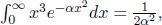

1.Real and Ideal Gas Thermometers*
A constant volume gas thermometer is constructed from connecting a gas chamber of a fixed volume to a manometer. The difference Δh in liquid levels in the manometer reflects the pressure of the gas in the chamber and the temperature T of the gas can then be read off a pre-calibrated linear graph between Δh and T. To measure the temperature of a substance (usually a liquid), the gas chamber is immersed in the substance such that its temperature becomes the temperature of the substance (the heat capacity of the gas is negligible). Now, a certain constant volume gas thermometer contains one mole of a gas whose equation of state is
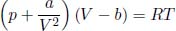
where a and b are characteristic constants of the gas. This is known as the van der Waals equation of state and is commonly used to model real gases. Another constant volume gas thermometer contains one mole of an ideal gas which obeys the ideal gas law, pV = RT. The thermometers are calibrated at the ice and steam points to give centigrade scales. Show that the two thermometers will give identical readings when placed in thermal contact with a substance of any temperature.
2.Connected Vessels*
Two thermally insulated vessels of volumes V1 and V2 initially contain monoatomic gases of initial pressures and temperatures p1, T1 and p2, T2. They are then linked by a thermally insulated tube. Determine the final pressure p and temperature T.
3.Isobaric Compression*
A certain amount of helium is cooled at constant pressure p0. As a result, its volume decreases from V0 to  . Find the amount of heat lost in this process.
4.Balloon*
A helium balloon is allowed to rise to a height such that the external pressure is half of the ground pressure p1. Its initial volume and temperature are V1 and T1 respectively. Assume that the envelope of the balloon is a perfect insulator and that the process is quasistatic. Calculate the final volume and temperature of the gas and the amount of work done by the gas. (Singapore Physics Olympiad)
5.Cyclic Process*
The current pressure and volume of an ideal gas are p0 and V0. It then undergoes a cyclic process as follows. It first expands under the constraint that  . Then, its pressure is reduced isochorically from 2p0 to p0. Finally, it contracts isobarically until its volume returns to V0. Determine the heat absorbed during this cyclic process.
6.Pushing a Piston*
A thermally insulated container of cross sectional area A is separated into two compartments, A and B, by a frictionless divider which is a perfect insulator. Certain moles of an ideal gas with an adiabatic constant γ fill the two compartments. A massless, thermally insulated piston at one end of compartment B is initially maintained at some pressure p. Initially, the system is at equilibrium such that volumes of A and B are  Al and
  Al. The pressure on the piston is then increased so gradually that the system is always at equilibrium, until the combined volume of the two compartments becomes Al′. If the temperature increments in the two compartments are ΔTA and ΔTB respectively, determine the number of moles of ideal gas they contain, nA and nB.
7.Moving a Division**
A gas-tight, thermally isolated cylinder of total volume V is divided into two compartments A and B by a piston made of a conducting material, which can be controlled by an external agent outside the cylinder. Initially, A and B are of equal volume; they contain respectively 1 and 2 moles of an ideal monoatomic gas, all at temperature T0 (the external agent holds the piston in place). The external agent then moves the piston to a position such that A and B possess final volumes  and
and  respectively. This is done sufficiently slowly for the temperatures of the two gas samples to remain uniform and equal throughout the process. Find an expression for the final temperature of the system while neglecting the heat capacity of the cylinder and piston.
8.Pumping a Balloon**
A balloon with surface tension γ (be wary that this is not the adiabatic index) is placed in a vacuum chamber and connected via a small tube to a gas container with a piston. The total number of moles of gas in the balloon and piston is n. The system is allowed to equilibrate such that the pressure of the gas in the combined system is p0. If the system is maintained at a constant temperature T and the pressure on the piston is quasistatically varied — such that the system is always at thermodynamic equilibrium — until all gas molecules in the piston are transferred to the balloon, determine the amount of work done on the gas by the piston. The final pressure of the gas is p1. Assume that the balloon constantly maintains a spherical shape.

9.Water Tap**
A container is partially filled with an ideal gas (on top) and incompressible water of density ρ. The initial pressure of the gas is 2pa where pa is the atmospheric pressure. If the small hole of area A of the bottom of the container is opened such that water begins to flow out of the container, determine the time required for the water to stop flowing if the ideal gas undergoes an isothermal process such that nRT = k where k is a constant. Assume that the flow of water is energy conserving and steady and neglect any difference in pressure due to the height of the water. The velocity of water inside the container is also negligible. Assume that the temperature of the water remains constant as well.
10.Pumping a Tyre**
A thermally insulated container with a movable, massless piston is connected to a thermally insulated tyre of constant volume V via a thermally insulated tube. During each pumping cycle, the valve in the tube is first closed. Then, the piston is expanded until the pressure and volume of the gas becomes pa and Va, by taking in air from the outside. The gas in the piston, which has an adiabatic index γ, is then compressed adiabatically until its volume becomes  . Finally, the valve is opened until equilibrium is reached between the container and the tyre. If the tyre does not contain any gas initially, determine the minimum number of cycles required to increase the pressure in the tyre to 2γ–1pa.
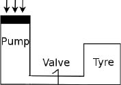
11.Rotating Gas**
An open container, exposed to the atmosphere, contains water of density ρw. An “L-shaped” tube is inserted into it as shown in the figure below. The diameter of the vertical part of the tube is negligible while the horizontal part of the tube has a uniform cross sectional area and length l. Initially, the tube is motionless such that the water level is completely flat at equilibrium. Subsequently, the tube is rotated at a constant angular velocity ω about the vertical column such that the water level in the tube is a height Δh above the water level in the container at equilibrium. If the atmospheric pressure and temperature are pa and T and if the molar mass of the gas inside the tube is μ, determine Δh. Assume that the gas in the tube undergoes an isothermal process and  where R is the ideal gas constant.
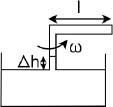
12.Adiabatic Oscillation**
A small cork of cross sectional area A and mass m blocks the opening of a wine bottle that is filled with an ideal gas with an adiabatic constant γ. If the atmospheric pressure is p0 and the volume of gas inside the bottle is V0 at the equilibrium state, determine the angular frequency of small oscillations of the cork about its equilibrium position.

13.Bouncing Ball**
A thermally insulated container with a constant cross sectional area A is separated into an upper and lower compartment by a divider of mass M. The two compartments are filled with certain moles of ideal gas which can exchange heat with one another as the divider is not thermally insulated. A small ball of a certain mass m is stuck to the bottom face of the divider. Initially, the ratio of the volumes of the upper and lower compartments is 3 : 1 and the pressure of the gas in the upper compartment is p1. Then, the ball of mass m falls from the divider and bounces on the bottom of the container, until it eventually comes to rest at the bottom of the lower compartment. If the final ratio of the volumes of the upper and lower compartments is 2 : 1, determine m.
14.Dumping Water***
An inverted container with a constant cross sectional area and mass m is floating with its base at the water level as shown in the figure below. The height of the air column is h0. The plate holding back the water on top is then removed such that water falls down at negligible velocity — causing the instantaneous depth of the container, which is defined to be the distance between the water level and the base of the container, to become h1. The column of air between the two water sections dissolves and has no impact on the system. Argue qualitatively that the container should sink. If the entire set-up has a constant temperature T and the gas in the container instantaneously attains thermodynamic equilibrium at every depth of the container, determine the velocity of the container at depth h (assume that  is small). Neglect atmospheric pressure. Now, interpret your results for h0 → 0.

Gas Flows
15.Combining Flows*
Two tubes carrying an identical ideal gas flowing at pressures p1, p2 and temperatures T1, T2 merge at a junction into a combined third tube. If the flow velocities at all parts of the tubes are negligible and if the volume flow rate in the first tube is k times that of the second tube, determine the temperature T3 of the gas exiting from the third tube. The flow is and the tubes are thermally insulated.
16.Sustaining a Fan*
A fan of cross sectional area A steadily takes in diatomic air molecules of molar mass μ, pressure p1 and temperature T1 and expels it at velocity v2, pressure p2 and temperature T2. Determine the electric power needed to sustain the fan (assuming that it is perfectly efficient).
17.Speed of Sound**
This problem will explore an elegant way of deriving the speed of a onedimensional sound wave in a gaseous medium:  where γ, p and ρ are the adiabatic index, ambient pressure and density of the gaseous medium. Suppose that the sound wave travels adiabatically in the x-direction at velocity c and that the currently oscillating point along the medium travels at a small velocity –v (v
  c) in the lab frame. The density of the currently oscillating section only differs from the ambient pressure by a small amount Δρ ρ. Think of a way to apply the equations describing steady flow (mass and energy continuity). Through these two equations and the adiabatic condition, you will obtain two equations that are linear combinations of two variables (one of which is v) that are equated to zero. By exploiting the fact that the determinant must be zero for the two variables to have non-trivial solutions, determine c.
Kinetic Theory of Gases
18.Pressure*
Prove Eq. (2.39) by considering molecules traveling at a particular z-component of velocity vz. You will have to relate  to
to  . (Note that we did not use this simple proof in order to expedite the derivation of Eq. (2.40).)
19.Equipartition Theorem*
Suppose that the energy of a system in a particular state, quantified by the variable x which can range from –∞ to ∞, is E = αx2 where α is a constant. If the probability of the system adopting a certain state follows the Boltzmann distribution, show that the average energy of the system is  , where k is the Boltzmann constant and T is the temperature of the system. If the energy of the system in a particular state is now E =
  , where the
  are independent variables that collectively define a state and each ranges from –∞ to ∞, show that the average energy is given by
  .
.
20.Equilibrating Effusion*
A container is separated into two compartments of volumes V1 and V2 by a massive divider. The first compartment initially contains n0 moles of an ideal gas while the other compartment is empty. If a hole, with a diameter smaller than the mean free path of molecules, is made on the divider and the two compartments are maintained at temperatures T1 and T2, determine the pressure in each compartment when the system has equilibrated.
21.Isothermal Leaking**
A hole of area A, whose diameter is smaller than the mean free path of gas molecules, is punctured on the surface of a container of volume V that rests in a vacuum. If the initial number density of ideal gas molecules inside the container is η0 and the gas is constantly in a state of equilibrium, determine the number density η(t) if the gas is maintained at a constant temperature T and if each molecule has mass m. Then, determine the external power supplied to the gas inside the cylinder. Neglect all form of energy loss, other than that due to the escaping molecules.
22.Thermal Conductivity**
This problem concerns estimating the thermal conductivity of an ideal gas via the kinetic theory of gases. By Fourier’s law of conduction, the heat flux density, or the power delivered per unit perpendicular area, across an area is proportional to the temperature gradient.

where the z-direction has been set as the direction along which temperature varies, q is the heat flow per unit area — implying that  is the power per unit area. The negative sign in the above equation implies that heat flows from regions of higher temperature to regions of lower temperature. Finally, k is the thermal conductivity which we aim to determine in this problem.
Now, consider the following set-up. Two large plates parallel to the xy-plane are located at certain z-coordinates. They are maintained at different temperatures such that a steady, position-dependent temperature T(z), that is strictly decreasing with increasing z, is set up in the region between them. An ideal gas with f degrees of freedom fills this region.
(a)Argue qualitatively why there will be power delivered across a plane of a constant z-coordinate based on the varying temperature T(z).
(b)It is known that the gas molecules have a mean free path λ. Now, consider a class of gas molecules with a certain velocity that makes an angle θ with the z-direction. If the gas molecules cut across a plane of z-coordinate z at a particular instance, what is the average kinetic energy carried by them?
(c)Using the previous result, determine the heat flux density and thermal conductivity k across a plane of z-coordinate z, in terms of the degrees of freedom of the gas molecules f, the number density η (assumed to be uniform throughout), λ and the average speed  of the gas molecules at a plane of z-coordinate z. Assume that λ is small such that second order and above terms in λ are negligible.
23.Adiabatic Condition***
Through the kinetic theory of gases, show that a process involving a monoatomic ideal gas in a thermally insulated container with a slowly moving and thermally insulated piston conserves the quantity  where T and V are the instantaneous temperature and volume respectively. The speed of the piston is very small as compared to the speed of the gas molecules. Assume that the collisions between the gas molecules and the piston are perfectly elastic.
24.Leaking Container***
A hole of area A, whose diameter is smaller than the mean free path of gas molecules, is made on a thermally insulated container of volume V, that is placed in a large vacuum. If the initial number density of gas molecules inside the container is η0 and the initial temperature is T0, show that the number density η(t) obeys
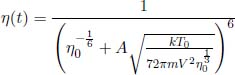
where m is the mass of one molecule. Assume that the gas inside the container constantly attains a homogeneous equilibrium state. Hint: consider the rate of change of number density and the internal energy of the gas inside the container.
1.Real and Ideal Gas Thermometers*
Since V is constant, observe that both equations of state imply a linear relationship between p and T. For the van der Waals gas,
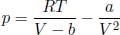
while for the ideal gas,

Since the height difference Δh between the two liquid levels in a manometer is proportional to the difference between the pressure of the gas and the (constant) atmospheric pressure, the above implies that Δh obeys a linear relationship with T for both gases.

Since the calibration itself is used to fit a linear relationship between Δh and T and because we know that the actual relationship between Δh and T is indeed linear for both gases, both thermometers will correctly reflect the real temperature of the substance measured. The readings are then naturally the same.
2.Connected Vessels*
Since the vessels are thermally insulated, the total internal energy must beconserved.  for an ideal gas. Therefore,

Next, the total number of moles is

The final temperature is then

3.Isobaric Compression*
Let the initial and final temperatures of the gas be T0 and T1 respectively. By the ideal gas law,

The heat transferred to the gas in the process is then

where the negative sign indicates heat loss by the gas.
4.Balloon*
Let the final volume and temperature be V2 and T2 respectively. By the adiabatic condition,

since γ =  for a monoatomic gas (helium). By the ideal gas law,
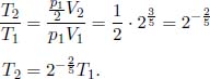
By the first law of thermodynamics, during an adiabatic process,
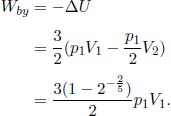
5.Cyclic Process*
The PV curve of the process is a right-angled triangle with side lengths p0 and V0. Therefore, the work done by the gas (the reader should check for the sign) is

The internal energy of the gas remains the same after the process as the initial and final states are the same. Then, by the first law of thermodynamics, the heat absorbed by the gas is

6.Pushing a Piston*
At each intermediate stage of the process, the system is in an equilibrium state such that the pressures in the two compartments are equal. Furthermore, since the walls are insulated, the gases in the two compartments undergo adiabatic processes. Let  and VB be the respective initial and final volumes of the gases in the compartments. If the final common pressure is p′,

Dividing the first equation by the second, it can be seen that the ratio of the volumes of the compartments remains the same. That is,  and
and  . By substituting one of these expressions into the corresponding equation above,

Applying the ideal gas law to the gas in compartment A,
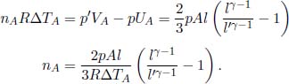
Similarly,
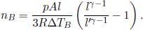
7.Moving a Division**
An important point to note in this problem is that the pressures of the two gases need not be equal at any instance in time (even when thermal equilibrium has been attained) as the forces on the piston can always be balanced by the external agent. Let VA be the instantaneous volume of compartment A. If the external agent moves the piston such that VA is changed to VA + dVA at this instance, the work done by the external agent on the system comprising the two gases is (PB – PA)dVA, where PA and PB are the respective pressures of the gases in compartments A and B. In writing this, we have noted that the change in volume of the gas in B must be –dVA. By the work-energy theorem, the work done by the external agent must be equal to the increase in internal energy of the two gases,  , where T is the instantaneous common temperature of the gases.

Substituting  and
and 

8.Pumping a Balloon**
The total work done by a gas in an isothermal process is given by Eq. (2.13). Therefore, the total work done on the gas is

since pV is constant for an isothermal process. This is not work done by the piston on the gas, Wpiston, on, as the balloon also performs work on the gas, Wballoon, on.
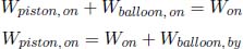
where Wballoon, by is the work done on the balloon by the gas. This is equal to the negative change in surface energy of the balloon. Recall that the surface energy of a spherical balloon is 4πγr2 where r is the radius of the balloon. Let the initial and final radii of the balloon be r0 and r1 We know that

due to the pressure discontinuity caused by surface tension across the surface of a spherical balloon at equilibrium. Solving the above for r0 and r1 in terms of the respective pressures, the change in surface energy is
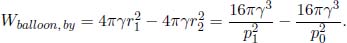
Therefore,

Another method in evaluating the work done by the piston on the gas would be to evaluate – directly, with V being the volume of gas in the gas piston. Let the instantaneous pressure of the gas and the radius of the balloon be P and r. Since the gas is at equilibrium at every instance,

Furthermore, by the ideal gas law,
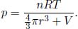
Substituting the expression for r in terms of p, obtained from the first equation, into the second equation,

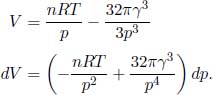
The work done on the gas by the piston is then

9.Water Tap**
Let the instantaneous pressure and volume of the gas be p and V. Then, p and V are related by

Next, let v be the velocity of water gushing out of the hole. Applying Bernoulli’s principle5 to the water level and the hole,

The volume flow rate of water is Av. This is also the rate of increase of the volume of the gas,  .
.

Substituting  ,
,
The initial and final volumes are  and
and  . Then,
To evaluate the left-hand side, use the substitutions  and
and  . Then,
Then, the time required is

10.Pumping a Tyre**
Let the final pressure of the gas after the adiabatic compression be  . Then by the adiabatic condition,

We have shown in a previous problem that when two thermally insulated vessels of initial pressures and volumes p1, p2, V1 and V2 are connected, the final pressure is

Let us apply this result to the current problem. Let the pressure inside the tyre after the ith cycle be pi. Then, the equilibrium pressure after the (i+1)th cycle is that obtained by connecting two thermally insulated vessels of initial pressures and volumes  and V. Then,

The above can be simplified into
It can be seen that the above is a geometric progression with a constant ratio  the base case p0 = 0,
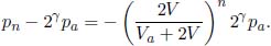
When 
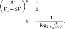
The minimum number of cycles is the ceiling of the above value.
11.Rotating Gas**
Firstly, understand that when the tube is rotated, the pressure p(r) in the tube must vary as a function of radial distance r from the axis of rotation to provide the centripetal force required by each gas section to remain at rest relative to the tube. As a consequence of the ideal gas law, the density ρ(r) of the gas must also vary with radial distance. Consider an infinitesimal section of gas between radial distance r and r + dr. It has a mass density ρ(r) and we define its cross sectional area to be A. Therefore, its mass is dm = ρAdr. The external forces on this element are pA radially outwards and (p + dp)A radially inwards. The net force must provide the required centripetal force.
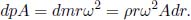
Then,

Furthermore, we know from the ideal gas law that
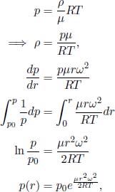
where p0 is the pressure at radial distance r = 0 (i.e. along the axis of rotation). Now, our objective is to determine p0 as its difference with the atmospheric pressure enables us to compute Δh via the pressure difference caused by a static column of fluid. To this end, we can exploit the fact that the total mass of gas in the tube must be the same as before. That is,

where ρ0 is the uniform density of gas before the tube was rotated.

Substituting  , the above requires

This difference in pressure causes the water to rise up the tube until
12.Adiabatic Oscillation**
At the equilibrium position, the pressure of the gas inside the wine bottle is  so the net force due to pressure balances the weight of the cork. Now, consider a small displacement x upwards, such that the new volume of the gas is

Let the pressure of the gas at this point be p. Applying Newton’s second law to the cork,

If the oscillations are small and thus slow (by the conservation of energy), the process that the gas in the bottle undergoes is adiabatic. In an adiabatic process, the quantity pVγ is a constant. Therefore,

Performing a binomial expansion on the denominator and discarding second order terms in  ,
,

The angular frequency of oscillations is thus

13.Bouncing Ball**
Let the initial pressures in the upper and lower compartment be p1 and p2. Let the final pressures be  and
and  . In order for the system to be in mechanical equilibrium, the pressure differences must balance the pressure due to the weight of the piston (and the weight of the ball in the first case).
Next, we know that gases must have common initial and final temperatures. Then, the ratio of moles in the two compartments are given by the ideal gas law as

Substituting  and the expressions for p2 and in terms of p1 and ,

Next, we can apply the conservation of energy to this system. The decrease in gravitational potential energy of the ball must be equal to the increase in the internal energies of the gases and the gravitational potential energy of the divider. Equivalently, the falling ball supplies heat to the system during the collisions. If we let the total volume of the container be V0,

Simplifying,

Equating the two expressions for would yield a quadratic equation in m.


where we have rejected the other solution which is negative.
14.Dumping Water***
Before the water falls onto the container, the upthrust is just enough to balance the weight of the container. However, when water is dumped onto the container, the pressure of the gas inside the container should increase — causing it to contract under isothermal conditions. This results in a shrinking volume of gas and thus a smaller value of upthrust — causing the container to sink further. This propagates a vicious cycle as the more the container sinks, the higher the pressure of the gas and the smaller the upthrust — thus causing it to sink even further.
Let us now try to solve for the velocity of the container  as a function of its depth h. Let the density of water be ρ and the cross sectional area of the container be A. Initially, the upthrust must balance the weight of the container.

Under isothermal conditions, the quantity pV is conserved. The initial pressure of the gas is  and the initial volume is Ah0 Therefore, the conserved quantity is

Now, we aim to calculate the height of the air column x at thermodynamic equilibrium when the depth of the container is h. The pressure and volume of the gas at this juncture are then ρg(h + x) and Ax. Then,
Since 

where we have rejected the negative solution. Performing a binomial expansion and neglecting higher order terms in  ,
,

Now, apply Newton’s second law to the container — the external forces on it are its weight and the upthrust.

Expressing  as
as  and separating variables,

where we have removed the absolute value brackets for the ln term as h > h1. Then,
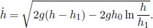
When h0 → 0,

which is just the velocity of a free-falling particle (as there is no upthrust when h0 = 0). Technically, this limit is slightly incorrect as the container should not have been able to stay afloat before the water was dropped.
15.Combining Flows*
Suppose that in time dt, dn1 and dn2 moles of gas molecules enter the junction from the first and second tubes respectively. By mass continuity, the number of moles leaving the third tube in this time interval must be dn1 + dn2. One can now enforce the continuity of energy flow across the junction, similar to the section on gas flows, to show that

Since  and
and 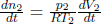 where
where  and
and  are the volume flow rates in the respective tubes. Dividing the previous equation by dt and substituting these,
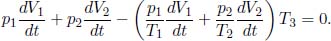
Since 

16.Sustaining a Fan*
By Eq. (2.27), mass continuity requires

where v1 is the flow velocity entering the fan as the cross sectional area A is common for both sides of the flow.

Note that the molar flow rate is

Applying Eq. (2.28) with  , the rate, work done by the fan on the gas flowing through it is

Substituting  for a diatomic gas and

which is also the power required to sustain the fan.
17.Speed of Sound**
Since the sound wave propagates at velocity c in the x-direction, the pressure and density should be constant with time in a frame that travels at c in the x-direction relative to the lab frame — implying that the flow is steady. In this new frame, the speed of the oscillating section is c + v while the speed of the sections that are not oscillating is c. Enforcing mass continuity,

Furthermore, by Eq. (2.29) and neglecting the gravitational potential energy terms,
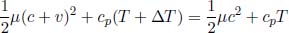
where μ and cp are the molar mass and isobaric molar heat capacity of the medium. T is the ambient temperature and T + ΔT is the temperature of the oscillating section. Discarding terms that are second order in v or Δρ in the above equations,
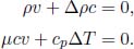
ΔT can be related to Δρ through the adiabatic condition. Since  constant and
  by the ideal gas law,

for some constant c. Taking the total derivative of the above,
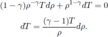
Since Δρ and ΔT are small,

Substituting this expression for ΔT and summarizing our equations,

The above set of equations can be written in matrix form as

For non-trivial solutions to exist for v and Δρ, the determinant of the first matrix must be zero.

Notice that  and
and  by the ideal gas law such that the above becomes

18.Pressure*
Consider an infinitesimal area dA and define the z-axis to be parallel to its area vector. Consider a class of molecules that are travelling at z-component of velocity vz. In time dt, the volume of such molecules colliding with the area is

The number of such molecules colliding the infinitesimal area, per unit time and area is then

where η is the number density of molecules and g(vz)dvz is the fraction of molecules with z-components of velocity between vz and vz + dvz. The elastic collision of one of such molecules with the wall results in 2mvz amount of momentum transferred to the wall. The pressure on the wall due to this class of molecules is then the rate of such molecules colliding with the wall, per unit area, multiplied by the momentum transferred per molecule. The total pressure is then obtained by integrating the above over all classes of molecules (i.e. vz from 0 to ∞).
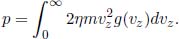
Note that the integral 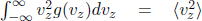 — implying that
  . Then,

Now, we need to relate  to
to  .
.
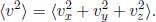
Since the different components of velocities are independent,

Moreover, the three directions are symmetrical such that 

19.Equipartition Theorem*
By the Boltzmann distribution, the probability of attaining a state x which has energy αx2 obeys the relationship
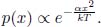
Therefore, the average energy is

where integrals of the form  and
and  have been computed previously. In the second scenario, the probability of attaining a state
  which has energy
  is
is
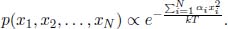
The average energy is therefore
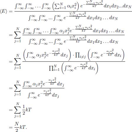
20.Equilibrating Effusion*
The effusion rate is proportional to  where p and T are the pressure and temperature of the gas. Let the pressures of the compartments at equilibrium be p1 and p2. Then,

Note that the pressure on both sides are not necessarily equal for an equilibrium to be attained as we just have to ensure that there is no net transfer of molecules. Moving on, the total number of molecules must be conserved.

Solving the two equations above,

21.Isothermal Leaking**
From the effusion equation,
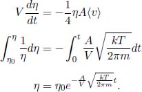
To compute the power supplied to the container, we can subtract the total rate of change of internal energy of the gas by the rate of kinetic energy lost by the escaped molecules. The latter is given by Eq. (2.42) as
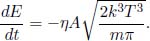
The former can be obtained by differentiating  . Since V and T are constant,

Therefore, the external power is
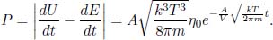
22.Thermal Conductivity**
(a)Consider a plane of a certain z-coordinate z. In time dt, some molecules on the bottom and top of this plane crosses the plane. Since the bottom region possesses a higher temperature, more molecules on the bottom cross the plane than those on the top and they carry a larger kinetic energy with them. Then, there will be a net energy transfer from the bottom to the top, across the plane at z-coordinate z.
(b)The molecules crossing the plane at coordinate z would have, on average, traveled a distance λ since their last collision. Therefore, the molecules traveling at an angle θ with respect to the z-axis would have traveled a distance λ cos θ in the z-direction on average and are representative of the temperature T(z – λ cos θ) as their kinetic energies do not change until their next collisions. The average kinetic energy of such molecules is then

where we have used kb to denote the Boltzmann constant to avoid confusion with the thermal conductivity k.
(c)Now, consider the net energy change due to one molecule with speed v and angle θ leaving the plane at z and due to one molecule arriving with speed v and angle θ, with temperature T(z – λ cos θ). The net energy change due to the exchange of one such pair of molecules is

Next, we know from Eq. (2.38) that the fraction of molecules with speed v and angle θ crossing the plane, per unit area and time, is  . Therefore, the heat flux density is obtained by multiplying this by
 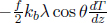 and integrating over all relevant v and θ. Note that the limits of θ are from 0 to π as we want to encompass molecules from both above and below the plane of z-coordinate z. However, by combining these into a single integral, we are assuming that the temperature variation is small across distances in orders of λ as fs(v) would change across different z-coordinates. Including such variations would result in second order terms in λ in the expression for the heat flux density which will be discarded anyway. Therefore, we can integrate over all relevant limits with a constant fs(v), taken to be the speed distribution at coordinate z.
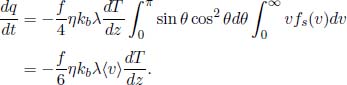
Therefore, the thermal conductivity is approximately

where  is the average speed at z-coordinate z.
23.Adiabatic Condition***
Consider an infinitesimal area dA on the piston and define the positive x-direction to be parallel to its area vector. Let the velocity of this area be u. The number of molecules with an x-component of velocity vx colliding with this area in time dt is
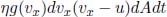
where η is the number density of molecules and g(vx)dvx is the fraction of molecules with an x-component of velocity between vx and vx + dvx. The energy change in the gas due to collisions with the piston can be computed by observing that the final x-component of velocity of a gas molecule is (vx – 2u) in the reverse direction after a collision. Therefore, if the mass of a molecule is m, the change in energy due to one collision is
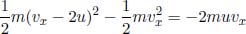
where we have discarded the second order term in u. Therefore, the change in internal energy of the ideal gas due to the collision between this class of molecules with the infinitesimal area dA is

Then, the total change in internal energy is obtained by integrating the above over all classes of molecules and all areas on the piston. In the case of the latter, we are essentially integrating udAdt over the surface of the piston which results in an infinitesimal change in volume dV. Thus, the total change in energy is

Since 

where v is the speed of a molecule and the angle brackets represent taking the mean of. Next, since the internal energy E of a gas is simply the total microscopic kinetic energy,

Substituting this into the expression for dE,
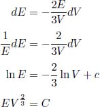
for some constant C. Next, E is proportional to  and thus T (by the Boltzmann distribution). We can also state that E is proportional to T directly by the equipartition theorem which is actually a consequence of the Boltzmann distribution. Exploiting E ∝ T, the quantity
  must be conserved.
24.Leaking Container***
From the effusion equation, we know that
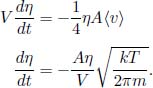
From Eq. (2.42), the total rate of change of internal energy is

Now, we need to solve the system of equations comprising  and
and  . In this process, we note that T is a variable as the more energetic molecules are favored in escaping the container — causing the average energy of the molecules remaining in the container to decrease with time. Hence, we first express everything in terms of E and η to eliminate T. Since

From the two equations above,

where  is the initial energy We let the right-hand side be c for the sake of convenience. Since
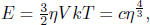

Substituting this expression for T into  ,
,

Solving this differential equation by separating variables would yield the desired result.
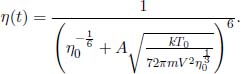
1Vibrational degrees of freedom are not included here as the energies associated with them are not quadratic in a certain variable. They are in fact quantized.
2The speed in the context of polyatomic molecules would usually refer to the speed of the center of mass.
3This concept of reversibility will be explored in the next chapter.
4Note that it is meaningless to determine  , which is just zero as the integrand is an odd function.
5The reader may wonder if Bernoulli’s principle is valid in this context, especially after perusing the section on gas flows. In our derivation of Bernoulli’s principle, the possible change in the internal energy of a fluid was excluded. In the current situation, this does not matter as the temperature of the water is uniform and because water is presumed to be incompressible.