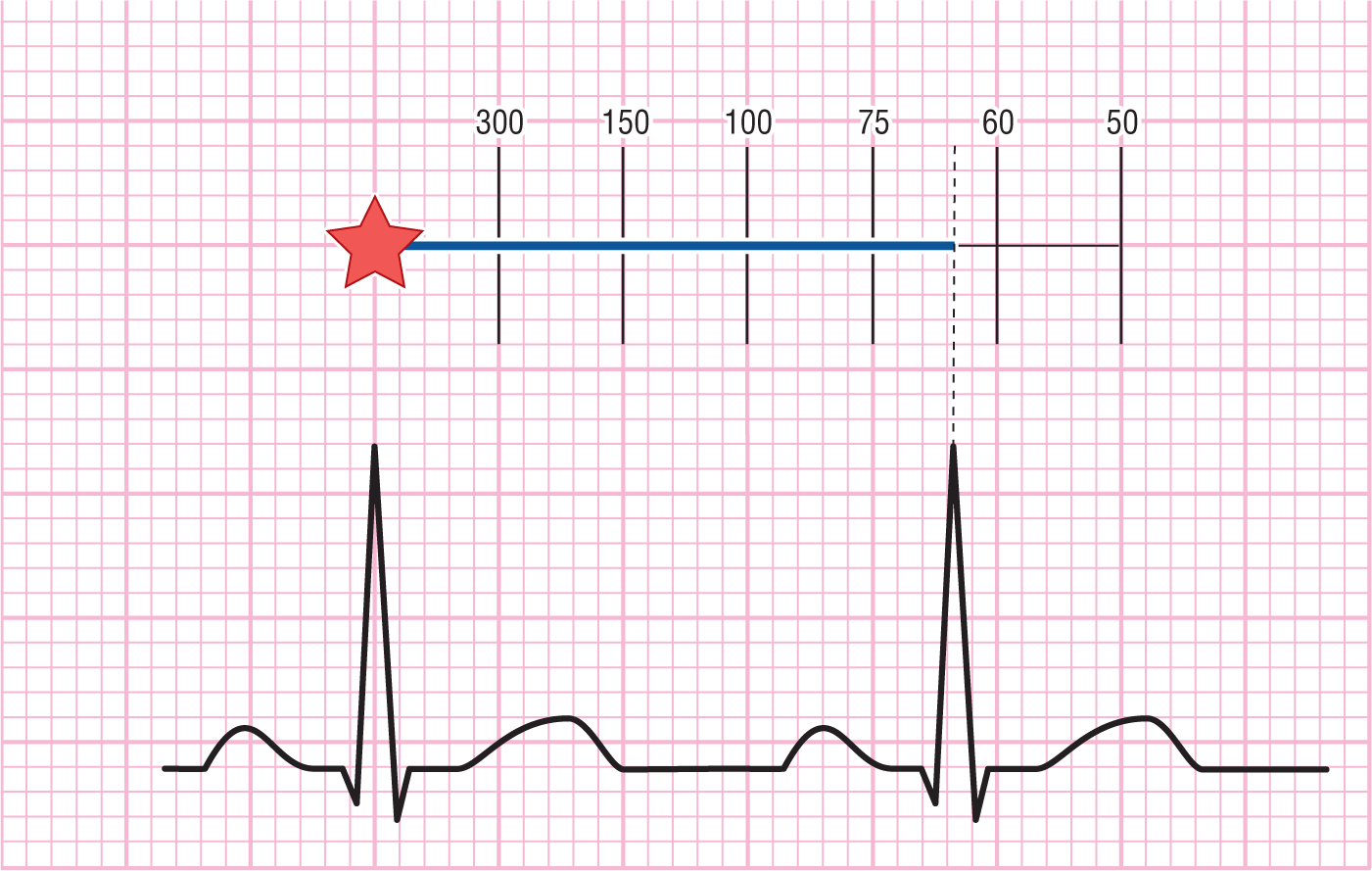
Figure 3-12 The rate is approximately 65–70 BPM.
© Jones & Bartlett Learning.
DescriptionThe easiest way to calculate the rate is to use the method illustrated in Figure 3-12. Find a QRS complex that starts on a thick line; this will be your starting point (Figure 3-13). Next, go to the exact spot on the next QRS complex—your end point. By tradition, we try to use the tip of the tallest wave on the QRS complex. However, you can use any spot as long as it is consistent. Then just count the thick lines in between the two spots, using the numbers shown in Figure 3-12. You will have to memorize this sequence, but it is more than worth your trouble.
Figure 3-12 The rate is approximately 65–70 BPM.
© Jones & Bartlett Learning.
Description
REMINDER
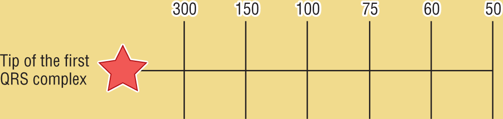
Figure 3-13 These are the rates corresponding to thick lines following the tip of the QRS complex that lands on (or is adjusted to, using calipers) an initial thick line.
© Jones & Bartlett Learning.
Another way to calculate the rate is to use your calipers to measure from the top of one complex to the top of the next. Then move the calipers—maintaining the measured distance—so that the left tip rests on a thick line, and calculate the rate as above for the distance between the two tips. The advantage here is that you don’t have to hunt down a QRS that lands on a thick line to use as a starting point.
Do you remember the concept in Figure 3-14? Knowing these time intervals will be very useful when you are calculating bradycardic rhythms. Can you think of how to use these intervals to calculate the rate generally, but especially in irregular and slow rhythms?
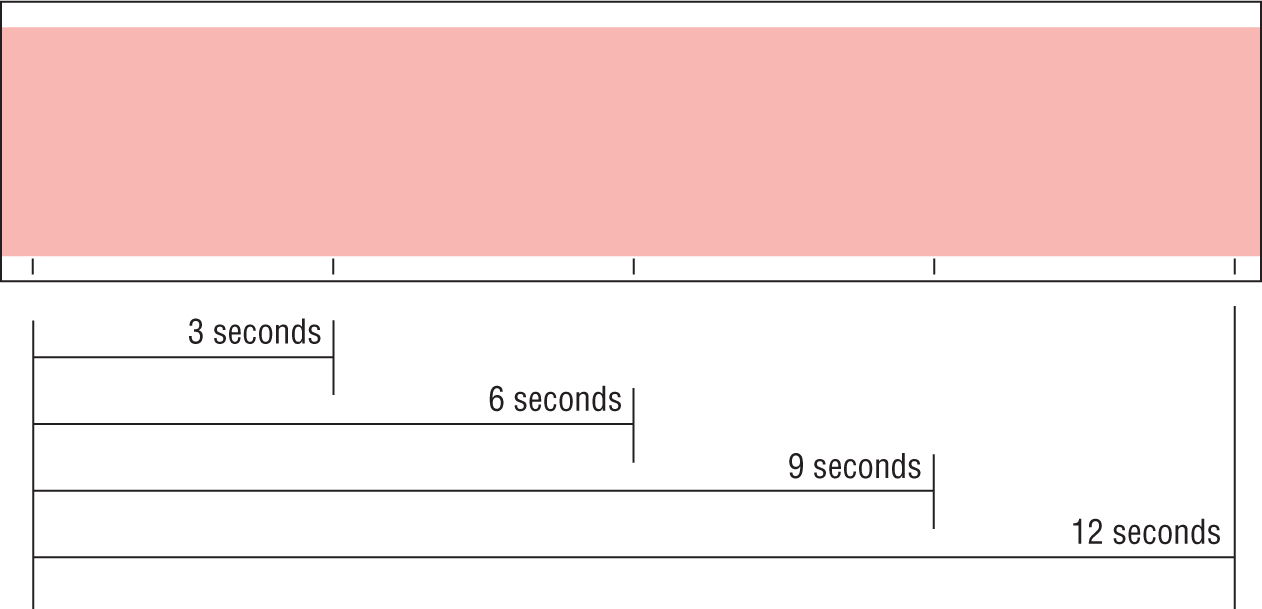
Figure 3-14 ECG paper.
© Jones & Bartlett Learning.
REMINDER
(cycles in 6 sec.) × 10 5 BPM
It’s simple. Just count the number of cycles present in a 6-second strip, and multiply that number by 10. This will give you the number of beats in 60 seconds. You could also count the number of cycles in a 12-second strip and multiply by 5. Remember to use the fractional parts of cycles in your calculations, for example, 3.5 cycles in 6 seconds gives a rate of 35 beats per minute (3.5 cycles × 10 = 35 BPM). For examples, see Figures 3-15 and 3-16.