 NOTE Chapter 12 continues the hard drive discussion by adding in the operating systems, showing you how to prepare drives to receive data, and teaching you how to maintain and upgrade drives in Windows.
In this chapter, you will learn how to
• Explain how hard drives work
• Identify and explain the PATA and SATA hard drive interfaces
• Identify and explain the SCSI hard drive interfaces
• Describe how to protect data with RAID
• Install hard drives
• Configure CMOS and install drivers
• Troubleshoot hard drive installation
Of all the hardware on a PC, none gets more attention—or gives more anguish—than the hard drive. There’s a good reason for this: if the hard drive breaks, you lose data. As you probably know, when the data goes, you have to redo work or restore from a backup—or worse. It’s good to worry about the data, because the data runs the office, maintains the payrolls, and stores the e-mail. This level of concern is so strong that even the most neophyte PC users are exposed to terms such as IDE, PATA, SATA, and controller—even if they don’t put the terms into practice.
This chapter focuses on how hard drives work, beginning with the internal layout and organization of hard drives. You’ll look at the different types of hard drives used today (PATA, SATA, SSD, and SCSI), how they interface with the PC, and how to install them properly into a system. The chapter covers how more than one drive may work with other drives to provide data safety and improve speed through a feature called RAID. Let’s get started.
Hard drives come in two major types. The most common type has moving parts; the newer and more expensive technology has no moving parts. Let’s look at both.
NOTE Chapter 12 continues the hard drive discussion by adding in the operating systems, showing you how to prepare drives to receive data, and teaching you how to maintain and upgrade drives in Windows.
A traditional hard disk drive (HDD) is composed of individual disks, or platters, with read/write heads on actuator arms controlled by a servo motor—all contained in a sealed case that prevents contamination by outside air (see Figure 11-1).
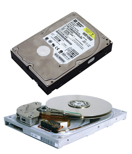
Figure 11-1 Inside the hard drive
The aluminum platters are coated with a magnetic medium. Two tiny read/write heads service each platter, one to read the top and the other to read the bottom of the platter (see Figure 11-2).
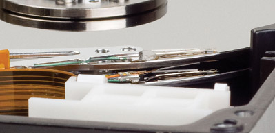
Figure 11-2 Read/write heads on actuator arms
The coating on the platters is phenomenally smooth. It has to be, as the read/write heads actually float on a cushion of air above the platters, which spin at speeds between 3500 and 15,000 RPM. The distance (flying height) between the heads and the disk surface is less than the thickness of a fingerprint. The closer the read/write heads are to the platter, the more densely the data packs onto the drive. These infinitesimal tolerances demand that the platters never be exposed to outside air. Even a tiny dust particle on a platter would act like a mountain in the way of the read/write heads and would cause catastrophic damage to the drive. To keep the air clean inside the drive, all hard drives use a tiny, heavily filtered aperture to keep the air pressure equalized between the interior and the exterior of the drive.
Although the hard drive stores data in binary form, visualizing a magnetized spot representing a one and a non-magnetized spot representing a zero grossly oversimplifies the process. Hard drives store data in tiny magnetic fields—think of them as tiny magnets that can be placed in either direction on the platter. Each tiny magnetic field, called a flux, can switch north/south polarity back and forth through a process called flux reversal. When a read/write head goes over an area where a flux reversal has occurred, the head reads a small electrical current.
Today’s hard drives use a complex and efficient method to interpret flux reversals. Instead of reading individual flux reversals, a modern hard drive reads groups of them called runs. Starting around 1991, hard drives began using a data encoding system known as run length limited (RLL). With RLL, any combination of ones and zeros can be stored in a preset combination of about 15 different runs. The hard drive looks for these runs and reads them as a group, resulting in much faster and much more densely packed data.
Current drives use an extremely advanced method of RLL called Partial Response Maximum Likelihood (PRML) encoding. As hard drives pack more and more fluxes on the drive, the individual fluxes start to interact with each other, making it more and more difficult for the drive to verify where one flux stops and another starts. PRML uses powerful, intelligent circuitry to analyze each flux reversal and make a “best guess” as to what type of flux reversal it just read. As a result, the maximum run length for PRML drives reaches up to 16 to 20 fluxes, far more than the 7 or so on RLL drives. Longer run lengths enable the hard drive to use more complicated run combinations so the hard drive can store a phenomenal amount of data. For example, a run of only 12 fluxes on a hard drive might equal a string of 30 or 40 ones and zeros when handed to the system from the hard drive.
The size required by each magnetic flux on a hard drive has reduced considerably over the years, resulting in higher capacities. As fluxes become smaller, they begin to interfere with each other in weird ways. I have to say weird because to make sense of what’s going on at this subatomic level (I told you these fluxes are small!) would require you to take a semester of quantum mechanics. Let’s just say that laying fluxes flat against the platter has reached its limit. To get around this problem, hard drive makers began to make hard drives that store their fluxes vertically (up and down) rather than longitudinally (forward and backward), enabling them to make hard drives in the 1 terabyte (1024 gigabyte) range. Manufacturers call this vertical storage method perpendicular recording.
For all this discussion and detail on data encoding, the day-to-day PC technician never deals with encoding. Sometimes, however, knowing what you don’t need to know helps as much as knowing what you do need to know. Fortunately, data encoding is inherent to the hard drive and completely invisible to the system. You’re never going to have to deal with data encoding, but you’ll sure sound smart when talking to other PC techs if you know your RLL from your PRML!
The read/write heads move across the platter on the ends of actuator arms or head actuators. In the entire history of hard drives, manufacturers have used only two technologies to move the arms: stepper motor and voice coil. Hard drives first used stepper motor technology, but today they’ve all moved to voice coil.
NOTE Floppy disk drives used stepper motors.
Stepper motor technology moved the arm in fixed increments or steps, but the technology had several limitations that doomed it. Because the interface between motor and actuator arm required minimal slippage to ensure precise and reproducible movements, the positioning of the arms became less precise over time. This physical deterioration caused data transfer errors. Additionally, heat deformation wreaked havoc with stepper motor drives. Just as valve clearances in automobile engines change with operating temperature, the positioning accuracy changed as the PC operated and various hard drive components got warmer. Although very small, these changes caused problems. Accessing the data written on a cold hard drive, for example, became difficult after the disk warmed. In addition, the read/write heads could damage the disk surface if not parked (set in a non-data area) when not in use, requiring techs to use special parking programs before transporting a stepper motor drive.
All magnetic hard drives made today employ a linear motor to move the actuator arms. The linear motor, more popularly called a voice coil motor, uses a permanent magnet surrounding a coil on the actuator arm. When an electrical current passes, the coil generates a magnetic field that moves the actuator arm. The direction of the actuator arm’s movement depends on the polarity of the electrical current through the coil. Because the voice coil and the actuator arm never touch, no degradation in positional accuracy takes place over time. Voice coil drives automatically park the heads when the drive loses power, making the old stepper motor park programs obsolete.
Lacking the discrete steps of the stepper motor drive, a voice coil drive cannot accurately predict the movement of the heads across the disk. To make sure voice coil drives land exactly in the correct area, the drive reserves one side of one platter for navigational purposes. This area essentially maps the exact location of the data on the drive. The voice coil moves the read/write head to its best guess about the correct position on the hard drive. The read/write head then uses this map to fine-tune its true position and make any necessary adjustments.
Now that you have a basic understanding of how a drive physically stores data, let’s turn to how the hard drive organizes that data so we can use that drive.
Have you ever seen a cassette tape? If you look at the actual brown Mylar (a type of plastic) tape, nothing will tell you whether sound is recorded on that tape. Assuming the tape is not blank, however, you know something is on the tape. Cassettes store music in distinct magnetized lines. You could say that the physical placement of those lines of magnetism is the tape’s “geometry.”
Geometry also determines where a hard drive stores data. As with a cassette tape, if you opened up a hard drive, you would not see the geometry. But rest assured that the drive has geometry; in fact, every model of hard drive uses a different geometry. We describe the geometry for a particular hard drive with a set of numbers representing three values: heads, cylinders, and sectors per track.
Heads The number of heads for a specific hard drive describes, rather logically, the number of read/write heads used by the drive to store data. Every platter requires two heads. If a hard drive has four platters, for example, it needs eight heads (see Figure 11-3).
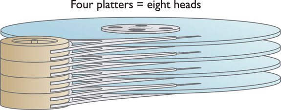
Figure 11-3 Two heads per platter
Based on this description of heads, you would think that hard drives would always have an even number of heads, right? Wrong! Most hard drives reserve a head or two for their own use. Therefore, a hard drive can have either an even or an odd number of heads.
Cylinders To visualize cylinders, imagine taking an empty soup can and opening both ends. Look at the shape of the can; it is a geometric shape called a cylinder. Now imagine taking that cylinder and sharpening one end so that it easily cuts through the hardest metal. Visualize placing the ex-soup can over the hard drive and pushing it down through the drive. The can cuts into one side and out the other of each platter. Each circle transcribed by the can is where you store data on the drive, and is called a track.
Each side of each platter contains tens of thousands of tracks. Interestingly enough, the individual tracks themselves are not directly part of the drive geometry. Our interest lies only in the groups of tracks of the same diameter, going all of the way through the drive. Each group of tracks of the same diameter is called a cylinder (see Figure 11-4). There’s more than one cylinder. Go get yourself about a thousand more cans, each one a different diameter, and push them through the hard drive.
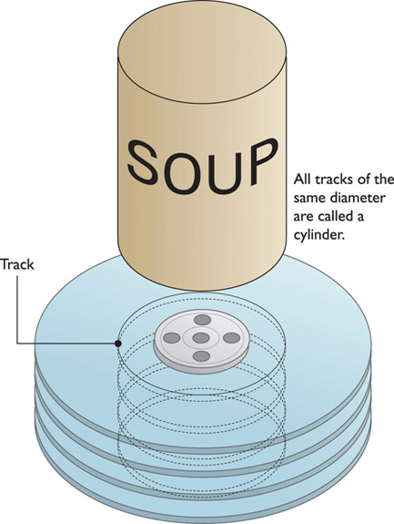
Figure 11-4 Cylinder
Sectors per Track Now imagine cutting the hard drive like a birthday cake, slicing all of the tracks into tens of thousands of small slivers. Each sliver then has many thousands of small pieces of track. The term sector refers to a specific piece of track on a sliver, and each sector stores 512 bytes of data.
The sector is the universal atom of all hard drives. You can’t divide data into anything smaller than a sector. Although sectors are important, the number of sectors is not a geometry value that describes a hard drive. The geometry value is called sectors per track (sectors/track). The sectors/track value describes the number of sectors in each track (see Figure 11-5).
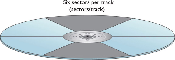
Figure 11-5 Sectors per track
The Big Three Cylinders, heads, and sectors/track combine to define the hard drive’s geometry. In most cases, these three critical values are referred to as CHS. The three values are important because the PC’s BIOS needs to know the drive’s geometry to know how to talk to the drive. Back in the old days, a technician needed to enter these values into the CMOS setup program manually. Today, every hard drive stores the CHS information in the drive itself, in an electronic format that enables the BIOS to query the drive automatically to determine these values. You’ll see more on this later in the chapter, in the “Autodetection” section.
Two other values—write precompensation cylinder and landing zone—are no longer relevant in today’s PCs. People still toss around these terms, however, and a few CMOS setup utilities still support them—another classic example of a technology appendix. Let’s look at these two holdouts from another era so when you access CMOS, you won’t say, “What the heck are these?”
Write Precompensation Cylinder Older hard drives had a real problem with the fact that sectors toward the inside of the drives were much smaller than sectors toward the outside. To handle this, an older drive would spread data a little farther apart once it got to a particular cylinder. This cylinder was called the write precompensation (write precomp) cylinder, and the PC had to know which cylinder began this wider data spacing. Hard drives no longer have this problem, making the write precomp setting obsolete.
Landing Zone On older hard drives with stepper motors, the landing zone value designated an unused cylinder as a “parking place” for the read/write heads. As mentioned earlier, before moving old stepper motor hard drives, the read/write heads needed to be parked to avoid accidental damage. Today’s voice coil drives park themselves whenever they’re not accessing data, automatically placing the read/write heads on the landing zone. As a result, the BIOS no longer needs the landing zone geometry.
Hard drives run at a set spindle speed, measured in revolutions per minute (RPM). Older drives ran at a speed of 3600 RPM, but new drives are hitting 15,000 RPM. The faster the spindle speed, the faster the controller can store and retrieve data. Here are the common speeds: 5400, 7200, 10,000 and 15,000 RPM.
Faster drives mean better system performance, but they can also cause the computer to overheat. This is especially true in tight cases, such as minitowers, and in cases containing many drives. Two 5400-RPM drives might run forever, snugly tucked together in your old case. But slap a hot new 15,000 RPM drive in that same case and watch your system start crashing right and left!
You can deal with these very fast drives by adding drive bay fans between the drives or migrating to a more spacious case. Most enthusiasts end up doing both. Drive bay fans sit at the front of a bay and blow air across the drive. They range in price from $10 to $100 (U.S.) and can lower the temperature of your drives dramatically. Some cases come with a bay fan built in (see Figure 11-6).
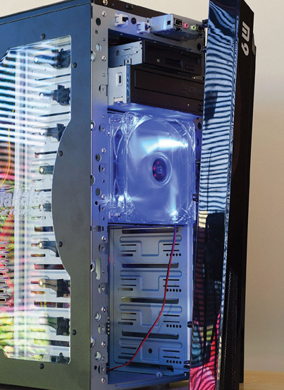
Figure 11-6 Bay fan
Airflow in a case can make or break your system stability, especially when you add new drives that increase the ambient temperature. Hot systems get flaky and lock up at odd moments. Many things can impede the airflow—jumbled-up ribbon cables, drives squished together in a tiny case, fans clogged by dust or animal hair, and so on.
Technicians need to be aware of the dangers when adding a new hard drive to an older system. Get into the habit of tying off ribbon cables, adding front fans to cases when systems lock up intermittently, and making sure any fans run well. Finally, if a client wants a new drive for a system in a tiny minitower with only the power supply fan to cool it off, be gentle, but definitely steer the client to one of the slower drives!
Booting up a computer takes time in part because a traditional hard drive needs to first spin up before the read/write heads can retrieve data off the drive and load it into RAM. All of the moving metal parts of a platter-based drive use a lot of power, create a lot of heat, take up space, wear down over time, and take a lot of nanoseconds to get things done. A solid-state drive (SSD) addresses all of these issues nicely.
In technical terms, solid-state technology and devices are based on the combination of semiconductors, transistors, and bubble memory used to create electrical components with no moving parts. That’s a mouthful! Here’s the translation.
In simple terms, SSDs (see Figure 11-7) use memory chips to store data instead of all those pesky metal spinning parts used in platter-based hard drives. Solid-state technology has been around for many moons. It was originally developed to transition vacuum tube-based technologies to semiconductor technologies, such as the move from cathode ray tubes (CRTs) to liquid crystal displays (LCDs) in monitors. (You’ll get the scoop on monitor technologies in Chapter 21.)
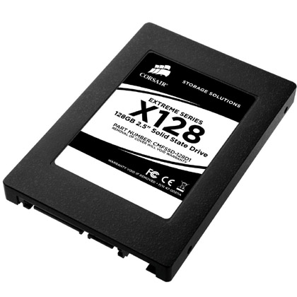
Figure 11-7 A solid-state drive (photo courtesy of Corsair)
Solid-state devices use current flow and negative/positive electron charges to achieve their magic. Although Mr. Spock may find the physics of how this technology actually works “fascinating,” it’s more important for you to know the following points regarding solid-state drives, devices, and technology.
NOTE With solid-state drives coming into more regular use, you see the initials HDD used more frequently than in previous years to refer to the traditional, platter-based hard drives. Thus we have two drive technologies: SSDs and HDDs.
• Solid-state technology is commonly used in desktop and laptop hard drives, memory cards, cameras, USB thumb drives, and other handheld devices.
SSD form factors are typically 1.8-inch, 2.5-inch, or 3.5-inch.
• SSDs can be PATA, SATA, eSATA, SCSI, or USB for desktop systems. Some portable computers have mini-PCI Express versions. You can also purchase SSD cards built onto PCIe cards (which you would connect to your PC like any other expansion card).
• SSDs that use SDRAM cache are volatile and lose data when powered off. Others that use nonvolatile flash memory such as NAND retain data when power is turned off or disconnected. (See Chapter 13 for the scoop on flash memory technology.)
• SSDs are more expensive than traditional HDDs. Less expensive SSDs typically implement less reliable multi-level cell (MLC) memory technology in place of the more efficient single-level cell (SLC) technology to cut costs.
 EXAM TIP The term IDE (integrated drive electronics) refers to any hard drive with a built-in controller. All hard drives are technically IDE drives, although we only use the term IDE when discussing ATA drives.
Over the years, many interfaces existed for hard drives, with such names as ST-506 and ESDI. Don’t worry about what these abbreviations stood for; neither the CompTIA A+ certification exams nor the computer world at large have an interest in these prehistoric interfaces. Starting around 1990, an interface called advanced technology attachment (ATA) appeared that now virtually monopolizes the hard drive market. ATA hard drives are often referred to as integrated drive electronics (IDE) drives. Only one other type of interface, the moderately popular small computer system interface (SCSI), has any relevance for hard drives.
ATA drives come in two basic flavors. The older parallel ATA (PATA) drives send data in parallel, on a 40- or 80-wire data cable. PATA drives dominated the industry for more than a decade but have been mostly replaced by serial ATA (SATA) drives that send data in serial, using only one wire for data transfers. The leap from PATA to SATA is only one of a large number of changes that have taken place with ATA. To appreciate these changes, we’ll run through the many ATA standards that have appeared over the years.
NOTE A quick trip to any major computer store will reveal a thriving trade in external hard drives. You used to be able to find external drives that connected to the slow parallel port, but external drives today connect to a FireWire, USB, or eSATA port. All three interfaces offer high data transfer rates and hot-swap capability, making them ideal for transporting huge files such as digital video clips. Regardless of the external interface, however, you’ll find an ordinary PATA or SATA drive inside the external enclosure (the name used to describe the casing of external hard drives).
When IBM unveiled the 80286-powered IBM PC AT in the early 1980s, it introduced the first PC to include BIOS support for hard drives. This BIOS supported up to two physical drives, and each drive could be up to 504 MB—far larger than the 5-MB and 10-MB drives of the time. Although having built-in support for hard drives certainly improved the power of the PC, installing, configuring, and troubleshooting hard drives could at best be called difficult at that time.
To address these problems, Western Digital and Compaq developed a new hard drive interface and placed this specification before the American National Standards Institute (ANSI) committees, which in turn put out the AT Attachment (ATA) interface in March of 1989. The ATA interface specified a cable and a built-in controller on the drive itself. Most importantly, the ATA standard used the existing AT BIOS on a PC, which meant that you didn’t have to replace the old system BIOS to make the drive work—a very important consideration for compatibility but one that would later haunt ATA drives. The official name for the standard, ATA, never made it into the common vernacular until recently, and then only as PATA to distinguish it from SATA drives.
The first ATA drives connected to the computer with a 40-pin ribbon cable that plugged into the drive and into a hard drive controller. The cable has a colored stripe down one side that denotes pin 1 and should connect to the drive’s pin 1 and to the controller’s pin 1. Figure 11-8 shows the business end of an early ATA drive, with the connectors for the ribbon cable and the power cable.
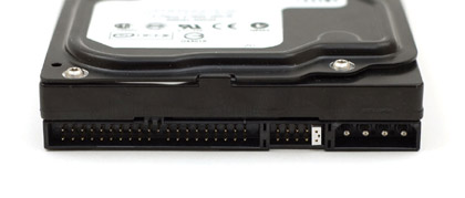
Figure 11-8 Back of IDE drive showing 40-pin connector (left), jumpers (center), and power connector (right)
The controller is the support circuitry that acts as the intermediary between the hard drive and the external data bus. Electronically, the setup looks like Figure 11-9.
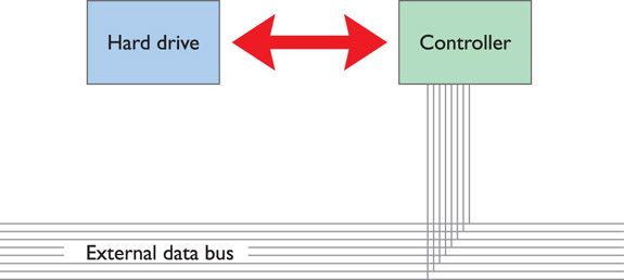
Figure 11-9 Relation of drive, controller, and bus
Wait a minute! If ATA drives are IDE (see the earlier Exam Tip), they already have a built-in controller. Why do they then have to plug into a controller on the motherboard? Well, this is a great example of a term that’s not used properly, but everyone (including the motherboard and hard drive makers) uses it this way. What we call the ATA controller is really no more than an interface providing a connection to the rest of the PC system. When your BIOS talks to the hard drive, it actually talks to the onboard circuitry on the drive, not the connection on the motherboard. But, even though the real controller resides on the hard drive, the 40-pin connection on the motherboard is called the controller. We have a lot of misnomers to live with in the ATA world.
The ATA-1 standard defined that no more than two drives attach to a single IDE connector on a single ribbon cable. Because up to two drives can attach to one connector via a single cable, you need to be able to identify each drive on the cable. The ATA standard identifies the two drives as “master” and “slave.” You set one drive as master and one as slave by using tiny jumpers on the drives (see Figure 11-10).
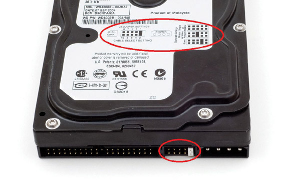
Figure 11-10 A typical hard drive with directions (top) for setting a jumper (bottom)
The controllers are on the motherboard and manifest themselves as two 40-pin male ports, as shown in Figure 11-11.
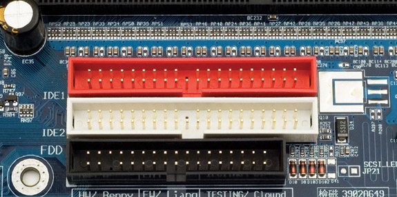
Figure 11-11 IDE interfaces on a motherboard
NOTE The ANSI subcommittee directly responsible for the ATA standard is called Technical Committee T13. If you want to know what’s happening with ATA, check out the T13 Web site: www.t13.org.
If you’re making a hard drive standard, you must define both the method and the speed at which the data’s going to move.
ATA-1 defined two methods, the first using programmed I/O (PIO) addressing and the second using direct memory access (DMA) mode.
PIO is nothing more than the traditional I/O addressing scheme, where the CPU talks directly to the hard drive via the BIOS to send and receive data. Three different PIO speeds called PIO modes were initially adopted:
• PIO mode 0: 3.3 MBps (megabytes per second)
• PIO mode 1: 5.2 MBps
• PIO mode 2: 8.3 MBps
DMA modes defined a method to enable the hard drives to talk to RAM directly, using old-style DMA commands. (The ATA folks called this single-word DMA.) This old-style DMA was slow, and the resulting three ATA single-word DMA modes were also slow:
• Single-word DMA mode 0: 2.1 MBps
• Single-word DMA mode 1: 4.2 MBps
• Single-word DMA mode 2: 8.3 MBps
When a computer booted up, the BIOS queried the hard drive to see what modes it could use and then automatically adjusted to the fastest possible mode.
In 1990, the industry adopted a series of improvements to the ATA standard called ATA-2. Many people called these new features Enhanced IDE (EIDE). EIDE was really no more than a marketing term invented by Western Digital, but it caught on in common vernacular and is still used today, although its use is fading. Regular IDE drives quickly disappeared, and by 1995, EIDE drives dominated the PC world. Figure 11-12 shows a typical EIDE drive.

Figure 11-12 EIDE drive
ATA-2 was the most important ATA standard, as it included powerful new features such as higher capacities, support for non-hard drive storage devices, support for two more ATA devices for a maximum of four, and substantially improved throughput.
NOTE The terms ATA, IDE, and EIDE are used interchangeably.
IBM created the AT BIOS to support hard drives many years before IDE drives were invented, and every system had that BIOS. The developers of IDE made certain that the new drives would run from the same AT BIOS command set. With this capability, you could use the same CMOS and BIOS routines to talk to a much more advanced drive. Your motherboard or hard drive controller wouldn’t become instantly obsolete when you installed a new hard drive.
Unfortunately, the BIOS routines for the original AT command set allowed a hard drive size of only up to 528 million bytes (or 504 MB—remember that a mega = 1,048,576, not 1,000,000). A drive could have no more than 1024 cylinders, 16 heads, and 63 sectors/track:
1024 cylinders × 16 heads × 63 sectors/track × 512 bytes/sector = 504 MB
For years, this was not a problem. But when hard drives began to approach the 504-MB barrier, it became clear that there needed to be a way of getting past 504 MB. The ATA-2 standard defined a way to get past this limit with logical block addressing (LBA). With LBA, the hard drive lies to the computer about its geometry through an advanced type of sector translation. Let’s take a moment to understand sector translation, and then come back to LBA.
Long before hard drives approached the 504-MB limit, the limits of 1024 cylinders, 16 heads, and 63 sectors/track gave hard drive makers fits. The big problem was the heads. Remember that every two heads means another platter, another physical disk that you have to squeeze into a hard drive. If you wanted a hard drive with the maximum number of 16 heads, you would need a hard drive with eight physical platters inside the drive. Nobody wanted that many platters: it made the drives too tall, it took more power to spin up the drive, and that many parts cost too much money (see Figure 11-13).
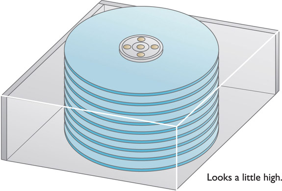
Figure 11-13 Too many heads
Manufacturers could readily produce a hard drive that had fewer heads and more cylinders, but the stupid 1024/16/63 limit got in the way. Plus, the traditional sector arrangement wasted a lot of useful space. Sectors toward the inside of the drive, for example, are much shorter than the sectors on the outside. The sectors on the outside don’t need to be that long, but with the traditional geometry setup, hard drive makers had no choice. They could make a hard drive store a lot more information, however, if they could make hard drives with more sectors/track on the outside tracks (see Figure 11-14).
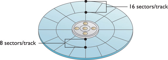
Figure 11-14 Multiple sectors/track
The ATA specification was designed to have two geometries. The physical geometry defined the real layout of the CHS inside the drive. The logical geometry described what the drive told the CMOS. In other words, the IDE drive “lied” to the CMOS, thus sidestepping the artificial limits of the BIOS. When data was being transferred to and from the drive, the onboard circuitry of the drive translated the logical geometry into the physical geometry. This function was, and still is, called sector translation.
Let’s look at a couple of hypothetical examples in action. First, pretend that Seagate came out with a new, cheap, fast hard drive called the ST108. To get the ST108 drive fast and cheap, however, Seagate had to use a rather strange geometry, shown in Table 11-1.
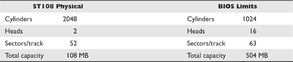
Table 11-1 Seagate’s ST108 Drive Geometry
NOTE Hard drive makers talk about hard drive capacities in millions and billions of bytes, not megabytes and gigabytes.
Notice that the cylinder number is greater than 1024. To overcome this problem, the IDE drive performs a sector translation that reports a geometry to the BIOS that is totally different from the true geometry of the drive. Table 11-2 shows the physical geometry and the “logical” geometry of our mythical ST108 drive. Notice that the logical geometry is now within the acceptable parameters of the BIOS limitations. Sector translation never changes the capacity of the drive; it changes only the geometry to stay within the BIOS limits.
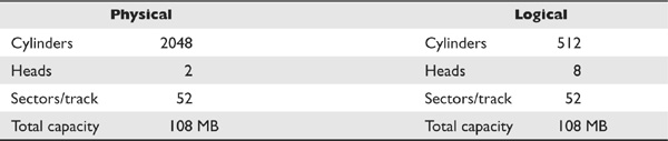
Table 11-2 Physical and Logical Geometries of the ST108 Drive
Now let’s watch how the advanced sector translation of LBA provides support for hard drives greater than 504 MB. Let’s use an old drive, the Western Digital WD2160, a 2.1-GB hard drive, as an example. This drive is no longer in production, but its smaller CHS values make understanding LBA easier. Table 11-3 lists its physical and logical geometries.
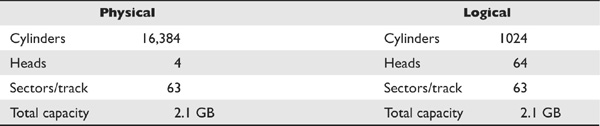
Table 11-3 Western Digital WD2160’s Physical and Logical Geometries
Note that, even with sector translation, the number of heads is greater than the allowed 16. So here’s where the magic of LBA comes in. When the computer boots up, the BIOS asks the drives if they can perform LBA. If they say yes, the BIOS and the drive work together to change the way they talk to each other. They can do this without conflicting with the original AT BIOS commands by taking advantage of unused commands to use up to 256 heads. LBA enables support for a maximum of 1024 × 256 × 63 × 512 bytes = 8.4-GB hard drives. Back in 1990, 8.4 GB was hundreds of times larger than the drives used at the time. Don’t worry, later ATA standards will get the BIOS up to today’s huge drives.
ATA-2 added an extension to the ATA specification, called advanced technology attachment packet interface (ATAPI), that enabled non-hard drive devices such as CD-ROM drives and tape backups to connect to the PC via the ATA controllers. ATAPI drives have the same 40-pin interface and master/slave jumpers as ATA hard drives. Figure 11-15 shows an ATAPI CD-RW drive attached to a motherboard. The key difference between hard drives and every other type of drive that attaches to the ATA controller is in how the drives get BIOS support. Hard drives get it through the system BIOS, whereas non–hard drives require the operating system to load a software driver.

Figure 11-15 ATAPI CD-RW drive attached to a motherboard via a standard 40-pin ribbon cable
NOTE With the introduction of ATAPI, the ATA standards are often referred to as ATA/ATAPI instead of just ATA.
ATA-2 added support for a second controller, raising the total number of supported drives from two to four. Each of the two controllers is equal in power and capability. Figure 11-16 is a close-up of a typical motherboard, showing the primary controller marked as PRI_IDE and the secondary marked as SEC_IDE.
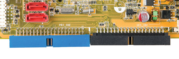
Figure 11-16 Primary and secondary controllers labeled on a motherboard
ATA-2 defined two new PIO modes and a new type of DMA called multi-word DMA that was a substantial improvement over the old DMA. Technically, multi-word DMA was still the old-style DMA, but it worked in a much more efficient manner, so it was much faster.
• PIO mode 4: 16.6 MBps
• Multi-word DMA mode 0: 4.2 MBps
• Multi-word DMA mode 1: 13.3 MBps
• Multi-word DMA mode 2: 16.6 MBps
ATA-3 came on quickly after ATA-2 and added one new feature called Self-Monitoring, Analysis, and Reporting Technology (S.M.A.R.T.), one of the few PC acronyms that requires the use of periods after each letter. S.M.A.R.T. helps predict when a hard drive is going to fail by monitoring the hard drive’s mechanical components.
S.M.A.R.T. is a great idea and is popular in specialized server systems, but it’s complex, imperfect, and hard to understand. As a result, only a few utilities can read the S.M.A.R.T. data on your hard drive. Your best sources are the hard drive manufacturers. Every hard drive maker has a free diagnostic tool (which usually works only for their drives) that will do a S.M.A.R.T. check along with other tests. Figure 11-17 shows Western Digital’s Data Lifeguard Tools in action. Note that it says only whether the drive has passed or not. Figure 11-18 shows some S.M.A.R.T. information.
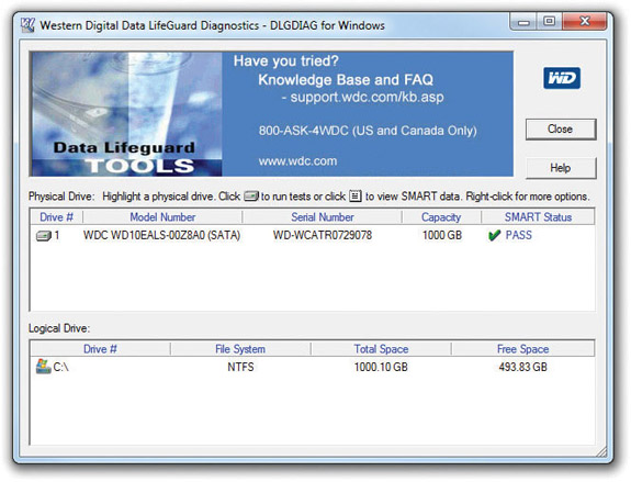
Figure 11-17 Data Lifeguard Tools
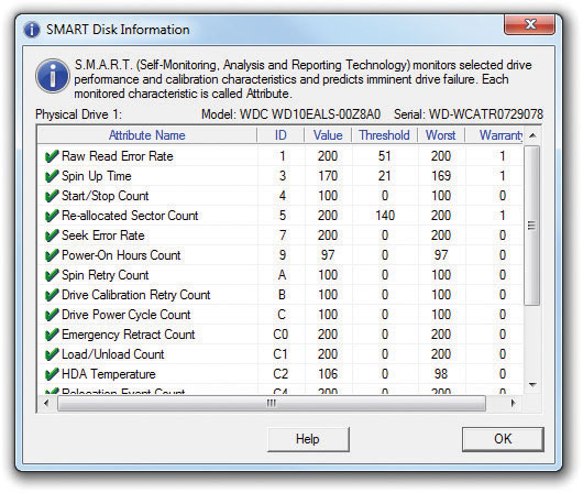
Figure 11-18 S.M.A.R.T. information
Although you can see the actual S.M.A.R.T. data, it’s generally useless or indecipherable. Your best choice is to trust the manufacturer’s opinion and run the software provided.
Anyone who has opened a big database file on a hard drive appreciates that a faster hard drive is better. ATA-4 introduced a new DMA mode called Ultra DMA that is now the primary way a hard drive communicates with a PC. Ultra DMA uses DMA bus mastering to achieve far faster speeds than were possible with PIO or old-style DMA. ATA-4 defined three Ultra DMA modes:
• Ultra DMA mode 0: 16.7 MBps
• Ultra DMA mode 1: 25.0 MBps
• Ultra DMA mode 2: 33.3 MBps
NOTE Ultra DMA mode 2, the most popular of the ATA-4 DMA modes, is also called ATA/33.
Here’s an interesting factoid for you: The original ATA-1 standard allowed for hard drives up to 137 GB. It wasn’t the ATA standard that caused the 504-MB size limit; the standard used the old AT BIOS, and the BIOS, not the ATA standard, could support only 504 MB. LBA was a work-around that told the hard drive to lie to the BIOS to get it up to 8.4 GB. But eventually hard drives started edging close to the LBA limit and something had to be done. The T13 folks said, “This isn’t our problem. It’s the ancient BIOS problem. You BIOS makers need to fix the BIOS.” And they did.
In 1994, Phoenix Technologies (the BIOS manufacturer) came up with a new set of BIOS commands called Interrupt 13 (INT13) extensions. INT13 extensions broke the 8.4-GB barrier by completely ignoring the CHS values and instead feeding the LBA a stream of addressable sectors. A system with INT13 extensions can handle drives up to 137 GB. The entire PC industry quickly adopted INT13 extensions, and every system made since 2000-2001 supports INT13 extensions.
Ultra DMA was such a huge hit that the ATA folks adopted two faster Ultra DMA modes with ATA-5:
• Ultra DMA mode 3: 44.4 MBps
• Ultra DMA mode 4: 66.6 MBps
Ultra DMA mode 4 ran so quickly that the ATA-5 standard defined a new type of ribbon cable that could handle the higher speeds. This 80-wire cable still has 40 pins on the connectors, but it also includes another 40 wires in the cable that act as grounds to improve the cable’s capability to handle high-speed signals. The 80-wire cable, just like the 40-pin ribbon cable, has a colored stripe down one side to give you proper orientation for pin 1 on the controller and the hard drive. Previous versions of ATA didn’t define where the various drives were plugged into the ribbon cable, but ATA-5 defined exactly where the controller, master, and slave drives connected, even defining colors to identify them. Take a look at the ATA/66 cable in Figure 11-19. The connector on the left is colored blue—and you must use that connector to plug into the controller. The connector in the middle is gray—that’s for the slave drive. The connector on the right is black—that’s for the master drive. Any ATA/66 controller connections are colored blue to let you know it is an ATA/66 controller.
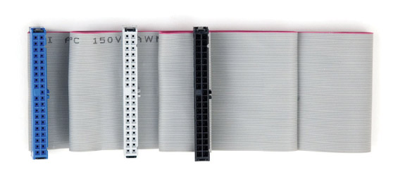
Figure 11-19 ATA/66 cable
ATA/66 is backward compatible, so you may safely plug an earlier drive into an ATA/66 cable and controller. If you plug an ATA/66 drive into an older controller, it will work—just not in ATA/66 mode. The only risky action is to use an ATA/66 controller and hard drive with a non-ATA/66 cable. Doing so will almost certainly cause nasty data losses!
Hard drive size exploded in the early 21st century, and the seemingly impossible-to-fill 137-GB limit created by INT13 extensions became a barrier earlier than most people had anticipated. When drives started hitting the 120-GB mark, the T13 committee adopted an industry proposal pushed by Maxtor (a major hard drive maker) called Big Drive that increased the limit to more than 144 petabytes (approximately 144,000,000 GB). Thankfully, T13 also gave the new standard a less-silly name, calling it ATA/ATAPI-6 or simply ATA-6. Big Drive was basically just a 48-bit LBA, supplanting the older 24-bit addressing of LBA and INT13 extensions. Plus, the standard defined an enhanced block mode, enabling drives to transfer up to 65,536 sectors in one chunk, up from the measly 256 sectors of lesser drive technologies.
ATA-6 also introduced Ultra DMA mode 5, kicking the data transfer rate up to 100 MBps. Ultra DMA mode 5 is more commonly referred to as ATA/100 and requires the same 80-wire cable as ATA/66.
NOTE Ultra DMA mode 4, the most popular of the ATA-5 DMA modes, is also called ATA/66.
ATA-7 brought two new innovations to the ATA world: one evolutionary and the other revolutionary. The evolutionary innovation came with the last of the parallel ATA Ultra DMA modes; the revolutionary was a new form of ATA called serial ATA (SATA).
ATA-7 introduced the fastest and probably least adopted of all of the ATA speeds, Ultra DMA mode 6 (ATA/133). Even though it runs at a speed of 133 MBps, the fact that it came out with SATA kept many hard drive manufacturers away. ATA/133 uses the same cables as Ultra DMA 66 and 100.
While you won’t find many ATA/133 hard drives, you will find plenty of ATA/133 controllers. There’s a trend in the industry to color the controller connections on the hard drive red, although this is not part of the ATA-7 standard.
The real story of ATA-7 is SATA. For all its longevity as the mass storage interface of choice for the PC, parallel ATA has problems. First, the flat ribbon cables impede airflow and can be a pain to insert properly. Second, the cables have a limited length, only 18 inches. Third, you can’t hot-swap PATA drives. You have to shut down completely before installing or replacing a drive. Finally, the technology has simply reached the limits of what it can do in terms of throughput.
Serial ATA addresses these issues. SATA creates a point-to-point connection between the SATA device—hard disk, CD-ROM, CD-RW, DVD-ROM, DVD-RW, BD-R, BD-RE, and so on—and the SATA controller, the host bus adapter (HBA). At a glance, SATA devices look identical to standard PATA devices. Take a closer look at the cable and power connectors, however, and you’ll see significant differences (see Figure 11-20).
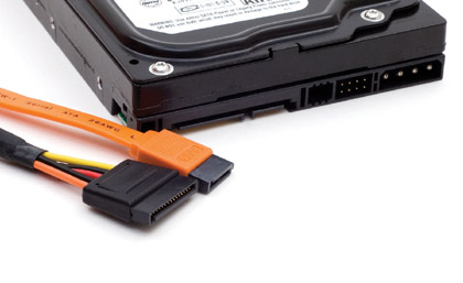
Figure 11-20 SATA hard disk power (left) and data (right) cables
Because SATA devices send data serially instead of in parallel, the SATA interface needs far fewer physical wires—seven instead of the eighty wires that is typical of PATA—resulting in much thinner cabling. This might not seem significant, but the benefit is that thinner cabling means better cable control and better airflow through the PC case, resulting in better cooling.
Further, the maximum SATA-device cable length is more than twice that of an IDE cable—about 40 inches (1 meter) instead of 18 inches. Again, this might not seem like a big deal unless you’ve struggled to connect a PATA hard disk installed into the top bay of a full-tower case to an IDE connector located all the way at the bottom of the motherboard.
SATA does away with the entire master/slave concept. Each drive connects to one port, so no more daisy-chaining drives. Further, there’s no maximum number of drives—many motherboards are now available that support up to eight SATA drives. Want more? Snap in a SATA HBA and load ’em up!
NOTE Number-savvy readers might have noticed a discrepancy between the names and throughput of SATA drives. After all, SATA 1.0’s 1.5-Gbps throughput translates to 192 MBps, a lot higher than the advertised speed of a “mere” 150 MBps. The encoding scheme used on SATA drives takes about 20 percent of the overhead for the drive, leaving 80 percent for pure bandwidth. SATA 2.0’s 3-Gbps drive created all kinds of problems, because the committee working on the specifications was called the SATA II committee, and marketers picked up on the SATA II name. As a result, you’ll find many hard drives labeled “SATA II” rather than 3 Gbps. The SATA committee now goes by the name SATA-IO.
The big news, however, is in data throughput. As the name implies, SATA devices transfer data in serial bursts instead of parallel, as PATA devices do. Typically, you might not think of serial devices as being faster than parallel, but in this case, a SATA device’s single stream of data moves much faster than the multiple streams of data coming from a parallel IDE device—theoretically, up to 30 times faster. SATA drives come in three common varieties: 1.5 Gbps, 3 Gbps, and 6 Gbps, which have a maximum throughput of 150 MBps, 300 MBps, and 600 MBps, respectively.
EXAM TIP Each SATA variety is named for the revision to the SATA specification that introduced it:
• SATA 1.0: 1.5 Gbps
• SATA 2.0: 3 Gbps
• SATA 3.0: 6 Gbps
SATA is backward compatible with current PATA standards and enables you to install a parallel ATA device, including a hard drive, optical drive, and other devices, to a serial ATA controller by using a SATA bridge. A SATA bridge manifests as a tiny card that you plug directly into the 40-pin connector on a PATA drive. As you can see in Figure 11-21, the controller chip on the bridge requires separate power; you plug a Molex connector into the PATA drive as normal. When you boot the system, the PATA drive shows up to the system as a SATA drive.

Figure 11-21 SATA bridge
SATA’s ease of use has made it the choice for desktop system storage, and its success is already showing in the fact that more than 90 percent of all hard drives sold today are SATA drives.
Windows Vista and later operating systems support the Advanced Host Controller Interface (AHCI), a more efficient way to work with SATA HBAs. Using AHCI unlocks some of the advanced features of SATA, such as hot-swapping and native command queuing.
When you plug in a SATA drive to a running Windows computer that does not have AHCI enabled, the drive doesn’t appear automatically. In Windows XP/Vista, you need to go to the Control Panel and run the Add New Hardware to make the drive appear, and in Windows 7, you need to run hdwwiz.exe from the Start menu Search bar. With AHCI, the drive should appear in My Computer/Computer immediately, just what you’d expect from a hot-swappable device.
Native command queuing (NCQ) is a disk-optimization feature for SATA drives. It enables faster read and write speeds.
AHCI is implemented at the CMOS level (see “BIOS Support: Configuring CMOS and Installing Drivers,” later in this chapter) and generally needs to be enabled before you install the operating system. Enabling it after installation will cause Windows Vista and 7 to Blue Screen. How nice.
 TIP If you want to enable AHCI but you’ve already installed Windows Vista or Windows 7, don’t worry! Microsoft has developed a procedure (http://support. microsoft.com/kb/922976) that will have you enjoying all that AHCI fun in no time. Before you jump in, note that this procedure requires you to edit your Registry, so remember to always make a backup before you start editing.
External SATA (eSATA) extends the SATA bus to external devices, as the name would imply. The eSATA drives use connectors similar to internal SATA, but they’re keyed differently so you can’t mistake one for the other. Figure 11-22 shows eSATA connectors on the back of a motherboard.

Figure 11-22 eSATA connectors
External SATA uses shielded cable lengths up to 2 meters outside the PC and is hot-swappable. The beauty of eSATA is that it extends the SATA bus at full speed, which tops out at a theoretical 6 Gbps, whereas the fastest USB connection (USB 3.0, also called SuperSpeed USB) maxes out at 5 Gbps. It’s not that big of a speed gap, especially when you consider that neither connection type fully utilizes its bandwidth yet, but even in real-world tests, eSATA still holds its own.
If a desktop system doesn’t have an eSATA external connector, or if you need more external SATA devices, you can install an eSATA HBA PCIe card or eSATA internal-to-external slot plate. You can similarly upgrade laptop systems to support external SATA devices by inserting an eSATA ExpressCard (see Figure 11-23). There are also USB-to-eSATA adapter plugs. Install eSATA PCIe, PC Card, or ExpressCard following the same rules and precautions for installing any expansion device.
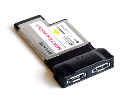
Figure 11-23 eSATA ExpressCard
NOTE In addition to eSATA ports, you’ll also run into eSATAp ports on some laptops. This port physically combines a powered USB connection with a speedy eSATA connection; you can connect a USB, eSATA, or special eSATAp cable into the port. eSATAp enables you to connect an internal drive (HDD, SSD, or optical drive) to your laptop without an enclosure, using a single cable to power it and send/receive data.
Many specialized server machines and enthusiasts’ systems use the small computer system interface (SCSI) technologies for various pieces of core hardware and peripherals, from hard drives to printers to high-end tape-backup machines. SCSI, pronounced “scuzzy,” is different from ATA in that SCSI devices connect together in a string of devices called a chain. Each device in the chain gets a SCSI ID to distinguish it from other devices on the chain. Last, the ends of a SCSI chain must be terminated. Let’s dive into SCSI now, and see how SCSI chains, SCSI IDs, and termination all work.
SCSI is an old technology dating from the late 1970s, but it has been updated continually. SCSI is faster than ATA (though the gap is closing fast), and until SATA arrived, SCSI was the only good choice for anyone using RAID (see the “RAID” section a little later). SCSI is arguably fading away, but it deserves some mention.
SCSI manifests itself through a SCSI chain, a series of SCSI devices working together through a host adapter. The host adapter provides the interface between the SCSI chain and the PC. Figure 11-24 shows a typical SCSI PCI host adapter. Many techs refer to the host adapter as the SCSI controller, so you should be comfortable with both terms.
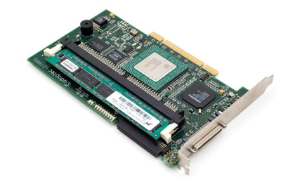
Figure 11-24 SCSI host adapter
All SCSI devices can be divided into two groups: internal and external. Internal SCSI devices are attached inside the PC and connect to the host adapter through the latter’s internal connector. Figure 11-25 shows an internal SCSI device, in this case a CD-ROM drive. External devices hook to the external connector of the host adapter. Figure 11-26 is an example of an external SCSI device.
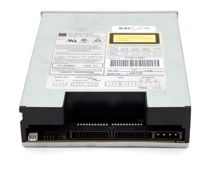
Figure 11-25 Internal SCSI CD-ROM
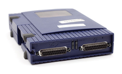
Figure 11-26 Back of external SCSI device
Internal SCSI devices connect to the host adapter with a 68-pin ribbon cable (see Figure 11-27). This flat, flexible cable functions precisely like a PATA cable. Many external devices connect to the host adapter with a 50-pin high-density (HD) connector. Figure 11-28 shows a host adapter external port. Higher-end SCSI devices use a 68-pin HD connector.
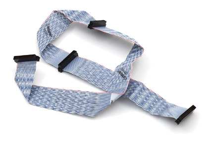
Figure 11-27 Typical 68-pin ribbon cable
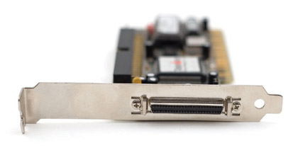
Figure 11-28 50-pin HD port on SCSI host adapter
EXAM TIP Some early versions of SCSI used a 25-pin connector. This connector was much more popular on Apple devices, though it did see use on PCs with the old SCSI Zip drives. While the connector is now obsolete, you need to know about it for the CompTIA A+ exams.
Multiple internal devices can be connected simply by using a cable with enough connectors (see Figure 11-29). The 68-pin ribbon cable shown in Figure 11-27, for example, can support up to four SCSI devices, including the host adapter.
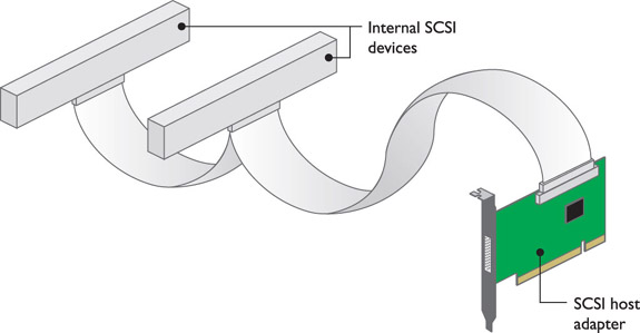
Figure 11-29 Internal SCSI chain with two devices
Assuming the SCSI host adapter has a standard external port (some controllers don’t have external connections at all), plugging in an external SCSI device is as simple as running a cable from device to controller. The external SCSI connectors are D-shaped so you can’t plug them in backward. As an added bonus, some external SCSI devices have two ports, one to connect to the host adapter and a second to connect to another SCSI device. The process of connecting a device directly to another device is called daisy-chaining. You can daisy-chain as many as 15 devices to one host adapter. SCSI chains can be internal, external, or both (see Figure 11-30).
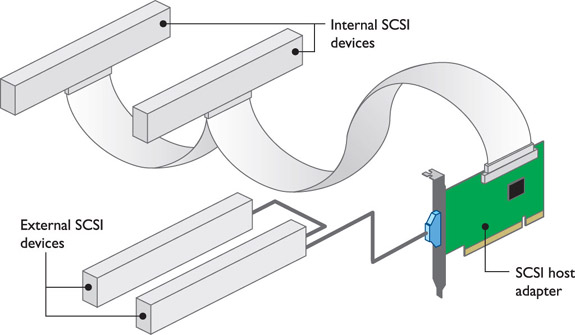
Figure 11-30 Internal and external devices on one SCSI chain
If you’re going to connect a number of devices on the same SCSI chain, you must provide some way for the host adapter to tell one device from another. To differentiate devices, SCSI uses a unique identifier called the SCSI ID. The SCSI ID number can range from 0 to 15. SCSI IDs are similar to many other PC hardware settings in that a SCSI device can theoretically have any SCSI ID as long as that ID is not already taken by another device connected to the same host adapter.
Some conventions should be followed when setting SCSI IDs. Typically, most people set the host adapter to 7 or 15, but you can change this setting. Note that there is no order for the use of SCSI IDs. It does not matter which device gets which number, and you can skip numbers. Restrictions on IDs apply only within a single chain. Two devices can have the same ID, in other words, as long as they are on different chains (see Figure 11-31).
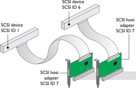
Figure 11-31 IDs don’t conflict between separate SCSI chains.
Every SCSI device has some method of setting its SCSI ID. The trick is to figure out how as you’re holding the device in your hand. A SCSI device may use jumpers, dip switches, or even tiny dials; every new SCSI device is a new adventure as you try to determine how to set its SCSI ID.
NOTE Old SCSI equipment allowed SCSI IDs from 0 to 7 only.
Whenever you send a signal down a wire, some of that signal reflects back up the wire, creating an echo and causing electronic chaos. SCSI chains use termination to prevent this problem. Termination simply means putting something on the ends of the wire to prevent this echo. Terminators are usually pull-down resistors and can manifest themselves in many different ways. Most of the devices within a PC have the appropriate termination built in. On other devices, including SCSI chains and some network cables, you have to set termination during installation.
The rule with SCSI is that you must terminate only the ends of the SCSI chain. You have to terminate the ends of the cable, which usually means that you need to terminate the two devices at the ends of the cable. Do not terminate devices that are not on the ends of the cable. Figure 11-32 shows some examples of where to terminate SCSI devices.

Figure 11-32 Location of the terminated devices
Because any SCSI device might be on the end of a chain, most manufacturers build SCSI devices that can self-terminate. Some devices can detect that they are on the end of the SCSI chain and automatically terminate themselves. Most devices, however, require you to set a jumper or switch to enable termination (see Figure 11-33).
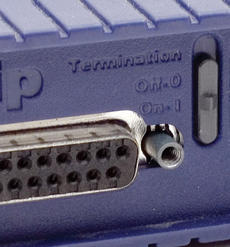
Figure 11-33 Setting termination
Ask experienced techs “What is the most expensive part of a PC?” and they’ll all answer in the same way: “It’s the data.” You can replace any single part of your PC for a few hundred dollars at most, but if you lose critical data—well, let’s just say I know of two small companies that went out of business because they lost a hard drive full of data.
Data is king; data is your PC’s raison d’être. Losing data is a bad thing, so you need some method to prevent data loss. Of course, you can do backups, but if a hard drive dies, you have to shut down the computer, reinstall a new hard drive, reinstall the operating system, and then restore the backup. There’s nothing wrong with this as long as you can afford the time and cost of shutting down the system.
A better solution, though, would save your data if a hard drive died and enable you to continue working throughout the process. This is possible if you stop relying on a single hard drive and instead use two or more drives to store your data. Sounds good, but how do you do this? Well, first of all, you could install some fancy hard drive controller that reads and writes data to two hard drives simultaneously (see Figure 11-34). The data on each drive would always be identical. One drive would be the primary drive and the other drive, called the mirror drive, would not be used unless the primary drive failed. This process of reading and writing data at the same time to two drives is called disk mirroring.
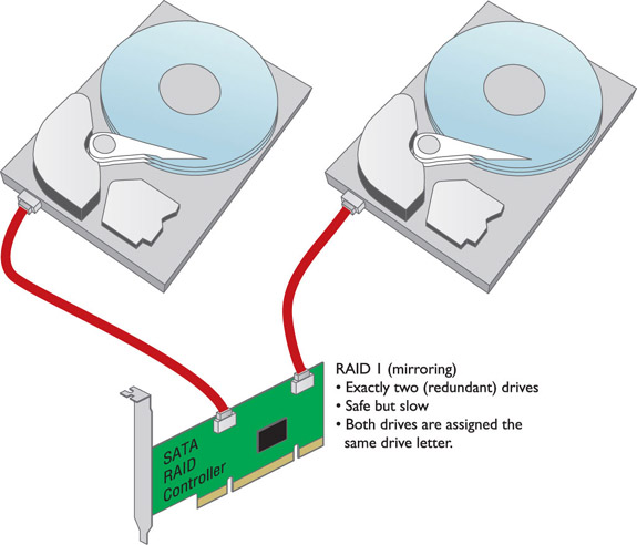
Figure 11-34 Mirrored drives
If you really want to make data safe, you can use a separate controller for each drive. With two drives, each on a separate controller, the system will continue to operate even if the primary drive’s controller stops working. This super-drive mirroring technique is called disk duplexing (see Figure 11-35). Disk duplexing is also much faster than disk mirroring because one controller does not write each piece of data twice.
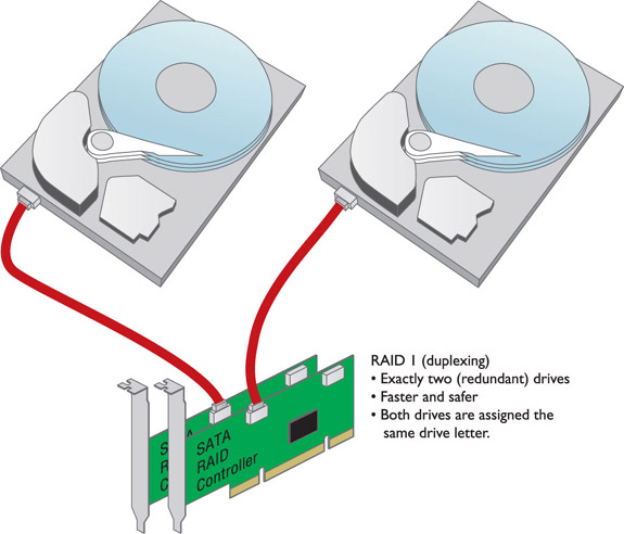
Figure 11-35 Duplexing drives
Even though duplexing is faster than mirroring, they both are slower than the classic one-drive, one-controller setup. You can use multiple drives to increase your hard drive access speed. Disk striping (without parity) means spreading the data among multiple (at least two) drives. Disk striping by itself provides no redundancy. If you save a small Microsoft Word file, for example, the file is split into multiple pieces; half of the pieces go on one drive and half on the other (see Figure 11-36).
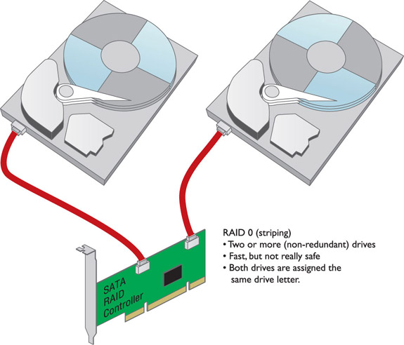
Figure 11-36 Disk striping
The one and only advantage of disk striping is speed—it is a fast way to read and write to hard drives. But if either drive fails, all data is lost. You should not do disk striping—unless you’re willing to increase the risk of losing data to increase the speed at which your hard drives save and restore data.
Disk striping with parity, in contrast, protects data by adding extra information, called parity data, that can be used to rebuild data if one of the drives fails. Disk striping with parity requires at least three drives, but it is common to use more than three. Disk striping with parity combines the best of disk mirroring and plain disk striping. It protects data and is quite fast. The majority of network servers use a type of disk striping with parity.
A couple of sharp guys in Berkeley back in the 1980s organized the many techniques for using multiple drives for data protection and increasing speeds as the redundant array of independent (or inexpensive) disks (RAID). They outlined seven levels of RAID, numbered 0 through 6:
• RAID 0—Disk Striping Disk striping requires at least two drives. It does not provide redundancy to data. If any one drive fails, all data is lost.
• RAID 1—Disk Mirroring/Duplexing RAID 1 arrays require at least two hard drives, although they also work with any even number of drives. RAID 1 is the ultimate in safety, but you lose storage space because the data is duplicated; you need two 100-GB drives to store 100 GB of data.
• RAID 2—Disk Striping with Multiple Parity Drives RAID 2 was a weird RAID idea that never saw practical use. Ignore it.
• RAID 3 and 4—Disk Striping with Dedicated Parity RAID 3 and 4 combined dedicated data drives with dedicated parity drives. The differences between the two are trivial. Unlike RAID 2, these versions did see some use in the real world but were quickly replaced by RAID 5.
• RAID 5—Disk Striping with Distributed Parity Instead of dedicated data and parity drives, RAID 5 distributes data and parity information evenly across all drives. This is the fastest way to provide data redundancy. RAID 5 is by far the most common RAID implementation and requires at least three drives. RAID 5 arrays effectively use one drive’s worth of space for parity. If, for example, you have three 200-GB drives, your total storage capacity is 400 GB. If you have four 200-GB drives, your total capacity is 600 GB.
• RAID 6—Disk Striping with Extra Parity If you lose a hard drive in a RAID 5 array, your data is at great risk until you replace the bad hard drive and rebuild the array. RAID 6 is RAID 5 with extra parity information. RAID 6 needs at least five drives, but in exchange you can lose up to two drives at the same time. RAID 6 is gaining in popularity for those willing to use larger arrays.
NOTE An array in the context of RAID refers to a collection of two or more hard drives. No tech worth her salt says such things as “We’re implementing disk striping with parity.” Use the RAID level. Say, “We’re implementing RAID 5.” It’s more accurate and very impressive to the folks in the accounting department!
After these first RAID levels were defined, some manufacturers came up with ways to combine different RAIDs. For example, what if you took two pairs of striped drives and mirrored the pairs? You would get what is called RAID 0+1. Or what if (read this carefully now) you took two pairs of mirrored drives and striped the pairs? You then get what we call RAID 1+0 or what is often called RAID 10. Combinations of different types of single RAID are called multiple RAID or nested RAID solutions.
NOTE There is actually a term for a storage system composed of multiple independent disks rather than disks organized by using RAID: JBOD, which stands for just a bunch of disks (or drives).
RAID levels describe different methods of providing data redundancy or enhancing the speed of data throughput to and from groups of hard drives. They do not say how to implement these methods. Literally thousands of methods can be used to set up RAID. The method you use depends largely on the level of RAID you desire, the operating system you use, and the thickness of your wallet.
The obvious starting place for RAID is to connect at least two hard drives in some fashion to create a RAID array. For many years, if you wanted to do RAID beyond RAID 0 and RAID 1, the only technology you could use was good-old SCSI. SCSI’s chaining of multiple devices to a single controller made it a natural for RAID. SCSI drives make superb RAID arrays, but the high cost of SCSI drives and RAID-capable host adapters kept RAID away from all but the most critical systems—usually big file servers.
In the past few years, substantial leaps in ATA technology have made ATA a viable alternative to SCSI drive technology for RAID arrays. Specialized ATA RAID controller cards support ATA RAID arrays of up to 15 drives—plenty to support even the most complex RAID needs. In addition, the inherent hot-swap capabilities of serial ATA have virtually guaranteed that serial ATA will quickly take over the lower end of the RAID business. Personally, I think the price and performance of serial ATA mean SCSI’s days are numbered.
Once you have a number of hard drives, the next question is whether to use hardware or software to control the array. Let’s look at both options.
All RAID implementations break down into either hardware or software methods. Software is often used when price takes priority over performance. Hardware is used when you need speed along with data redundancy. Software RAID does not require special controllers; you can use the regular ATA controllers, SATA controllers, or SCSI host adapters to make a software RAID array. But you do need “smart” software. The most common software implementation of RAID is the built-in RAID software that comes with Windows 2008 Server and Windows Server 2008 R2. The Disk Management program in these Windows Server versions can configure drives for RAID 0, 1, or 5, and it works with PATA, SATA, and/or SCSI (see Figure 11-37). Disk Management in Windows XP and Windows Vista can only do RAID 0, while Windows 7’s Disk Management can do RAID 0 and 1.
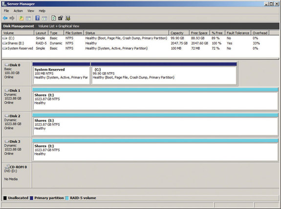
Figure 11-37 Disk Management tool of Computer Management in Windows Server 2008 R2
Windows Disk Management is not the only software RAID game in town. A number of third-party software programs work with Windows or other operating systems.
Software RAID means the operating system is in charge of all RAID functions. It works for small RAID solutions but tends to overwork your operating system easily, creating slowdowns. When you really need to keep going, when you need RAID that doesn’t even let the users know a problem has occurred, hardware RAID is the answer.
Hardware RAID centers on an intelligent controller—either a SCSI host adapter or a PATA/SATA controller that handles all of the RAID functions (see Figure 11-38). Unlike a regular PATA/SATA controller or SCSI host adapter, these controllers have chips that have their own processor and memory. This allows the card, instead of the operating system, to handle all of the work of implementing RAID.
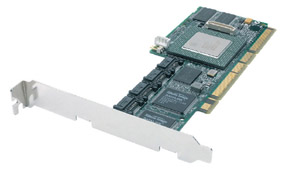
Figure 11-38 Serial ATA RAID controller
Most RAID setups in the real world are hardware-based. Almost all of the many hardware RAID solutions provide hot-swapping—the ability to replace a bad drive without disturbing the operating system. Hot-swapping is common in hardware RAID.
Hardware-based RAID is invisible to the operating system and is configured in several ways, depending on the specific chips involved. Most RAID systems have a special configuration utility in Flash ROM that you access after CMOS but before the OS loads. Figure 11-39 shows a typical firmware program used to configure a hardware RAID solution.

Figure 11-39 RAID configuration utility
Due to drastic reductions in the cost of ATA RAID controller chips, in the past few years we’ve seen an explosion of ATA-based hardware RAID solutions built into mainstream motherboards. While this “ATA RAID on the motherboard” began with parallel ATA, the introduction of serial ATA made motherboards with built-in RAID extremely common.
These personal RAID motherboards might be common, but they’re not used too terribly often given that these RAID solutions usually provide only RAID 0 or RAID 1. If you want to use RAID, spend a few extra dollars and buy a RAID 5-capable controller.
NOTE RAID controllers aren’t just for internal drives; some models can handle multiple eSATA drives configured at any of the RAID levels. If you’re feeling lucky, you can create a RAID array using both internal and external SATA drives.
RAID has been with us for about 20 years, but until only recently it was the domain of big systems and deep pockets. During those 20 years, however, a number of factors have come together to make RAID a reality for both big servers and common desktop systems. Imagine a world where dirt-cheap RAID on every computer means no one ever again losing critical data. I get goose bumps just thinking about it!
Installing a drive is a fairly simple process if you take the time to make sure you have the right drive for your system, configure the drive properly, and do a few quick tests to see if it’s running properly. Since PATA, SATA, and SCSI have different cabling requirements, we’ll look at each separately.
First, decide where you’re going to put the drive. Look for an open ATA connection. Is it PATA or SATA? Is it a dedicated RAID controller? Many motherboards with built-in RAID controllers have a CMOS setting that enables you to turn the RAID on or off (see Figure 11-40).
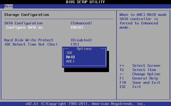
Figure 11-40 Settings for RAID in CMOS
Second, make sure you have room for the drive in the case. Where will you place it? Do you have a spare power connector? Will the data and power cables reach the drive? A quick test fit is always a good idea.
If you have only one hard drive, set the drive’s jumpers to master or standalone. If you have two drives, set one to master and the other to slave. See Figure 11-41 for a close-up of a PATA hard drive, showing the jumpers.
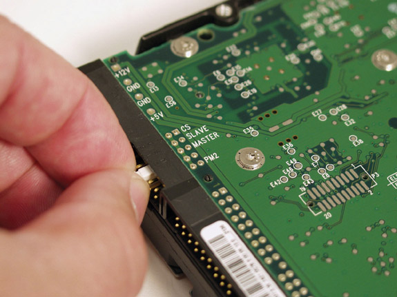
Figure 11-41 Master/slave jumpers on a hard drive
At first glance, you might notice that the jumpers aren’t actually labeled master and slave. So how do you know how to set them properly? The easiest way is to read the front of the drive; most drives have a diagram on the housing that explains how to set the jumpers properly. Figure 11-42 shows the label of one of these drives, so you can see how to set the drive to master or slave.
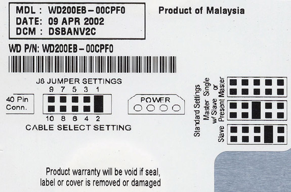
Figure 11-42 Drive label showing
Hard disk drives may have other jumpers that may or may not concern you during installation. One common set of jumpers is used for diagnostics at the manufacturing plant or for special settings in other kinds of devices that use hard drives. Ignore them; they have no bearing in the PC world. Second, many drives provide a third setting to be used if only one drive connects to a controller. Often, master and single drive are the same setting on the hard drive, although some hard drives require separate settings. Note that the name for the single drive setting varies among manufacturers. Some use Single; others use 1 Drive or Standalone.
Many PATA hard drives use a jumper setting called cable select rather than master or slave. As the name implies, the position on the cable determines which drive will be master or slave: master on the end, slave in the middle. For cable select to work properly with two drives, you must set both drives as cable select and the cable itself must be a special cable-select cable. If you see a ribbon cable with a pinhole through one wire, watch out! That’s a cable-select cable.
If you don’t see a label on the drive that tells you how to set the jumpers, you have several options. First, look at the drive maker’s Web site. Every drive manufacturer lists its drive jumper settings on the Web, although finding the information you want can take a while. Second, try phoning the hard drive maker directly. Unlike many other PC parts manufacturers, hard drive producers tend to stay in business for a long time and offer great technical support.
Hard drive cables have a colored stripe that corresponds to the number-one pin—called pin 1—on the connector. You need to make certain that pin 1 on the controller is on the same wire as pin 1 on the hard drive. Failing to plug in the drive properly will also prevent the PC from recognizing the drive. If you incorrectly set the master/slave jumpers or cable to the hard drives, you won’t break anything; it just won’t work.
Finally, you need to plug a Molex connector from the power supply into the drive. All modern PATA drives use a Molex connector.
NOTE Most of the high-speed ATA 66/100/133 cables support cable select—try one and see!
Installing SATA hard disk drives is even easier than installing PATA devices because there’s no master, slave, or cable select configuration to mess with. In fact, there are no jumper settings to worry about at all, as SATA supports only a single device per controller channel. Simply connect the power and plug in the controller cable as shown in Figure 11-43—the OS automatically detects the drive and it’s ready to go. The keying on SATA controller and power cables makes it impossible to install either incorrectly.
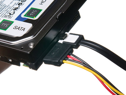
Figure 11-43 Properly connected SATA cable
The biggest problem with SATA drives is that many motherboards come with four or more. Sure, the cabling is easy enough, but what do you do when it comes time to start the computer and the system is trying to find the right hard drive to boot up? That’s where CMOS comes into play (which you’ll read about a little later).
You install a solid-state drive as you would any PATA or SATA drive. Just as with earlier hard drive types, you either connect SSDs correctly and they work, or you connect them incorrectly and they don’t. If they fail, nine times out of ten they will need to be replaced.
NOTE Installing solid-state removable media such as USB thumb drives and flash memory cards (such as SD cards) is covered in Chapter 13.
You’re most likely to run into solid-state drives today in portable computers. SSDs are expensive and offer a lot less storage capacity compared to traditional hard drives. Because they require a lot less electricity to run, on the other hand, they make a lot of sense in portable computers where battery life is essential. You can often use solid-state drives to replace existing platter-based drives in laptops.
Keep in mind the following considerations before installing or replacing an existing HDD with an SSD:
• Does the system currently use a PATA or SATA interface? You need to make sure your solid-state drive can connect properly.
• Do you have the appropriate drivers and firmware for the SSD? This is especially important if you run Windows XP. Windows Vista and 7, on the other hand, are likely to load most currently implemented SSD drivers. As always, check the manufacturer’s specifications before you do anything.
• Do you have everything important backed up? Good! You are ready to turn the system off, unplug the battery, ground yourself, and join the wonderful world of solid state.
TIP SSDs are more dependable as well as more expensive than traditional hard drives. They use less energy overall, have smaller form factors, are noiseless, and use NAND (nonvolatile flash memory) technology to store and retrieve data. They can retrieve (read) data much faster than typical HDDs.
SSDs address the many shortcomings of traditional HDDs. With solid-state technology, there are no moving metal parts, less energy is used, they come in smaller form factors, and you can access that fancy PowerPoint presentation you created and saved almost instantaneously. In geek terms, little or no latency is involved in accessing fragmented data with solid-state devices.
 CAUTION Don’t defragment an SSD! Because solid-state drives access data without having to find that data on the surface of a physical disk first, there’s never any reason to defrag one. What’s more, SSDs have a limited (albeit massive) number of read/write operations before they turn into expensive paperweights, and the defragmentation process uses those up greedily.
Connecting SCSI drives requires three things. You must use a controller that works with your drive. You need to set unique SCSI IDs on the controller and the drive. You also need to connect the ribbon cable and power connections properly.
With SCSI, you need to attach the data cable correctly. You can reverse a PATA cable, for example, and nothing happens except the drive doesn’t work. If you reverse a SCSI cable, however, you can seriously damage the drive. Just as with PATA cables, pin 1 on the SCSI data cable must go to pin 1 on both the drive and the host adapter.
NOTE Don’t let your hard drive flop around inside your case. Remember to grab a screwdriver and screw the hard drive to a slot in your case.
Every device in your PC needs BIOS support, and the hard drive controllers are no exception. Motherboards provide support for the ATA hard drive controllers via the system BIOS, but they require configuration in CMOS for the specific hard drives attached. SCSI drives require software drivers or firmware on the host adapter.
In the old days, you had to fire up CMOS and manually enter CHS information whenever you installed a new ATA drive to ensure the system saw the drive. Today, this process is automated. In fact, if you just plug in a hard drive and turn on your computer, there’s a 99 percent chance that your BIOS and OS will figure everything out for you.
As a first step in configuring controllers, make certain they’re enabled. Most controllers remain active, ready to automatically detect new drives, but you can disable them. Scan through your CMOS settings to locate the controller on/off options (see Figure 11-44 for typical settings). This is also the time to check whether your onboard RAID controllers work in both RAID and non-RAID settings.
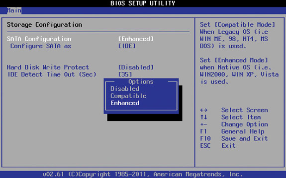
Figure 11-44 Typical controller settings in CMOS
If the controllers are enabled and the drive is properly connected, the drive should appear in CMOS through a process called autodetection. Autodetection is a powerful and handy feature that takes almost all of the work out of configuring hard drives. Here’s how it works.
One of your hard drives stores the operating system needed when you boot your computer, and your system needs a way to know where to look for this operating system. Older BIOS supported a maximum of only four ATA drives on two controllers, called the primary controller and the secondary controller. The BIOS looked for the master drive on the primary controller when the system booted up. If you used only one controller, you used the primary controller. The secondary controller was used for CD-ROMs, DVDs, or other nonbootable drives.
Older CMOS made this clear and easy, as shown in Figure 11-45. When you booted up, the CMOS queried the drives through autodetection, and whatever drives the CMOS saw, showed up here. In some even older CMOS, you had to run a special menu option called Autodetect to see the drives in this screen. There are places for up to four devices; notice that not all of them actually have a device.
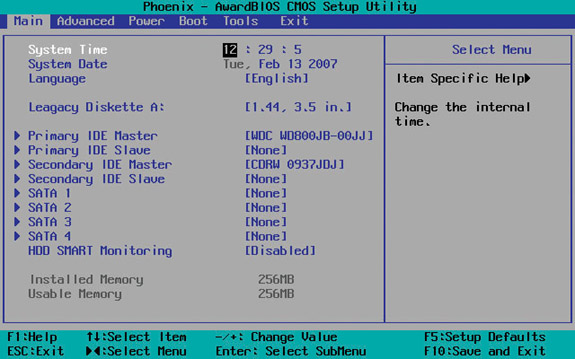
Figure 11-45 Old standard CMOS settings
The autodetection screen indicated that you installed a PATA drive correctly. If you installed a hard drive on the primary controller as master but messed up the jumper and set it to slave, it showed up in the autodetection screen as the slave. If you had two drives and set them both to master, one drive or the other (or sometimes both) didn’t appear, telling you that something was messed up in the physical installation. If you forgot to plug in the ribbon cable or the power, the drives wouldn’t autodetect.
SATA changed the autodetection happiness. The SATA world has no such thing as master, slave, or even primary and secondary controller. To get around this, motherboards with SATA use a numbering system—and every motherboard uses its own numbering system! One common numbering method uses the term channels for each controller. The first boot device is channel 1, the second is channel 2, and so on. (PATA channels may have a master and a slave, but a SATA channel has only a master, because SATA controllers support only one drive.) So instead of names of drives, you see numbers. Take a look at Figure 11-46.
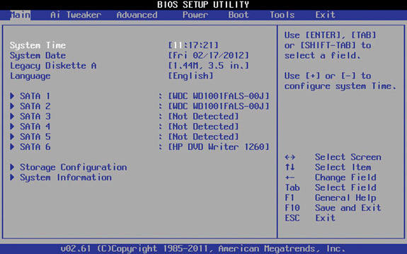
Figure 11-46 New standard CMOS features
Whew! Lots of hard drives! This motherboard supports six SATA connections. Each connection has a number, with hard drives on SATA 1 and SATA 2, and the optical drive on SATA 6. Each was autodetected and configured by the BIOS without any input from me. Oh, to live in the future!
If you want your computer to run, it’s going to need an operating system to boot. While the PCs of our forefathers (those of the 1980s and early 1990s) absolutely required you to put the operating system on the primary master, BIOS makers eventually enabled you to put the OS on any of the four drives and then tell the system through CMOS which hard drive to boot. With the many SATA drives available on modern systems, you’re not even limited to a mere four choices. Additionally, you may need to boot from an optical disc, a USB thumb drive, or even a floppy disk (if you’re feeling retro). CMOS takes care of this by enabling you to set a boot order.
NOTE Boot order is the first place to look when you see this error at boot:
Invalid Boot Disk
The system is trying to boot to a non-bootable disk. Remove any devices that might precede the desired device in the boot order.
Figure 11-47 shows a typical boot-order screen, with a first, second, and third boot option. Many users like to boot first from the optical drive and then from a hard drive. This enables them to put in a bootable optical disc if they’re having problems with the system. Of course, you can set it to boot first from your hard drive and then go into CMOS and change it when you need to—it’s your choice.

Figure 11-47 Boot order
Most modern CMOS setup utilities include a second screen for determining the boot order of your hard drives. You might want to set up a boot order that goes optical drive, followed by hard drive, and then USB thumb drive, but what if you have more than one hard drive? This screen enables you to set which hard drive goes first. If you have a different operating system on each hard drive, this can be very helpful.
On motherboards that support AHCI, you implement it in CMOS. You’ll generally have up to three options: IDE or compatibility mode, AHCI, or RAID. Use compatibility mode to install older operating systems, such as Windows XP. Going to AHCI or RAID enables the AHCI option for the HBA.
The best friend a tech has when it comes to troubleshooting hard drive installation is the autodetection feature of the CMOS setup utility. When a drive doesn’t work, the biggest question, especially during installation, is “Did I plug it in correctly?” With autodetection, the answer is simple: If the system doesn’t see the drive, something is wrong with the hardware configuration. Either a device has physically failed or, more likely, you didn’t give the hard drive power, plugged a cable in backward, or messed up some other connectivity issue.
Getting a drive installed and recognized by the system takes three or four things: jumpers (PATA only), data cable, power, and the CMOS setup recognizing the drive. If you miss or mess up any of these steps, you have a drive that doesn’t exist according to the PC! To troubleshoot hard drives, simply work your way through each step to figure out what went wrong.
First, remember to set your PATA drive to master, slave, standalone, or cable select, depending on where you decide to install it. If a drive is alone on the cable, set it to master or standalone. With two drives, one must be master and the other slave. Alternatively, you can set both drives to cable select and use a cable-select cable.
Second, you must connect the data cable to both the drive and the controller, pin 1 to pin 1. Reversing the data cable at one end is remarkably easy to do, especially with the rounded cables. They obviously don’t have a big red stripe down the side to indicate the location of pin 1! If you can’t autodetect the drive, check the cabling.
Third, be sure to give the hard drive power. PATA hard drives use a standard Molex connector, and SATA drives use the SATA power connector. If you don’t hear the whirring of the drive, make certain you plugged in a Molex from the power supply rather than from another source such as an otherwise disconnected fan. You’d be surprised how often I’ve seen that.
Fourth, you need to make sure that BIOS recognizes your hard drive. Use the CMOS setup program to check. Most of the time, however, it’s all automatic.
Once you’ve checked the physical connections, run through these issues in CMOS. Is the controller enabled? Is the storage technology—LBA, INT13, ATA/ATAPI-6—properly set up? Similarly, can the motherboard support the type of drive you’re installing? If not, you have a couple of options. You can either flash the BIOS with an upgraded BIOS from the manufacturer or get a hard drive controller that goes into an expansion slot.
Finally, with nonintegrated hard drive controllers such as those that come with many SATA drives, make certain that you’ve installed the proper drivers for the controller. Driver issues can crop up with new, very large drives and with changes in technology. Always check the manufacturer’s Web site for new drivers.
Windows Vista and Windows 7 support hybrid hard drives (HHDs), drives that combine flash memory and spinning platters to provide fast and reliable storage, and offer ReadyBoost for faster caching and booting. Samsung has drives with 128-MB and 256-MB flash cache, for example, that shave boot times in half and, because the platters don’t have to spin all of the time, add 20-30 minutes more of battery life for portable computers. Adding that much more run time with only a tiny price premium and no extra weight is the Holy Grail of portable computing.
1. John’s system is running INT13 extensions. What is the maximum size hard drive it can support?
A. 504 GB
B. 137 GB
C. 10 GB
D. 8.4 GB
2. How many PATA hard drives can you have on a system with two PATA hard drive controllers?
A. 1
B. 2
C. 3
D. 4
3. How do you differentiate two PATA drives on the same cable?
A. The flat ribbon cable has a seven-wire twist that determines which is which.
B. You set jumpers on the individual drives to determine which is master and which is slave.
C. The PATA controller determines the hierarchy.
D. Both drives are considered equal.
4. What happens if you cable a PATA hard drive incorrectly?
A. You can destroy that hard drive.
B. The data will be erased, but the hard drive will be okay.
C. The system will not be able to communicate with that hard drive.
D. Nothing. It doesn’t matter how the cable is set up; it doesn’t have the seven-wire twist.
5. John needs to install an old ATA/100-capable hard drive to check the contents before recycling it. Looking through his box of connectors, however, he finds no 80-wire cable, just a 40-wire cable. If he installs the ATA/100 drive with a 40-wire EIDE cable, what will happen?
A. The drive will work but will not run at the ATA/100 speed.
B. He might damage the motherboard.
C. He won’t be able to install the drive, because the cables are incompatible.
D. He will not be able to run in ATA mode.
6. What is the maximum cable length of an internal SATA device?
A. 2 meters
B. 12 inches
C. 18 inches
D. 1 meter
7. Which of the following is part of the ATA-7 standard?
A. Red controller connections on the motherboard
B. SATA
C. ATA/100
D. 1 meter maximum cable length
8. What is the maximum number of SATA drives you can have on a system?
A. One master, one slave
B. Two, with no master/slave distinction
C. Eight
D. There is no maximum other than the limitations of your motherboard.
9. Simon wants to connect his old PATA hard drive to the SATA controller in his new computer. What does he need to do this?
A. He needs a SATA bridge to plug into the connector on the PATA drive.
B. He needs a PATA converter to plug into the SATA bridge on the controller.
C. Nothing at all; he can just connect the PATA drive directly to the SATA controller.
D. He can’t do it; the SATA controller is not backward compatible with PATA drives.
10. What do you call a series of SCSI devices working together through a host adapter?
A. A SCSI controller
B. A SCSI chain
C. RAID
D. Cabled SCSI
1. B. A system running INT13 extensions can support up to a 137-GB hard drive.
2. D. Each controller supports two drives.
3. B. PATA drives use master/slave jumpers to differentiate between the two drives.
4. C. Nothing will be damaged or lost—there just won’t be any communication.
5. A. ATA/100 drives work fine with a 40-wire cable—they just won’t run at ATA/100 speed.
6. D. The maximum cable length of an internal SATA device is 1 meter.
7. B. Serial ATA is part of the ATA-7 standard.
8. D. There is no maximum number of SATA drives you can have on a system beyond the limits imposed by the number of ports on your motherboard/host card.
9. A. Simon needs a SATA bridge to plug into the connector on the PATA drive to connect his old PATA hard drive to the SATA controller.
10. B. A series of SCSI devices working together through a host adapter is a SCSI chain.