Methods That Measure and/or Manipulate Biological Forces or Use Forces in Their Principle Mode of Operation on Biological Matter
What would happen if we could arrange the atoms one by one the way we want them?
— Richard Feynman, Physicist (1959)
General Idea: Several biophysical methods can both measure and manipulate biological forces across a range of length and time scales. These include methods that characterize forces in whole tissues, down through to single cells and to structures inside cells, right down to the single-molecule level. The force fields that are generated to probe the biological forces originate from various sources including hydrodynamic drag effects, solution pressure gradients, electrical attraction and repulsion, molecular forces, magnetism, optical forces, and mechanical forces. All of which are explored in this chapter.
All experimental biophysical techniques clearly involve measurement and application of forces in some form or another. However, there is a subset of methods that are designed specifically to either measure the forces generated in biological systems, or to control and manipulate them. Similarly, there are tools that do not characterize biological forces directly, but which primarily utilize force methods in their mode of operation, for example, in using pressure gradients to purify biomolecular components.
There now exist several methods that permit both highly controlled measurement and manipulation of the forces experienced by single biomolecules. These various tools all come under the banner of force transduction devices; they convert the mechanical molecular forces into some form of amplified, measurable signal. Many of these single-molecule force techniques share several common features, for example, single molecules are not in general manipulated directly but are in effect physically conjugated, usually via one or more chemical links, to some form of adapter that is the real force transduction element in the system. The principle forces that are used to manipulate the relevant adapter include optical, magnetic, electrical, and mechanical. These are all coupled into an environment of complex feedback electronics and stable, noise-minimizing microscope stages, both for purposes of measurement and for manipulation.
Single-molecule biophysics methods extend beyond just force tools, which we explore here, encompassing also a range of advanced imaging techniques that we explored previously in Chapters 3 and 4. However, an important point to note here about single-molecule methods concerns the ergodic hypothesis of statistical thermodynamics. The ergodic hypothesis maintains that there is an equivalence between ensemble and single-molecule properties. In essence, over long periods of time, all accessible microstates are equally probable. This means that an ensemble average measurement (e.g., obtained from the mean average from many thousands of molecules) will be the same as the time-averaged measurement taken from one single molecule over a long period of time. The key difference with a single-molecule experiment is that one can sample the whole probability distribution of all microstates as opposed to just determining the mean value from all microstates as is the case from a bulk ensemble average experiment, though the caveat is that in practice this often involves generating significant amounts of data from single-molecule experiments to properly sample the underlying probability distribution.
KEY POINT 6.1
The ergodic hypothesis, that all accessible microstates are equally probable over a long time, is relevant to single-molecule methods since it implies that the population mean measurement from a bulk ensemble experiment, involving typically several thousand molecules or more, will be the same as the mean of several measurements made on a single molecule sampled over a long period of time.
Statistical thermodynamics implicitly assumes ensemble average parameters. That is, a system with many, many particles. For example, a single microliter of water contains ~1019 molecules. To apply the same concepts to a single molecule requires the ergodic hypothesis.
Intuitively, one might think that the mean average property of thousands upon thousands of molecules is an adequate description for any given single molecule. In some very simple, or exceptional, molecular systems, this is in fact the case. However, in general, this is not strictly true. The reason is that single biomolecules often exist in multiple microstates, which is in general intrinsically related to their biological function. A microstate here is essentially a measure of the free energy locked into that molecule, which is a combination of mainly chemical binding energy, the so-called enthalpy, and energy associated with how disordered the molecule is, or entropy. There are many molecules that, for example, exist in several different spatial conformations; a good illustration of which are molecular machines, whose theory of translocation is discussed later in Chapter 8. In other words, the prime reason for studying biology at the level of single molecules is the prevalence of molecular heterogeneity.
In the case of molecular machines, although there may be one single conformation that has a lower free energy microstate than the others, and thus is the most stable, several other shorter-lived conformations exist that are utilized in different stages of force and motion generation. The mean ensemble average usually looks similar to the most stable of these different conformations, but this single average parameter tells us very little of the behavior of the other shorter lived but functionally essential conformational states. What cannot be done with bulk ensemble average analysis is to probe such multistate molecular systems. The power of single-molecule experiments is that these subpopulations of molecular microstates can be explored directly and individually. Such subpopulations of states are a vital feature of the proper functioning of natural molecular machines.
As discussed in Chapter 2, there is a fundamental energetic instability in molecular machines, which allows them to switch between multiple states as part of their underlying physiological function. There are however many experimental biophysical methods that can be employed in bulk ensemble investigations to synchronize a molecular population. For example, these include thermal and chemical jumps such as stopped-flow reactions, electric and optical methods to align molecules, as well as freezing and/or crystallizing a population. A risk with such approaches is that the normal physiological functioning may be different. Some biological tissues, for example, muscles and cell membranes, are naturally ordered on a bulk scale. It is thus no mystery why these have historically generated the most physiologically relevant ensemble data.
The lack of temporal and/or spatial synchronicity in ensemble average experiments is the biggest challenge in obtaining molecular level information. Different molecules in a large population may be doing different things at different times. For example, molecules may be in different conformational states at any given time, so the mean ensemble average snapshot encapsulates all temporal fluctuations resulting in a broadening of the distribution of whatever statistical parameter is being measured. A key problem of molecular asynchrony is that a typical ensemble experiment is in steady state. That is, the rate of change between forward and reverse molecular states is the same. If the system is momentarily taken out of steady state, then transient molecular synchrony can be obtained, for example, by forcing all molecules into just one state; however, this by definition is a short-lived effect, so practical measurements are likely to be very transient.
Some ensemble average techniques overcome this problem by forcing the majority of the molecules in a system a single microstate, for example, with crystallography. But in general this widening of the measurement distribution presents challenges of result interpretation since there is no easy way to discriminate between anticipated widening of an experimental measurement due to, for example, finite detector sensitivity, and the more biologically relevant widening of the distribution due to underlying molecular asynchrony.
Thermal fluctuations in the surrounding solvent water molecules often act as the driving force for molecular machines switching between different states. This is because the typical energy difference between different molecular microstates is very similar to the thermal scale of ~kBT energy associated with any molecule coupled to the thermal reservoir at a given temperature. However, it is not so much the heat energy of the biomolecule itself, which drives change into a different state, but rather that associated with each surrounding water molecule. The density of water molecules is significantly higher in general than that of the biomolecules themselves, so each biomolecule is bombarded by frequent collisions with water molecules (~109 per second), and this change of momentum can be transformed to mechanical energy of the biomolecule. This may be sufficient to drive a change of molecular state. Biomolecules are thus often described as existing in a thermal bath.
There is a broad range in concentration of biomolecules inside living cells, though the actual number directly involved in any given biological process at any one time is generally low. Biological processes occur under typically minimal stoichiometry conditions in which stochastic molecular events become important. Paradoxically, it can often be these rarer, single-molecule events that are the most significant to the functioning of cellular processes. It becomes all the more important to strive to monitor biological systems at the level of single molecules.
KEY POINT 6.2
Temporal fluctuations in biomolecules from a population result in broadening the distribution of a measured parameter from an ensemble average experiment, which can be difficult to interpret physiologically. Thermal fluctuations are driven primarily by collisions from surrounding water molecules, which can drive biomolecules into different microstates. In an ensemble average experiment, this can broaden the measured value, which makes reliable inference difficult.
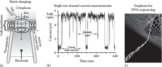
Single-molecule force methods include variants on optical tweezers and magnetic tweezers designs. They also include scanning probe microscopy (SPM) methods, the most important of which in a biophysical context is atomic force microscopy (AFM), which can be utilized both for imaging and in force spectroscopy. Electrical forces in manipulating biological objects, from molecules through to cells, are also relevant, such as for electric current measurements across membranes, for example, in patch clamping. On a larger length scale, rheological and hydrodynamic forces form the basis of several biophysical methods. Similarly, elastic forces are important components of techniques that permit whole cells and tissues to be mechanically probed.
6.2 RHEOLOGY AND HYDRODYNAMICS TOOLS
Rheology is the study of matter flow, principally in a liquid state. For the investigation of living matter, the liquid state is primarily concerned with water, namely, hydrodynamics forces especially those that operate primarily through viscous drag forces on biological material, but is also concerned with the force response of fluid states of cellular structures. For example, how lipid membranes in cells, which have many properties consistent with those of liquid crystals, respond to external force and also how components inside the cell membrane impart rheological forces on neighboring components. In this section, we discuss a range of hydrodynamics force techniques used to study biological matter, as well as rheological force methods for probing cellular liquid/soft-solid states. These include a range of standard but invaluable tools (e.g., chromatography can arguably be considered a rheological force method) and also methods that utilize centrifugation and osmosis to characterize and/or isolate biological components. We also discussed techniques that result in plastic/viscoelastic rheological deformation of biological soft matter in response to applied forces.
6.2.1 CHROMATOGRAPHY TECHNIQUES
Chromatography is a standard biophysical tool used to separate components in an in vitro biological sample on the basis of different molecular properties such as mass and charge. In many biochemistry textbooks, this might not be considered in the context of being a “force method”; however, it does rely on a range of cohesive forces in water in particular, and so we discussed it here. Related methods include high-performance liquid chromatography, gas chromatography, gel filtration, thin-layer chromatography, and even standard paper chromatography. Molecular components bind to an immobile substrate to form a stationary phase for a characteristic dwell time, dependent on the physical and chemical features nature of the substrate. The mobile phase moves through the chromatography device via diffusion often facilitated by a driving pressure gradient.
Sepharose beads (sepharose is the trade name of a type of polysaccharide sugar generically called agarose, which is purified from seaweed and used for several purposes in experimental biology) of diameter ~40–400 μm are often used as the immobile substrate, tightly packed into a glass column for gel filtration chromatography and related affinity chromatography that uses specific antibodies bound to the beads, or different bead surface charges in ion-exchange chromatography. These factors, in addition to chemical parameters of the media in the mobile phase such as pH and ionic strength, determine the dwell time in the stationary phase, and thus the mean drift speed of each molecular component through the device. The end result is to separate out different molecular components on the basis of their relative binding strengths to the immobile substrate and of their mean speed of translocation through the chromatography device, with emerging components often detected using an optical absorption technique at a specific wavelength.
Size exclusion chromatography (SEC) is a chromatography method in which molecules in solution are separated on the basis of their size, and/or molecular weight, usually applied to large molecules such as proteins and nucleic acids. In SEC, a small molecule can penetrate more regions of the stationary phase pore system compared to larger molecules and so will have a slower drift speed thus enabling larger and smaller molecules to emerge as different fractions at the bottom of a gel filtration column.
Reversed phase chromatography uses an electrically polar aqueous mobile phase and a hydrophobic stationary phase. Hydrophobic molecules preferentially adsorb to this stationary phase, and thus hydrophilic molecules have a faster drift speed in the mobile phase and will elute first from the bottom of the column. This enables separation of hydrophobic and hydrophilic biomolecules.
Sedimentation methods can be used to purify and characterize different components in in vitro biological samples. They rely on the formation of a sedimented pellet when it is spun in a centrifuge, depending on the frictional viscous drag of the sample and its mass. Quantitative measurements may be made using analytical ultracentrifugation, which generates centripetal forces ~300,000 times that of gravity and also have controlled cooling to avoid localized heating in the sample, which may be damaging in the case of biological material. By estimating the sedimentation speed, we can infer details of the size and shape of biological molecules and large complexes of molecules, as well as their molecular mass. Balancing the centripetal force on a particle of mass m being spun at angular velocity ω at a radius r from the axis of rotation with the buoyancy force from the displacement of the solvent by the particle and the viscous drag force due to moving through the solution with sedimentation speed v leads to a relation for the sedimentation coefficient s:
(6.1) |
where
ρ is the density
γ is the frictional drag coefficient
Diffusion causes the shape of the sedimenting boundary of the spun solution to spread with time. This can be monitored using either optical absorption or interference techniques, allowing both the sedimentation coefficient and the translation diffusion coefficient D to be determined. The Stokes–Einstein relationship (see Chapter 2) is then used to determine γ from D, which can be used to estimate the molecular mass.
A mix of different biological molecules (e.g., several different enzymes) may sometimes be separated on the basis of sedimentation rates in a standard centrifugation device, and a density gradient of suitable material (sucrose and cesium chloride are two commonly used agents) is created, such that there is a higher density of that substance toward the bottom of a centrifuge tube. By centrifuging the mix into such a gradient, the different chemicals may separate out as bands at different heights in the tube and subsequently be extracted as appropriate.
Field flow fractionation is a hydrodynamic separation technique that involves forward flow of a suspension of particles in a sample flow cell plus an additional hydrodynamic force applied normal to the direction of this flow. This perpendicular force is typically provided by centrifugation of the whole sample flow cell. Particles with a higher sedimentation coefficient will drift toward the edge of the flow cell due to this perpendicular force more rapidly than particles with a lower sedimentation coefficient. Under nonturbulent laminar flow conditions, known as “Poiseuille flow” (see Chapter 7) in a typical cylindrical-shaped pipe containing the sample, the speed profile of the fluid normal to the pipe long axis is parabolic (i.e., maximum in the center of the pipe, zero at the edges); thus, the particles with higher sedimentation coefficients are shifted more from the fastest on-axis flow lines on the pipe and will have a smaller drift speed through the flow cell. This therefore enables particles to be separated on the basis of sedimentation coefficient—put simply, to separate larger from smaller particles.
Microfluidics can use these principles to separate out different biological components on the basis of flow properties. Here, flow channels are engineered to have typical widths on the length scales of a few tens of microns, and different channels can be connected to generate a complex flow-based device. These systems are discussed fully in Chapter 7.
6.2.3 TOOLS THAT UTILIZE OSMOTIC FORCES
Dialysis, or ultrafiltration, has similar operating principles to chromatography in that the sample mobility is characterized by similar factors, but the solvated sample is on one side of a dialysis membrane that has a predefined pore size. This sets an upper molecular weight limit for whether molecules can diffuse across the membrane.
This selectively permeable membrane (also referred to as a semipermeable membrane) results in an osmotic force driven by entropy. On either side of the membrane, there is a concentration gradient, that is, the concentration of solvated molecules on one side of the membrane is different from that on the other side. The water molecules in the solution that has a higher concentration have more overall order since there are a greater relative number of available solute molecules to which they bond, usually via electrostatic and/or hydrogen bonding. This entropy difference between the two solutions either side of the membrane is manifested as a statistical/entropic driving force when averaged over time scales are much larger than the individual water molecule collision time, which acts in a direction to force a net flux of water molecules from the low-to high-concentration solutions (note that this is also the physical basis of Raoult’s law, which states that the partial vapor pressure of each component of an ideal mixture of liquids is equal to the vapor pressure of the pure component multiplied by its mole fraction in that mixture). This process can be used to separate different populations of biomolecules of the basis of molecular weight, often facilitated by a pressure gradient. The use of multiple dialysis stages using membranes with different pore sizes can be used to purify a complex mix of different molecules.
Osmotic pressure can also be used in the study of live cells. Lipid membranes of cells and subcellular cell organelles are selectively permeable. Although some ions undergo passage diffusion through pores in the membrane, in general the passage of water, ions, and various biomolecules is highly selective and often tightly regulated. Enclosure of solutes inside a cell membrane therefore results in a strong osmotic pressure on cells, exerted from the inside of the cell onto the membrane toward the outside.
As discussed previously (see Chapter 2), there are various mechanisms to prevent cells from exploding due to this osmotic pressure depending on the cell type, for example, cell walls in bacteria and plant cells, and/or regulation of ion and water pumps that are especially important in eukaryotic cells that in general have no stiff cell wall barrier. These mechanisms can be explored in an osmotic chamber. This is a device that allows cells to be visualized using light microscopy in their normal aqueous environment but allowing the external pressure exerted through the liquid environment to be carefully controlled, up to pressures or several tens of atmospheres. Combining cellular pressure control with fluorescence microscopy to probe cell wall proteins and ion channel components has proved informative to our understanding of cellular osmoregulatory mechanisms.
6.2.4 DEFORMING BIOLOGICAL MATTER WITH FLOW
Aqueous flow can be used to straighten relatively long, filamentous biomolecules in a process called molecular combing. For example, by attaching one end of the molecule to a microscope coverslip using specific antibody binding or a specific chemical conjugation group on the end of the molecule, very gentle fluid flow is sufficient to impart enough viscous drag on the molecule to extend it parallel to the direction of flow (for a theoretical discussion of the mechanical responses of biopolymers to external forces, see Chapter 8).
This technique has been applied to filamentous protein molecules such as titin, a large muscle protein discussed later in this chapter in the context of single-molecule force transduction techniques, which can then facilitate imaging of the full extent of the molecule, for example, using fluorescence imaging if fluorophore probes can be bound to specific regions of the molecule, or using transmission electron microscopy. Binding a micron-sized bead to the other end of the molecule increases the viscous drag in the fluid flow and allows higher forces to be exerted on the molecule, and thus larger molecular extensions. This has been used on single DNA molecules in vitro, for example, in the study of DNA replication. This technique of extending a biomolecule-tethered bead by flow can also be used in conjunction with optical and magnetic tweezers to facilitate the initial stable trapping of the bead.
The molecular combing technique can be adapted to significantly improve throughput. This is seen most dramatically in the DNA curtains technique (Finkelstein et al., 2010). Here, DNA molecules are tethered on a nanofabricated microscope coverslip containing etched platforms for tether attachment such that the tethered end of a molecule is clear from the coverslip surface, thus minimizing the effects of surface forces on the molecule, which are often difficult to quantify and can impair the biological function of DNA. Optimization of the tethering incubation conditions allows several individual DNA molecules to be tethered in line, spaced apart on the coverslip surface by only a few hundred nm.
The molecules can be visualized by labeling the DNA using a range of DNA-binding dyes and imaging the molecules in real time using fluorescence microscopy. This can be used to investigate the topological, polymer physics properties of single DNA molecules, but can also be used in investigating a variety of different molecular machines that operate by binding to DNA by labeling a component of the machine with a different color fluorophore and then utilizing dual-color fluorescence imaging to monitor the DNA molecules and molecular machines bound to them simultaneously. The key importance of this technique is that it allows several tens of individual DNA molecules to be investigated simultaneously under the same flow and imaging conditions, improving statistical sampling, and subsequent biological interpretation of the data, enormously.
KEY BIOLOGICAL APPLICATIONS: RHEOLOGYTOOLS
Molecular separation and identification.
There are several biophysical techniques that utilize the linear momentum associated with a single photon of light, to generate forces that then can be used to probe and manipulate single biomolecules and even whole cells. Optical tweezers utilize this approach, as do the related optical stretcher technology. Optical tweezers are an exceptionally powerful tool for manipulating single biomolecules and characterizing many aspects of their force-dependent features, and for this reason we explore the theory of their operation in detail here. Although single biomolecules themselves cannot be optically trapped with any great efficiency (some early optical tweezers experiments toyed with rather imprecise manipulation of chromosomes), they can be manipulated via a micron-sized optically trapped bead. But there are also methods that can utilize the angular momentum of photons to probe rotary motion of biological material. Other applications of optics, which allow monitoring of biological forces, include Brillouin scattering, polarization microscopy, and Förster resonance energy transfer (FRET).
6.3.1 BASIC PRINCIPLES OF OPTICAL TWEEZERS
The ability to trap particles using laser radiation pressure was reported first by Arthur Ashkin, the pioneer of optical tweezers (also known as laser tweezers) (Ashkin, 1970). This was a relatively unstable 1D trap consisting of two juxtaposed laser beams whose photon flux resulted in equal and opposite forces on a micron-sized glass bead. The modern form of the standard 3D optical trap (specifically described as a single-beam gradient force trap), developed in the 1980s by Ashkin et al. (1986), results in a net optical force on a refractile, dielectric particle, which has a higher refractive index than the surrounding medium, roughly toward the intensity maximum of a focused laser. These optical force transduction devices have since been put to very diverse applications for the study of single-molecule biology (for older but still rewarding reviews, see Svoboda and Block, 1994 for an accessible explanation of the physics, and Moffitt et al., 2008 for a compilation of some of the applications).
Photons of light carry linear momentum p given by the de Broglie relation p = E/c = hν/c = h/λ, for a wave of energy E, frequency ν, and wavelength λ where c is the speed of light and h Plank’s constant. Photon momentum results in radiation pressure if photons are scattered from an object. Also, if refraction occurs at the point of a photon emerging from an optically transparent particle, there is a change in beam direction and intensity, and thus a change in momentum, which results in an equal and opposite force on the particle. Standard optical tweezers utilize this effect as a gradient force in the focal plan of a light microscope.
KEY POINT 6.3
Basics of optical tweezers:
1. If a refractile particle changes the direction of a photon, then a force acts on it according to Newton’s third law, since photons have momentum.
2. The intensity to generate optical forces large enough to overcome thermal forces at room temperature is high and so requires a laser.
3. If a laser beam is brought to a steep focus, the combination of scatter and refractive force results in a net force roughly toward the laser focus.
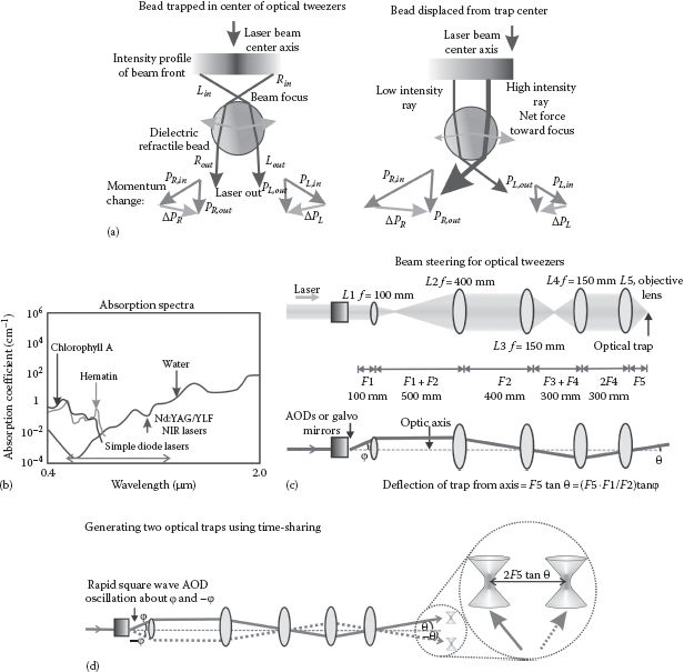
To understand the principles of optical trapping, we can consider the material in the particle through which photons propagate to be composed of multiple electric dipoles on the same length scale as individual atoms. A propagating electromagnetic light wave through the particle imparts a small force on each electric dipole which time averages to point in the direction of the intensity gradient of the photon beam. A full derivation of the forces involved requires a solution of Maxwell’s electromagnetic equations (see Rohrbach, 2005); however, we can gain qualitative insight by considering a ray-optic depiction of the passage of light through a particle (Figure 6.1a).
FIGURE 6.1 (See color insert.) Optical tweezers. (a) The sum of refractive forces through a bead in optical tweezers results in a net force roughly toward the laser focus. (b) Many biomolecules indicate strong absorption in the visible light range, illustrated here with chlorophyll in plants and hematin in the blood; water absorbs weakly in the visible, increasing absorption in the near infrared, but with a local dip in absorption at ~1 μm wavelength. (c) Typical arrangement for beam steering (and expansion) for optical tweezers. (d) Two (or more) optical traps can be generated by time-sharing of the laser beam using rapid deflection by an AOD.
The photon energy flux dE in a small time dt of a laser beam parallel to the optic (z) axis of total power P propagating through the particle is given by
(6.2) |
where
c is the speed of light
p is the total momentum of the beam of photons, such that dp is the small associated change in momentum in time dt
If we assume that the lateral optical trapping force F arises mainly from photons traveling close to the optic axis, which is exerted as photons exit the particle at a slightly deviated direction from the incident beam by a small angle θ, then F is given by the rate of change of photon momentum projected onto the x-axis:
(6.3) |
where, we assume the small-angle approximation if θ is measured in radians. Typically, for optical tweezers θ will be a few tens of milliradians, equivalent to a few degrees (see Worked Case Example 6.1).
Typically, a single-mode laser beam (the so-called TEM00 that is the lowest-order fundamental transverse mode of a laser resonator head and has a Gaussian intensity profile across the beam) is focused using a high NA objective lens onto a refractile, dielectric particle (typically a bead of diameter ~10−6 m composed of latex or glass) whose refractive index (~1.4–1.6) is higher than that of the surrounding water solution (~1.33), to form a confocal intensity volume (see Chapter 4). Optical trapping does not require symmetrical particles though most often the particles used are spheres. A stably trapped particle is located slightly displaced axially by the forward scatter momentum from the laser focus, which is the point at which the gradient of the intensity of the focused laser light in the lateral xy focal plane of the microscope is zero.
If the particle is displaced laterally from the focus, then the refraction of the higher-intensity light fraction through the particle close to the focus causes an equal and opposite force on the particle, which is greater than that experienced in the opposite direction due to refraction of the lower-intensity portion of the laser beam. The particle therefore experiences a net restoring force back to the laser focus and hence is “trapped,” providing any external force perturbations on the particle do not displace it beyond the physical extent of the optical tweezers.
In practice, stable optical tweezers require a diffraction-limited focus; photons entering the focal waist of the confocal volume at a steep angle relative to the optical axis result in high-intensity gradients across the trap profile and so contribute the most to the optical restoring force. To achieve this steepness of angle requires a high NA objectives lens in the range ~1.2–1.5 often combined with marginally overfilling the back aperture of the objective lens with collimated incident laser light. The actual size of the optical tweezers trapping volume is determined by the spatial extent of the diffraction-limited interference pattern in the vicinity of the laser focus, which laterally (xy) has a width of ~λ, whereas axially (z) this is more like ~2–3 times λ (see Chapter 4). This implies that the intensity gradient is reduced by the same factor. Combining this reduction in axial gradient stiffness with a weakness of the axial trapping force due to forward scatter radiation pressure results in axial trap stiffness values (i.e., a measure of the restoring force for a given small displacement of the particle) that are smaller than the lateral stiffness by a factor of ~3–8, depending on the particle size and specific wavelength used.
6.3.2 OPTICAL TWEEZERS DESIGNS IN PRACTICE
Typical bead diameters are ~0.2–2 μm, though optical trapping has been demonstrated on gold-coated particles with a diameter as small as 18 nm (Hansen et al., 2005). The wavelength used is normally near infrared (NIR) of ~1 μm, the choice being made on the basis of optimization of trap stiffness and size while minimizing sample photodamage. Some damage is due to a localized heating effect from laser absorption either by the water solvent or chromophores in the biological sample, at a level of ~1–2 K for every 100 mW of NIR laser power. However, the most likely cause of biological damage is due to the generation of free radicals in the water through single- and multiphoton absorption effects found at high local intensities at the focus of a trap, which can bind indiscriminately to biological structures.
The choice of wavelength used is a compromise between two competing absorption factors. One is that absorption of electromagnetic radiation by water itself increases sharply from visible into the infrared, peaking at a wavelength of ~3 μm. However, natural biological chromophores can absorb strongly at visible light wavelengths, as well as increasing the likelihood for generating free radicals; therefore, a wavelength of ~1 μm is a good compromise. At wavelengths between 1 and 1.2 μm, there is also a small local dip in the water absorption spectrum, which makes Nd:YAG (λ = 1.064 μm) and Nd:YLF (λ = 1.047 μm) crystal lasers attractive choices (Figure 6.1b).
In most applications, optical tweezers are coupled to a light microscope. An NIR laser beam is expanded usually to marginally overfill the back aperture of a high NA objective lens, which is steered by upstream optics to rotate the beam through the back aperture, resulting in lateral displacement of the optical trap at the focal plane in a microscope flow cell (Figure 6.1c). Steering of the optical trap can be done using mirrors positioned in a conjugate plane to the objective lens back aperture. However, it is common in many applications to use higher bandwidth steering with acousto-optic deflectors (AODs), discussed in the following text. The laser beam for generating a conventional gradient force optical trap can be split before reaching the sample, either using a space-dividing optical component such as a glass splitter cube or by time-sharing the beam along different optical paths in the microscope setup, to generate more than one optical tweezers (Figure 6.1d). Time-sharing is most popularly obtained by passing the initial beam through AODs.
An AOD is composed of an optical crystal, typically of tellurium dioxide (TeO2) in a synthetic tetragonal structure (also known as the crystal paratellurite). In this form, TeO2 is a nonlinear optical crystal that is transparent through the visible and into the mid-infrared range of the electromagnetic spectrum, with a high refractive index of ~2.2, exhibiting a relatively slow shear-wave propagation along the [110] crystal plane. These crystals exhibit photoelasticity, in that mechanical strain in the crystal results in a local change in optical permittivity, manifest as there being a spatial dependence on refractive index. These factors facilitate standing wave formation in the crystal parallel to the [110] plane from acoustic vibration if a radio frequency forcing function is applied from a piezoelectric transducer from one end of the crystal, with the other end of the crystal at the far end of the [110] plane acting as fixed point in being coupled to an acoustic absorber (Figure 6.2a). The variation in refractive index can be modeled as
(6.4) |
where
n0 is the unstrained refractive index
ω is the angular frequency of the forcing function
k is the wave vector of the sound wave parallel to the z-axis (taken as parallel to the [110] plane)
The factor Δn is given by the photoelastic tensor parameters. The result is a sinusoidally varying function of n with a typical spatial periodicity of around a few hundred nm, which thus has similar attributes to a diffraction grating for visible/infrared light. The diffracted light is a mixture of two types, that due to Raman–Nath diffraction, which can occur at an arbitrary angle of incidence at lower acoustic frequencies (most prevalent at ~10 MHz or less), and that due to Bragg diffraction (see Chapter 4) at higher acoustic frequencies more typically >100 MHz, which occurs at a specific angle of incident θB such that
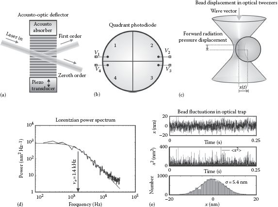
FIGURE 6.2 Controlling bead deflections in optical tweezers. (a) In an AOD, radio-frequency driving oscillations from a piezo transducer induce a standing wave in the crystal that acts as diffraction grating to deflect an incident laser beam. (b) Schematic of sectors of a quadrant photodiode. (c) Bead displacement in optical tweezers. (d) Bead displacements in an optical trap, here shown with a trap of stiffness 0.15 pN/nm, have a Lorentzian-shaped power resulting in a characteristic corner frequency (here 1.4 kHz) that allows the trap stiffness to be determined, which can also be determined from (e) the root mean squared displacement, shown here for data of the same trapped bead (see Leake, 2001).
(6.5) |
where
λ is the free-space wavelength of the incident light
f is the acoustic wave frequency
ni and nd are the incident and diffracted wave refractive indices of the medium, respectively
v is the acoustic wave speed
AODs are normally configured to use the first-order Bragg diffraction peak angle θd for beam steering, which satisfies sin(θd) = λ/Λ where Λ is the acoustic wavelength. The maximum efficiency of an AOD is ~80% in terms of light intensity propagated into the first-order Bragg diffraction peak (the remainder composed of Raman–Nath diffraction and higher-order Bragg peaks), and for steering in the sample focal plane in both x and y requires two orthogonal AODs; thus, ~40% of incident light is not utilized, which can be disadvantageous if a very high stiffness trap is desired.
An AOD has a frequency response of >107 Hz, and so the angle of deflection can be rapidly alternated between ~5° and 10° on the submicrosecond time scale resulting in two time-shared beams separated by a small angle, that can then each be manipulated to generate a separate optical trap. Often, two orthogonally crossed AODs are employed to allow not only time-sharing but also independent full 2D control of each trap in the lateral focal plane of the microscope, over a time scale that is ~3 orders of magnitude faster than the relaxation time due to viscous drag on a micron-sized bead. This enables feedback type experiments to be applied. For example, if there are fluctuations to the molecular force of a tethered single molecule then the position of the optical trap(s) can be rapidly adjusted to maintain a constant molecular force (i.e., generating a force clamp), which allows, for example, details of the kinetics of molecular unfolding and refolding to be explored in different precise force regimes.
An alternative method to generating multiple optical traps involves physically splitting the incident laser beam into separate paths using splitter cubes that are designed to transmit a certain proportion (normally 50%) of the beam and reflect the remainder from a dielectric interface angled at 45° to the incident beam so as to generate a reflected beam path at 90° to the original beam. Other similar optical components split the beam on the basis of its linear polarization, transmitting the parallel (p) component and reflecting the perpendicular (s) component, which has an advantage over using nonpolarizing splitter cubes in permitting more control over the independent laser powers in each path by rotating the incident E-field polarization vector using a half-wave plate (see Chapter 3). These methods can be used to generate to independently steerable optical traps.
The same principle can be employed to generate >2 optical traps; however, in this case, it is often more efficient to use either a digital micromirror array or a spatial light modulator (SLM) component. Both optics components can be used to generate a phase modulation pattern in an image plane conjugate to the Fourier plane of the sample’s focal plane, which results in controllable beam deflection into, potentially, several optical traps, which can be manipulated not only in x and y but also in z. Such approaches have been used to generate tens of relatively weak traps whose position can be programmed to create an optical vortex effect, which can be used to monitor fluid flow around biological structures. The primary disadvantage of digital micromirror array or SLM devices is that they have relatively low refresh bandwidths of a few tens of Hz, which limit their utility to monitoring only relatively slow biological processes, if mobile traps are required. But they have an advantage in being able to generate truly 3D optical tweezers, also known as holographic optical traps (Dufresne and Grier, 1998).
Splitting light into a number of N traps comes with an obvious caveat that the stiffness of each trap is reduced by the same factor N. However, there are many biological questions that can be addressed with low stiffness traps, but the spatial fluctuations on trapped beads can be >10 nm, which often swamps the molecular level signals under investigation. The theoretical upper limit to N is set by the lowest level of trap stiffness, which will just be sufficient to prevent random thermal fluctuations pushing a bead out of the physical extent of the trap. The most useful multiple trap arrangement for single biomolecule investigations involves two standard Gaussian-based force gradient traps, between which a single biomolecule is tethered.
6.3.3 CHARACTERIZING DISPLACEMENTS AND FORCES IN OPTICAL TWEEZERS
The position of an optically trapped bead can be determined using either the bright-field image of the bead onto a charge-coupled device (CCD) camera or quadrant photodiode (QPD) or, more commonly, to use a laser interferometry method called back focal plane (BFP) detection. The position of the center of a bead can be determined using similar centroid determination algorithms to those discussed previously for super-resolution localization microscopy (see Chapter 4). QPDs are cheaper than a CCD camera and have a significantly higher bandwidth, allowing determination of x and y from the difference in voltage signals between relevant halves of the quadrant (Figure 6.2b) such that
(6.6) |
where α is a predetermined calibration factor. However, bright-field methods are shot noise limited—shot noise, also known as Poisson noise, results from the random fluctuations of the number of photons detected in a given sampling time window and of the electrons in the photon detector device, approximated by a Poisson distribution. The relatively small photon budget limits the speed of image sampling before shot noise in the detector swamps the photon signal in each sampling time window.
For BFP detection, the focused laser beam used to generate an optical tweezers trap propagates through a specimen flow cell and is typically recollimated by a condenser lens. The BFP of the condenser lens is then imaged onto a QPD. This BFP image represents the Fourier transform of the sample plane and is highly sensitive to phase changes of the trapping laser propagating through an optically trapped bead. Since the trapping laser is highly collimated, interference occurs between this refracted beam and the undeviated laser light propagating through the sample. The shift in the intensity centroid of this interference pattern on the QPD is a sensitive metric of the displacement between the bead center and the center of the optical trap.
In contrast to bright-field detection of the bead, BFP detection is not shot noise limited and so the effective photon budget for detection of bead position in the optical trap is large and can be carved into small sub-μs sampling windows with sufficient intensity in each to generate sub-nm estimates on bead position, with the high sampling time resolution limited only by the ~MHz bandwidth of QPD detectors. Improvements in localization precision can be made using a separate BFP detector laser beam of smaller wavelength than the trapping laser beam, coaligned to the trapping beam.
The stiffness k of an optical trap can be estimated by measuring the small fluctuations of a particle in the trap and modeling this with the Langevin equation. This takes into account the restoring optical force on a trapped particle along with its viscous drag coefficient γ due to the viscosity of the surrounding water solvent, as well as random thermally driven fluctuations in force (the Langevin force, denoted as a random functional of time F(t)):
(6.7) |
where x is the lateral displacement of the optically trapped bead relative to the trap center and v is its speed (Figure 6.2c), and when averaged over large times is zero. The inertial term in the Langevin equation, which would normally feature, is substantially smaller than the other two drag and optical spring force terms due to the relatively small mass of the bead involved and can be neglected. The motion regime in which optically trapped particles operate can be characterized by a very small Reynolds number, with the solution to Equation 6.7 being under typical conditions equivalent to over-damped simple harmonic motion. The Reynolds number Re is the measure of ratio of the inertial to drag forces:
(6.8) |
where
ρ is the density of the fluid (this case water) of viscosity η (specifically termed the “dynamic viscosity” or “absolute viscosity” to distinguish it from the “kinematic viscosity,” which is defined as η/ρ)
l is a characteristic length scale of the particle (usually the diameter of a trapped bead)
The viscous drag coefficient on a bead of radius r can be approximated from Stokes law as 6πrη, which indicates that its speed v, in the presence of no other external forces, is given by
(6.9) |
Note that this can still be applied to nonspherical particles in which r then becomes the effective Stokes radius. Thus, the maximum speed is given when the displacement between bead and trap centers is a maximum, and since the physical size of the trap in the lateral plane has a diameter of ~λ, this implies that the maximum x is ±λ/2. A reasonably stiff optical trap has a stiffness of ~10−4 N m−1 (or ~0.1 pN nm−1, using the units that are commonly employed by users of optical tweezers). The speed v of a trapped bead is usually no more than a few times its own diameter per second, which indicates typical Re values of ~10−8. As a comparison, the values associated with the motility of small cells such as bacteria are ~10−5. This means that there is no significant gliding motion as such (in either swimming cells or optically trapped beads). Instead, once an external force is no longer applied to the particle, barring random thermal fluctuations from the surrounding water, the particles come to a halt. To arrive at the same sort of Reynolds number for this non-gliding condition of cells for, for example, a human swimming, they would need to be swimming in a fluid that had a viscosity of molasses (or treacle, for readers in the United Kingdom).
Equation 6.7 describes motion in a parabolic-shaped energy potential function (if k is independent of x, the integral of the trapping force kx implies trapping potential of kx2/2). The position of the trapped bead in this potential can be characterized by the power spectral density P(ν) as a function of frequency ν of a Lorentzian shape (see Wang, 1945) given by
(6.10) |
The power spectral density emerges from the Fourier transform solution to the bead’s equation of motion Equation 6.7 in the presence of the random, stochastic Langevin force. Here, ν0 is the corner frequency given by k/2πγ. The corner frequency is usually ~1 kHz, and so provided the x position is sampled at a frequency, which is an order of magnitude or more greater than the corner frequency, that is, >10 kHz, a reasonable fit of P to the experimental power spectral data can be obtained (Figure 6.2d), allowing the stiffness to be estimated. Alternatively, one can use the equipartition theorem of thermal physics, such that the mean squared displacement of an optically trapped bead’s motion should satisfy
(6.11) |
Therefore, by estimating the mean squared displacement of the trapped bead, the trap stiffness may be estimated (Figure 6.2e). The Lorentzian method has an advantage in that it does not require a specific knowledge of a bead displacement calibration factor for the positional detector used for the bead, simply a reasonable assumption that the response of the detector is linear with small bead displacements.
Both methods only generate estimates for the trap stiffness at the center of the optical trap. For low-force applications, this is acceptable since the trap stiffness is constant. However, some single-molecule stretch experiments require access to relatively high forces of >100 pN, requiring the bead to be close to the physical edge of the trap, and in this regime there can be significant deviations from a linear dependence of trapping force with displacement. To characterize, the position of an optical trap can be oscillated using a square wave at ~100 Hz of amplitude ~1 μm; the effect at each square wave alternation is to rapidly (depending on the signal generator, in <10−7 s) displace the trap focus such that the bead is then at the very edge of the trap almost instantaneously. Then, the speed v of movement of the bead back toward the trap center can be used to calculate the drag force; using Equation 6.7 and averaging over many cycles such that the mean of the Langevin force is zero imply that the average drag force should equal the trap restoring force at each different value of x, and therefore the trap stiffness can be characterized for the full lateral extent of the trap. Similarly, the optical tweezers can be scanned across a surface-immobilized bead in order to determine the precise response of the BFP detector at different relative separations between a bead center and optical trap center.
6.3.4 APPLICATIONS OF OPTICAL TWEEZERS
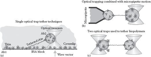
Appropriate latex or silica-based microspheres suitable for optical trapping can be commercially engineered to include a chemical coating of a variety of different compounds, most importantly carboxyl, amino, and aldehyde groups that can be used as adapter molecules to conjugate to biomolecules. Using standard bulk conjugation chemistry, these chemical groups on the bead surface can be bound either directly to biomolecules or more commonly linked to an adapter molecule such as a specific antibody or a biotin group that will then bind to a specific region of a biomolecule of interest (see Chapter 7). Chemically functionalizing microspheres in this way allows single biomolecules to be attached to the surface of an optically trapped bead and tethered to a fixed surface such as a microscope coverslip (Figure 6.3a).
FIGURE 6.3 Tethering single biopolymers using optical tweezers. (a) A biopolymer, exemplified here by the giant molecule title found in muscle tissue, can be tethered between a microscope coverslip surface and an optically trapped bead using specific antibodies (Ab1 and Ab2). (b) A biopolymer tethered may also be formed between an optically trapped bead and another bead secured by suction from a micropipette. (c) Two optically trapped beads can also be used to generate a single-molecule biopolymer tether, enabling precise mechanical stretch experiments.
Several of the first optical tweezers experiments involved the large muscle protein titin (Tskhovrebova et al., 1997), which enabled the mechanical elasticity of single titin molecules to be probed as a function of its molecular extension by laterally displacing the microscope stage to stretch the molecule relative to the trapped bead. This technique was further modified to tether a single titin molecule between an optically trapped bead and a micropipette, which secured to a second bead attached to the other end of the molecule by suction forces (Figure 6.3b), which offered some improvement in fixing the tether axis to be parallel to the lateral plane of movement of the trap thus making the most out of the lateral trapping force available (Kellermayer et al., 1997).
This method was also employed to measure the mechanical properties of single DNA molecules (Smith, 1996), which enabled estimation of the persistence length of DNA of ~50 nm based on wormlike chain modeling (see Chapter 8) as well as enabling observations of phenomena such as the overstretch transition in which the stiffness of DNA suddenly drops at forces in the range 60–70 pN due to structural changes to the DNA helix. Similarly, optical tweezers have been used to measure the force dependence of folding and unfolding of model structural motifs, such as the RNA hairpin (see Chapter 2, and Liphardt et al., 2001). These techniques quantify the refolding of a molecule, indicating that they are far from a simple reversal of the unfolding mechanism (see Sali et al., 1994).
Tethering a single biomolecule between two independent optically trapped beads (Figure 6.3c), offers further advantages of fast feedback experiments to clamp both the molecular force, and position while monitoring the displacements of two separate beads at the same time (Leake et al., 2004). Typically, a single-molecule tether is formed by tapping two optically trapped beads together, one chemically conjugated to one end of the molecule, while the other is coated with chemical groups that will bind to the other end. The two optically trapped beads are tapped together and then pulled apart over several cycles at a frequency of a few Hz. There is however a probability that the number of molecules tethered between the two beads is >1. If the probability of a given tether forming is independent of the time, then this process can be modeled as a Poisson distribution, such that probability Pteth(n) for forming n tethers is given by with the average number of observed tethers formed between two beads (see Worked Case Example 6.1).
The measurement of the displacement of a trapped bead relative to the center of the optical trap allows the axial force experienced by a tethered molecule to be determined from knowledge of the optical tweezers stiffness. The relationship between the force and the end-to-end extension of the molecule can then be experimentally investigated. In general, the main contribution to this force is entropic in origin, which can be modeled using a variety of polymer physics formulations to determine parameters such as equivalent chain segment lengths in the molecule, discussed in Chapter 8.
Several single-molecule optical tweezers experiments are performed at relatively low forces of just a few pN, which is relevant to the physiological forces experienced in living cells for a variety of different motor proteins (see Chapter 2). These studies famously have included those of the muscle protein myosin interacting with actin (Finer et al., 1994), the kinesin protein involved in cell division (Svoboda et al., 1993), as well as a variety of proteins that use DNA as a track. The state of the art in optical tweezers involves replacing the air between the optics of a bespoke optical tweezers setup with helium to minimize noise effects due to the temperature-dependent refraction of lasers through gases, which has enabled the transcription of single-nucleotide base pairs on a single-molecule DNA template by a single molecule of the ribonucleic acid polymerase motor protein enzyme to be monitored directly (Abbondanzieri et al., 2005).
6.3.5 NON-GAUSSIAN BEAM OPTICAL TWEEZERS
“Standard” optical tweezers are generated from focusing a Gaussian profile laser beam into a sample. However, optical trapping can also be enabled using non-Gaussian profile beams. For example, a Bessel beam may be used. A Bessel beam in principle is diffraction free (Durnin et al., 1987). They have a Gaussian-like central peak intensity of width roughly one wavelength, as with a single-beam gradient force optical trap; however, they have in theory zero divergence parallel to the optic axis. In practice, due to finite sizes of optical components used, there is some remaining small divergence at the ~mrad scale, but this still results in minimal spreading of the intensity pattern over length scales of 1 m or more.
The main advantage for optical trapping with a Bessel beam, a Bessel trap, is that since there is minimal divergence of the intensity profile of the trap with depth into the sample, then this is ideal for generating optical traps far deeper into a sample than permitted with conventional Gaussian profile traps. The Bessel trap profile is also relatively unaffected by small obstacles in the beam path, which would cause significant distortion for standard Gaussian profile traps; a Bessel beam can reconstruct itself around an object provided a proportion of the light waves is able to move past the obstacle. Bessel beams can generate multiple optical traps that are separated by up to several millimeters.
Optical tweezers can also be generated using optical fibers. The numerical aperture of a single-mode fiber is relatively low (~0.1) generating a divergent beam from its tip. Optical trapping can be achieved using a pair of juxtaposed fibers separated by a gap of a few tens of microns (Figure 6.4a). A refractile particle placed in the gap experiences a combination of forward scattering forces and lateral forces from refraction of the two beams. This results in an optical trap, though 10–100 times less stiffness compared to conventional single-beam gradient force traps for a comparable input laser power. Such an arrangement is used to trap relatively large single cells, in a device called the “optical stretcher.”
The refractive index of the inside of a cell is in general heterogeneous, with a mean marginally higher than the water-based solution of the external environment (see Chapter 3). This combined with the fact that cells have a defined compliance results in an optical stretching effect in these optical fiber traps, which has been used to investigate mechanical differences between normal human cells and those that have a marginally different stiffness due to being cancerous (Gück et al., 2005). The main disadvantage with the method is that the laser power required to produce measurable probing of cell stiffness also results in large rises in local temperature at the NIR wavelengths nominally employed—a few tens of °C above room temperature is not atypical—which can result in significant thermal damage to the cell.
It is also possible to generate 2D optical forces using an evanescent field, similar to that discussed for TIRF microscopy (see Chapter 3); however, to trap a particle stably in such a geometry requires an opposing, fixed structure oriented against the direction of the force vector, which is typically a solid surface opposite the surface from which the evanescent field emanates (the light intensity is greater toward the surface generating the evanescent field and so the net radiation pressure is normal to that away from the surface). This has been utilized in the cases of nanofabricated photonic waveguides and at the surface of optical fibers. There is scope to develop these techniques into high-throughput assays, for example, applied in a multiple array format of many optical traps, which could have use in new biosensing assays.
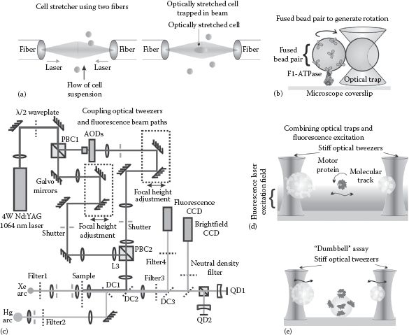
FIGURE 6.4 (See color insert.) More complex optical tweezers applications. (a) Cell stretcher, composed of two juxtaposed optical beams generating a stable optical trap that can optically stretch single cells in suspension. (b) Rotary molecular motors, here shown with the F1-ATPase component of the ATP synthase that is responsible for making ATP in cells (see Chapter 2), can be probed using optical trapping of fused bead pairs. (c) Trapping a fluorescence excitation beam paths can be combined (d) to generate optical traps combined with fluorescence imaging. (e) A 3-bead “dumbbell” assay, consisting of two optically trapped beads and a fixed bead on a surface, can be used to probe the forces and displacements of “power strokes” due to molecular motors on their respective tracks.
6.3.6 CONTROLLING ROTATION USING “OPTICAL SPANNERS”
Cells have, in general, rotational asymmetry and so their angular momentum can be manipulated in an optical stretcher device. However, the trapped particles used in conventional Gaussian profile optical tweezers are usually symmetrical microspheres and so experience zero net angular momentum about the optic axis. Therefore, it is not possible to controllably impart a nonzero mean torque.
There are two practical ways that achieve this using optical tweezers; however, which can both lay claims to being in effect optical spanners. The first method requires introducing an asymmetry into the trapped particle system to generate a lever system. For example, one can controllably fuse two microspheres such that one of the beads is chemically bound to a biomolecule of interest to be manipulated with torque, while the other is trapped using standard Gaussian profile optical tweezers whose position is controllably rotated in a circle centered on the first bead (Figure 6.4b). This provides a wrench-like effect, which has been used for studying the F1-ATPase enzyme (Pilizota et al., 2007). F1 is one of the rotary molecular motors, which, when coupled to the other rotary machine enzyme Fo, generates molecules of the universal biological fuel ATP (see Chapter 2). Fused beads can be generated with reasonable efficiency by increasing the ionic strength (usually by adding more sodium chloride to the solution) of the aqueous bead media to reduce to the Debye length for electrostatic screening (see Chapter 8) with the effect of reducing surface electrostatic repulsion and facilitating hydrophobic forces to stick beads together. This generates a mixed population of bead multimers that can be separated into bead pairs by centrifugation in a viscous solution composed of sucrose such that the bead pairs are manifested as a distinct band where the hydrodynamic, buoyancy, and centripetal forces balance.
The second method utilizes the angular momentum properties of light itself. Laguerre–Gaussian beams are generated from higher-order laser modes above the normal TEM00 Gaussian profile used in conventional optical tweezers, by either optimizing for higher-order lasing oscillation modes from the laser head itself or by applying phase modulation optics in the beam path, typically via an SLM. Combining such asymmetrical laser profiles (Simpson et al., 1996) or Bessel beams with the use of helically polarized light on multiple particles on single birefringent particles that have differential optical polarizations relative to different spatial axes such as certain crystal structures (e.g., calcite particles, see La Porta and Wang, 2004) generates controllable torque that has been used to study interactions of proteins with DNA (Forth et al., 2011).
6.3.7 COMBINING OPTICAL TWEEZERS WITH OTHER BIOPHYSICAL TOOLS
Optical tweezers can be incorporated onto a standard light microscope system, which facilitates combining other single-molecule biophysics techniques that utilize nanoscale sample manipulation and stages and light microscopy–based imaging. The most practicable of these involves single-molecule fluorescence microscopy. To implement optical trapping with simultaneous fluorescence imaging is in principle relatively easy, in that a NIR laser–trapping beam can be combined along a visible light excitation optical path by using a suitable dichroic mirror (Chapter 3), which, for example, will transmit visible light excitation laser beams but reflect NIR, thus allowing the laser-trapping beam to be coupled into the main excitation path of a fluorescence microscope (Figure 6.4c).
This has been used to combine optical tweezers with TIRF to study the unzipping of DNA molecules (Lang et al., 2003) as well as imaging sections of DNA (Gross et al., 2010). A dual optical trap arrangement can also be implemented to study motor proteins by stretching a molecular track between two optically trapped microspheres while simultaneously monitoring using fluorescence microscopy (Figure 6.4d), including DNA motor proteins. Such an arrangement is similar to the DNA curtains approach, but with the advantage that both motor protein motion and molecular force may be monitored simultaneously by monitoring the displacement fluctuations of the trapped microspheres. Lifting the molecular track from the microscope coverslip eradicates potential surface effects that could impede the motion of the motor protein.
A similar technique is the dumbbell assay (Figure 6.4e), originally designed to study motor protein interactions between the muscle proteins myosin and actin (Finer et al., 1994), but since utilized to study several different motor proteins including kinesin and DNA motor complexes. Here, the molecular track is again tethered between two optically trapped microspheres but is lowered onto a third surface-bound microsphere coated in motor protein molecules, which results in stochastic power stoke interactions, which may be measured by monitoring the displacement fluctuations of the trapped microspheres. Combining this approach with fluorescence imaging such as TIRF generates data for the position of the molecular track at the same time, resulting in a very definitive assay.
Another less widely applied combinatorial technique approach has involved using optical tweezers to provide a restoring force to electro-translocation experiments of single biopolymers to controllably slow down the biopolymer as it translocates down an electric potential gradient through a nanopore, in order to improve the effective spatial resolution of ion-flux measurements, for example, to determine the base sequence in DNA molecule constructs (Schneider et al., 2010). There have been attempts at combining optical tweezers with AFM imaging discussed later in this chapter, for example, to attempt to stretch a single-molecule tether between two optically trapped beads while simultaneously imaging the tether using AFM; however, the vertical fluctuations in stretched molecules due to the relatively low vertical trap stiffness have to date been high enough to limit the practical application of such approaches.
Optical tweezers Raman spectroscopy, also known as laser tweezers Raman spectroscopy, integrates optical tweezers with confocal Raman spectroscopy. It facilitates manipulation of single biological particles in solution with their subsequent biochemical analysis. The technique is still emerging, but been tested on the optical trapping of single living cells, including red and white blood cells. It shows diagnostic potential at discriminating between cancerous and non-cancerous cells.
6.3.8 OPTICAL MICROSCOPY AND SCATTERING METHODS TO MEASURE BIOLOGICAL FORCES
Some light microscopy and scattering techniques have particular utility in investigating forces in cellular material. Polarization microscopy (see Chapter 3) has valuable applications for measuring the orientation and magnitude of forces experienced in tissues, and how these vary with mechanical strain. The usual reporters for these mechanical changes are birefringent protein fibers in either connective tissue or the cytoskeleton. In particular, collagen fibrils form an anisotropic network in cartilage and bone tissue, which has several important mechanical functions, largely responsible for tensile and shear stiffness. This method has an advantage of being label-free and thus having greater physiological relevance. The resulting anisotropy images represent a tissue force map and can be used to monitor damage and repair mechanisms of collagen during tissue stress resulting from disease.
FRET (see Chapter 4) can also be utilized to monitor mechanical forces in cells. Several synthetic molecular probes have been developed, which undergo a distinct bimodal conformational change in response to local changes in mechanical tension, making a transition from a compact, folded state at low force to an unfolded open conformation at high force (de Souza, 2014). This transition can be monitored using a pair of FRET dyes conjugated to the synthetic construct such that in the compact state the donor and acceptor molecules are close (typically separated by ~1 nm or less) and so undergo measurable FRET, whereas in the open state the FRET dyes are separated by a greater distance (typically >5 nm) and so exhibit limited FRET. Live-cell smFRET has been used in the form of mechanical force detection across the cell membrane (Stabley et al., 2011). Here, a specially designed probe can be placed in the cell membrane such that a red Alexa647 dye molecule and a FRET acceptor molecule, which acts as a quencher to the donor at short distances, are separated by a short extensible linker made from the polymer polyethylene glycol (PEG). Local mechanical deformation of the cell membrane results in extension of the PEG linker, which therefore has a dequenching effect. With suitable calibration, this phenomenon can be used to measure local mechanical forces across the cell membrane.
The forward and reverse transition probabilities between these states are dependent on rates of mechanical stretch (see Chapter 8). By generating images of FRET efficiency of a cell undergoing mechanical transitions, local cellular stresses can be mapped out with video-rate sampling resolution with a localization precision of a few tens of nm. The technique was first utilized for measurement of mechanical forces at cell membranes and the adhesion interfaces between cells; however, since FRET force sensors can be genetically encoded in much the same way as fluorescent proteins (for a fuller description of genetic encoding technology see Chapter 7), this technique is now being applied to monitoring internal in vivo forces inside cells. Variants of FRET force sensors have also been developed to measure the forces involved in molecular crowding in cells.
Finally, Brillouin light scattering in transparent biological tissue results from coupling between propagated light and acoustic phonons (see Chapter 4). The extent of this inelastic scattering relates to the biomechanical properties of the tissue. Propagating acoustic phonons in a sample result in expansion and contraction, generating periodic variation in density. For an optically transparent material, this may result in spatial variation of refractive index, allowing energetic coupling between the propagating light in the medium and the medium’s acoustic vibration modes.
This is manifested as both an upshift (Stokes) and downshift (anti-Stokes) in photon frequency, as a function of frequency, similar to Raman spectroscopy (Chapter 4), resulting in a characteristic Brillouin doublet on the absorption spectrum whose separation is a metric of the sample’s mechanical stiffness. The typical shift in photon energy is only a factor of ~10−5 due to the relatively low energy of acoustic vibration modes, resulting in GHz level frequency shifts for incident visible light photons. This technique has been combined with confocal scanning to generate spatially resolved data for the stiffness of extracted transparent components in the human eye, such as the cornea and the lens (Scarcelli and Yun, 2007), and to investigate biomechanical changes to eye tissue as a function of tissue age (Bailey et al., 2010) and has advantages of conventional methods of probing sample stiffness in being minimally perturbative to the sample since it is a noncontact and nondestructive technique, without requiring special sample preparation such as labeling.
KEY BIOLOGICAL APPLICATIONS: OPTICAL FORCE TOOLS
Measuring molecular and cellular viscoelasticity; Quantifying biological torque; Cellular separations.
Worked Case Example 6.1 Optical Tweezers
Two identical single-beam gradient force optical tweezers were generated for use in a single-molecule mechanical stretch experiment on the muscle protein titin using an incident laser beam of 375 mW power and wavelength 1047 nm, which was time-shared equally to form two optical traps using an AOD of power efficiency 80%, prior to focusing each optical tweezers into the sample, with each trapping a latex bead of diameter 0.89 μm in water at room temperature. One of the optically trapped beads was found to exert a lateral force of 20 pN when the bead was displaced 200 nm from its trap center.
(a) Estimate the average angle of deviation of laser photons in that optical trap, assuming that the lateral force arises principally from photons traveling close to the optical axis. At what frequency for the position fluctuations in the focal plane is the power spectral density half of its maximum value? (Assume that the viscosity of water at room temperature is ~0.001 Pa · s.)
The bead in this trap was coated in titin, bound at the C-terminus of the molecule, while the bead in the other optical trap was coated by an antibody that would bind to the molecule’s N-terminus. The two beads were tapped together to try to generate a single-molecule titin tether between them.
(b) If one tether binding event was observed on average once in every ntap tap cycles, what is the probability of not binding a tethered molecule between the beads?
(c) By equating the answer to (b) to Pteth(n = 0) where Pteth(n) is the probability of forming n tethers between two beads, derive an expression for in terms of ntap.
We can write the fraction a of “multiple tether” binding events out of all binding events as Pteth(>1)/(Pteth(1) + Pteth(>1)).
(d) Use this to derive an expression for α in terms of .
(e) If the bead pair are tapped against each other at a frequency of 1 Hz and the incubation conditions have been adjusted to ensure a low molecular surface density for titin on the beads such that no more than 0.1% of binding events are due to multiple tethers, how long on average would you have to wait before observing the first tether formed between two tapping beads? (This question is good at illustrating how tedious some single-molecule experiments can sometimes be!)
Answers
(a) Since there is an 80% power loss propagating through the AOD and the laser beam is then time-shared equally between two optical traps, the power in each trap is
Using Equation 6.3, the angle of deviation can be estimated as
Modeling the power spectrum of the bead’s lateral position as a Lorentzian function indicates that the power will be at its maximum at a frequency of zero, therefore at half its maximum . Thus, v = v0, the corner frequency, also given by k/2πγ. The optical trap stiffness k is given by
The viscous drag γ on a bead of radius r in water of viscosity η is given by 6πrη; thus, the corner frequency of the optical trap is given by
(b) The probability of not forming a tether is simply equal to (1 − 1/ntap).
(c) Using the Poisson model for tether formation between tapping beads, the probability Pteth(n) for forming n tethers is given by , thus at n = 0,
Thus,
(d) Fraction of binding events in which >1 tether is formed:
(e) No more than 0.1% tethers due to multiple tether events implies 1 in 103 or less multiple tethers. At this threshold value, a = 0.001, indicating (after, e.g., plotting the dependence of a on ntap from [d] and interpolating) ntap ~ 600 cycles. At 1 Hz, this is equivalent to ~600 s, or ~10 min for a tether to be formed on average.
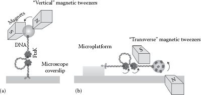
Magnetism has already been discussed as a useful force in biophysical investigations in the context of structural biology determination in NMR spectroscopy as well as for the generation of x-rays in cyclotrons and synchrotrons for probing biological matter (Chapter 5). But magnetic forces can also be utilized to identify different biomolecules from a mixed sample and to isolate and purify them, from using magnetic beads bound to biological material to separate different molecular and cellular components, or from using a magnetic field to deflect electrically charged fragments of biomolecules with the workhorse analytical technique of biophysics, which is mass spectrometry. Also, magnetic fields can be manipulated to generate exquisitely stable magnetic tweezers. Magnetic tweezers can trap a suitable magnetic particle, imposing both force and torque, which can be used to investigate the mechanical properties of single biomolecules if tethered to the magnetic particle.
6.4.1 MAGNETIC BEAD–MEDIATED PURIFICATION METHODS
Magnetic beads are typically manufactured using a latex matrix embedded with iron oxide nanoscale particulates, or other similar ferromagnetic materials such as chromium dioxide. If the concentration of ferromagnetic material in a bead is sufficiently small, then in the absence of an external B-field such beads possess no net magnetic moment. In the presence of an external B-field, the whole resultant bead is magnetized by induction of a magnetic moment aligned with the B-field, but which is lost once the external B-field is removed. This is a property of paramagnetic materials, distinct from ferromagnetic materials, which can retain a net magnetic moment after removing the external B-field. This is a particularly useful feature of beads used for biological purification/isolation methods, since removal of an imposed B-field can then permit separation of components after being isolated from a mixture using a magnetic field. Beads can be chemically functionalized on their surface, using the same technology as for microspheres used for optical tweezers, to permit conjugation to a variety of different biomolecules, such as antibodies and short specific sequences of nucleic acid (see Chapter 7). A suspension of magnetic beads is mixed with the target biological components.
Once bound to a specific biomolecule, then an applied magnetic field can pull the bead, and the biomolecule and any other biological structures attached to that biomolecule (e.g., a whole cell, in the case of the biomolecule attached to a cell membrane receptor protein) away from a mix of heterogeneous biological components/cells, and any unbound material can be removed by aspiration/washing, facilitating purification of that bound component. Magnetic bead–mediated separations result in comparatively low mechanical stress to the biological components being isolated and are rapid, cheap, and high throughput.
Applications include purification of nucleic acids by using short nucleotide sequences (or oligonucleotides, sometimes known simply as oligos) bound to the paramagnetic beads, which are complementary to sequences in the specific target nucleic acid molecules. When coated with specific antibodies, magnetic beads can also be used to purify proteins and to isolate various specific cell types including eukaryotes such as human cells and bacteria, and also smaller subcellular structures and viruses, subcellular organelles, and individual proteins.
For a bulk ensemble average in vitro biophysical technique, mass spectrometry (often shorted to mass spec) is one of the most quantitatively robust. Here, ~10−15 kg of sample (small, but still equivalent to several millions of molecules) is injected into an ionizer. Ionization generates fragments of molecules with different mass and charge. The simplest machine is the sector mass spectrometer that accelerates ion fragments in a vacuum using an electric field E and deflects them using a magnetic field sector oriented at right angles of magnitude B to this so that the ions follow a roughly circular path. The circle radius r is a function of the mass-to-charge ratio mq of particles in the beam, which can easily be derived by equating the magnetic to the centripetal force:
(6.12) |
Different ionized molecule fragments are collected and analyzed depending upon the detector position (often termed a velocity selector) in the circular ion path. This generates a mass spectrum that can yield detailed data concerning the relative proportions of different ionic species in the sample.
Variants of the basic mass spectrometer include ion trap (injected ions trapped in a cavity using electric fields), Fourier transform (ions injected into a cyclotron cell and resonated into orbit using an oscillating electric field generating a radio frequency signal that is detected and subsequently Fourier transformed to yield mass spectrum), time of flight (an ion vapor pulse is created using a high-energy laser and high-energy ions are accelerated using an electric field with time taken to travel a given distance measured), and quadrupole (accelerated ion beam passed between four metal rods to which direct current (DC) and alternating current (AC) potentials are applied causing resonance to the ion beam such that only ions with a narrow range of mq will pass through the rod cavity into the detector unit) mass spectrometers.
The state of the art for quantitative mass spectrometry includes matrix-assisted laser desorption ionization (MALDI, also known as MALDI imaging spectroscopy) and stable isotopic labeling by amino acids in cell culture (SILAC) techniques. MALDI is an imaging technique in which the sample, typically a thin section of biological tissue (which can be applied both to animal and plant tissues), raster scans in 2D while the mass spectrum is recorded, using focused laser ablation of the biological material to generate ion fragments. To enhance laser adsorption, a strongly laser-absorbing chemical reagent matrix is normally sprayed onto the sample surface. MALDI can enable the imaging of the localization of several different biomolecule types including proteins/peptides, lipids, and several other small molecules such as synthetic drugs.
SILAC is a popular technique used in quantitative proteomics, in detecting differences in protein amounts from cell samples using nonradioactive isotope labeling. Typically, two populations of cells are grown in culture medium, one contains normal amino acids, while the other contains amino acids labeled with stable nonradioactive heavy isotopes, usually replacing the normal carbon 12C isotope with the heavier 13C with one more labeled amino acid type in the growth medium. For example, if arginine (which contains six carbon atoms per molecule) was used, then all peptides and proteins containing arginine in the cells would be ~6 Da heavier per molecule of arginine present, compared to the “normal” cell population grown in parallel. Another approach involves more uniform labeling with 13C or the heavier 15N isotope of nitrogen. Both cell populations are then analyzed using mass spectrometry and then compared in a pairwise fashion for chemically identical peptide ion fragments. The measured ratio of signal intensity of such paired fragments in the mass spectrum is an estimate for the relative abundance of a cellular protein that contains those specific heavier amino acids. It can thus be used as a tool to measure the different expression levels of different proteins from a live-cell population.
Biophysical applications of mass spectrometry are significant and include sensitive biological particle detection. The detection sensitivity is around one particle per liter, which compares favorably relative to other bulk ensemble average techniques. A particle can be detected with a sampling time resolution of a few minutes. The technique has been applied for investigations of sample purity quality control, detection of relatively subtle mutations in nucleic acids, protein conformation and folding studies, and proteomics experiments investigating protein–protein interactions. The Simple Analysis at Mars (SAM) instrument suite of NASA’s rover that landed on Mars on August 5, 2012 included a portable mass spectrometer device for detection of putative biological material. Also, the spatial resolution of state-of-the-art mass spec devices now permit precision down to the level of just a few cells and, in some exceptional cases of relatively large cells, just a single cell.
Magnetic particles that have a length scale range of hundreds to thousands of nanometers can be controlled directly and efficiently via the manipulation of the local external B-field, using field strengths in the milli-Tesla (mT) range. This force transduction device is commonly referred to as magnetic tweezers. Both paramagnetic and ferromagnetic beads of around a micron diameter are typical probes used. This has been used to great success for investigating the mechanical properties of several types of biopolymer molecules, especially DNA (Manosas et al., 2010).
The external B-field in the magnetic tweezers setup is usually built as a module to an inverted optical microscope, with either two permanent bar magnets mounted to have juxtaposed poles or a combination of multiple electromagnetic coils to generate a suitable mT B-field placed around the magnetic probe (Figure 6.5a). By moving the microscope stage a candidate bead can be captured in the locally generated B-field. Ferromagnetic beads contain a permanent magnetic dipole moment m, and the interaction between this and the local B-field, as indicated by the gradient of their dot product, results in a force F on the bead and a torque τ, which results from their cross product, rotating the bead in a direction so as to align the magnetic moment with the B-field:
(6.13) |
(6.14) |
It is more common to use paramagnetic beads in magnetic tweezers. In this instance, a magnetic dipole moment is induced in the bead by the external B-field, and in typical ~mT field strengths the magnetization M (given by m/V where V is the bead volume) saturates at a value Mmax. For the most common permanent magnet pair arrangement, the B-field is parallel to the focal plane of the microscope in between the opposite magnet poles, which means that the B-field gradient is zero everywhere apart from the vector normal to the focal plane. Thus, the magnetic force is parallel to optic axis (z) in a direction away from the microscope coverslip surface:
(6.15) |
Thus, a biopolymer tethered between the coverslip and a magnetic bead will be stretched vertically until balanced by the opposing molecular force that increases with molecular extension.
FIGURE 6.5 Magnetic tweezers. Single-molecule mechanical experiments can be performed in both (a) vertical and (b) transverse geometries, for example, to probe the mechanical properties of DNA molecules and of machines, such as FtsK shown here, which translocate on DNA.
The trapped bead’s position is still free to fluctuate in the lateral plane. Considering displacements parallel to the focal plane, the small angle δθ satisfies
(6.16) |
where
z is the molecular extension of the biopolymer parallel to the optic axis
x is the displacement from the equilibrium in the focal plane
The equipartition theorem can be applied similarly as for optical tweezers to estimate the stretching force parallel to the optic axis:
(6.17) |
Measurement of x can be achieved using similar techniques to optical tweezers bead detection, including bright-field detection of the bead image onto a QPD or CCD, or to use BFP detection that is less common for magnetic tweezers systems since it requires an additional focused detection laser to be coaligned with the magnetic trap. As the bead moves above and below the focal plane, its image on a CCD camera contains multiple diffraction rings. The diameter of these rings is a metric for z, which can be determined by precalibration. Measuring the torque on a tethered molecule requires knowledge not only of the magnetic dipole moment and the local magnetic field strength but also the angle between their two vectors. However, since a magnetic bead is spherically symmetrical, this can be difficult to determine unless asymmetry is added, for example, in the form of a marker on the bead for angle of rotation, such as a fluorescent quantum dot (see Chapter 3) fused to the magnetic bead.
The B-field vector can be rotated either by differential phasing of the AC current input through each different electromagnetic coil or by mechanically rotating the two permanent magnets, which thus results in rotation of the magnetic bead. A paramagnetic bead may be similarly rotated by first inducing a magnetic moment in the bead by the presence of a separate nearby permanent magnet.
Usually, the magnetic bead is conjugated to a single biomolecule of interest, which in turn is tethered via its opposite end to a microscope slide or coverslip. By moving the stage vertically relative to the permanent magnets or coils, for example, by changing the focus, the molecule’s end-to-end extension can be controllably adjusted. Therefore, the mechanical properties of individual molecules can be probed with this approach in much the same way as for optical tweezers. One advantage of magnetic tweezers over optical tweezers is that there is potentially less damage to the biological sample, since high stiffness optical tweezers at least require a few hundred mW of NIR laser power, which is sufficient to raise the sample temperature and induce phototoxic effects.
However, a particular advantage of magnetic tweezers is that their relatively easy ability to rotate a particle, in the form of a magnetic bead, compared to technically less trivial optical rotation methods, which enables controllable torque to be applied to a single biomolecule tethered to bead provided appropriate torsional constraints that are inserted into the links between the tether and slide and tether and bead (in practice these are just multiple repeats of the chemical conjugation groups at either end of the biomolecule). This is a more direct and technically simpler method than can be achieved for optical tweezers, which would need either to utilize an extended optical handle or use the rotating polarization of a non-Gaussian mode laser.
Magnetic tweezers–mediated torque control has been used on DNA–protein complexes, for example, to study DNA replication. DNA in living cells is normally a negative supercoiled structure (see Chapter 2), with the supercoiling moderated by topoisomerase enzymes. However, to undergo replication or repair, or to express peptides and proteins from the genes, this supercoiled structure needs first to relax into an uncoiled conformation. To access the individual strands of the double helix then requires this helical structure itself to be unwound, which in turn is made possible by enzymes called helicases. It is likely that many of these torque-generating molecular machines work in a highly coordinated fashion.
A disadvantage of magnetic tweezers over optical tweezers is that they are slower by a factor of ~103 since they do not utilize fast AOD components as optical tweezers can and traditionally require using relatively large micron-sized beads to have a sufficiently large magnetic moment but with the caveat of a relatively large frictional drag, which ultimately limits how fast they can respond to changes in external B-field—a typical bandwidth for magnetic tweezers is ~1 kHz, so they are limited to detect changes over time scales >1 ms. Also, traditionally, it has not been possible to visualize a molecule that has been stretched through application of magnetic tweezers at the same time as monitoring its extension and force, for example, using fluorescence microscopy if the biomolecule in question can be tagged with a suitable dye. This is because the geometry of conventional magnetic tweezers is such that the stretched molecule is aligned parallel to the optic axis of the microscope and so cannot be visualized extended in the lateral focal plane. To solve this problem, some groups are developing transverse magnetic tweezers systems (Figure 6.5b). The main technical issue with doing so is that there is often very confined space in the microscope stage region around a sample to physically position magnets or coils in the same lateral plane as the microscope slide. One way around this problem is to use very small electromagnetic coils, potentially microfabricated, integrated into a bespoke flow cell.
Other recent improvements have involved using magnetic probes with a much higher magnetic moment, which may allow for reductions in the size of the probe, thus incurring less viscous drag, with consequent improvements to maximum sampling speeds. One such probe uses a permalloy of nickel and chromium manufactured into a disk as small as ~100 nm diameter (Kim et al., 2009) and still have a sufficiently high magnetic moment to permit torque experiments in principle on biomolecules such as DNA, which would thus enable faster molecular rotation experiments to be performed.
KEY BIOLOGICAL APPLICATIONS: MAGNETIC FORCE TOOLS
Quantifying biological torque; Molecular and cellular separation and identification; Measuring biomolecular mechanics.
6.5 SCANNING PROBE MICROSCOPY AND FORCE SPECTROSCOPY
SPM includes several techniques that render topographic information of a sample’s surface. There are in excess of 20 different types of SPM that have been developed that can measure a variety of different physical parameters through detection of forces as the probe is placed in proximity to a sample surface, and the variation of these physical parameters across the surface are measured by scanning the probe laterally across the sample. Scanning near-field optical microscopy is one such technique that was discussed previously in Chapter 4. However, the most useful SPM technique in terms of obtaining information on biological samples is AFM. AFM can be utilized both as an imaging tool, but also as a probe to measure mechanical properties of biological matter including cell walls and membranes and, especially, single biomolecules. But there are also a range of other SPM techniques such as scanning tunneling microscopy (STM) and surface ion conductance microscopy (SICM), which have biological applications.
6.5.1 PRINCIPLES OF AFM IMAGING
AFM imaging (Binnig et al., 1986), sometimes known as scanning force microscopy, is the most frequently used SPM technique. AFM had been applied to imaging-purified biomolecule samples conjugated to flat surfaces such as mica, as well as cells. It has also been used to image the topographic surface features of some native living tissues also, for example, blood vessels (see Mao, 2009). This technique shows some promise for in vivo imaging, though the challenge mainly lies in the relatively slow lateral scanning of the sample resulting in problems of sample drift due to the large areas of tissue, which might move before the scan probe can image their extent fully. This is why AFM imaging of biological matter has experienced more successful developments when applied to single cells and purified molecular components.
In AFM imaging, a small, solid-state probe tip is scanned across the surface of the sample (Figure 6.6a), using piezoelectric technology, to generate topographical information. The tip is usually manufactured from either silicon or more commonly the ceramic insulator silicon nitride, Si3N4, with a typical pyramidal or tetrahedral shape of a few microns to tens of microns edge length and height scale. However, a standard AFM tip has a radius of curvature of ~10 nm, which is primarily what determines the spatial resolution, though in some specially sharpened tips this can be an order of magnitude smaller.
FIGURE 6.6 Atomic force microscopy imaging. (a) Samples are raster scanned laterally relative to an AFM tip, such that the cantilever on the tip will deflect due to topographical features, which can be measured by the deflection of a laser beam. (b) Schematic for the Hertz model of biological material deformation. (c) Standard AFM cantilever size and shape. (d) Shape of energy potential curve for a tip–cantilever system as a function of the tip–sample distance.
The AFM tip is attached to a cantilever, which is normally manufactured from the same continuous piece of material (a Si-based wafer) via photolithography/masking/wet etching (see Chapter 7). The silicon or silicon nitride cantilever may be subsequently coated with a metal on the “topside,” which can be used to enhance laser reflection for positional detection (see in the following text). The cantilever acts as a force actuator, with the tip detecting a superposition of several different types of forces between it and the sample, both attractive and repulsive, which operate over long lengths scales in excess of 100 nm from the surface through to intermediate and much shorter length scale forces over distances of just a single atom of ~0.1 nm. The thin, flexible metallic cantilever strip is ~0.1 mm wide and a few tenths of a mm long, and as the tip approaches the surface repulsive forces dominate and cause the metallic strip to bend upward. In essence, this bending of cantilever gives a readout of distance between the tip and the sample, which allows the surface topography to be mapped out.
6.5.2 FORCES EXPERIENCED DURING AFM IMAGING
The tip–sample interaction can be described as the total potential energy Utotal, which is the sum of three potentials USD (which is due to the sample deformation as the tip approaches), UME (which is due to the mechanical elastic potential of the cantilever bending), and UIP (which is the interaction potential between the sample and the tip), resulting in the total force F on the AFM tip:
(6.18) |
Sample deformation forces are not trivial to characterize due to the often heterogeneous and nonlinear elastic response of soft matter. The Hertz model offers a reasonable approximation however for a small local sample indentation zS such that the restoring force FSD (see Figure 6.6b) is given by
(6.19) |
where Rtip is the radius of curvature of the AFM tip being pushed toward a sample of Young’s modulus Ysample, with the Poisson ratio of the soft-matter material given by μ.
The restoring mechanical force resulting from deflections of the cantilever is easier to characterize since it can be modeled as a simple Hookean spring, such that FME = −kzz where kz is the cantilever’s vertical stiffness and z is the small vertical displacement of the cantilever from its equilibrium zero force position. Thus, this mechanical elastic potential has a simple parabolic shape. Whereas the local stiffness of the sample is often difficult to determine directly, the well-defined geometry and mechanical properties of the cantilever enable a more accurate estimation of its stiffness to be made.
For standard mode force sensing, the AFM cantilever oscillations can be approximated as those of a solid beam flexing about its point of attachment, namely, that of a beam-like structure that has one relatively compliant axis (normal to the cantilever flat surface) in terms of mechanical stiffness, with the two remaining orthogonal axes having comparatively high stiffness values. The beam bending equation of classical mechanics, for which one end of the beam is fixed while the other is allowed to undergo deflections, can be used to estimate the bending stiffness parallel to the z-axis, kz as
(6.20) |
where
wi is the width of the cantilever beam parallel to the ith axis (Figure 6.6c)
Y is the Young’s modulus
This beam–cantilever system also has a resonance frequency ν0 given by
(6.21) |
where
m0 is the effective total mass of the cantilever and AFM tip
ρ is the cantilever density
Measurement of the resonance frequency far from the surface (such that the potential energy function is dominated solely by the mechanical elasticity of the cantilever with negligible contributions from surface-related forces) can be used to estimate kz. However, this relies on accurate knowledge of the material properties of the cantilever, which are often not easy to obtain due to the variability from cantilever to cantilever in a given manufactured batch.
An alternative method involves measuring the vertical mean squared displacement far away from the sample surface, which requires only an accurate method of measuring z. Deflections of the cantilever can be very accurately detected usually involving focusing a laser onto the reflecting back of the polished metal cantilever and imaging the reflected image onto a split photodiode detector. The voltage response is converted ultimately to a corresponding distance displacement of the tip, provided that the cantilever stiffness has been determined.
We can then use the equipartition theorem in a similar way as for quantifying the stiffness of optical and magnetic tweezers to estimate . At a room temperature of ~20°C, kBT is ~4.1 pN⋅nm (see Chapter 2). Thus, if the voltage output V from a photodiode results in a volts per nm of cantilever vertical deflection, the z stiffness is given roughly by 4.1a2/〈V2〉 in units of pN/nm. Typical cantilever stiffness values used for probing biological material in AFM are ~0.1 pN/nm (see Worked Case Example 6.2).
The interaction forces experienced by the tip include electrostatic and chemical forces as well as van der Waals (vdW) forces. The Morse potential is a good qualitative model for the chemical potential, in characterizing to the potential energy due to the separation, z, of two atoms that can form a chemical bond to create a diatomic molecule when they approach each other to within ~0.1 nm, as might occur between atoms of the sample and the approaching tip. The shape of the potential energy curve has a minimum corresponding to the equilibrium atom separation, σ, which is ~0.2 nm, so the term potential energy well is appropriate. The functional form of the Morse potential is
(6.22) |
where Ebond is the bonding energy, with a decay length κ. Quantum mechanics can predict an exact potential energy curve for the H2+ diatomic molecule system, which the Morse potential fits very well, whose form exhibits the qualitative features at least of the real AFM chemical potential energy function. However, for more complex chemical interactions of higher atomic number atoms involving anisotropic molecular orbital effects, as occurred in practice with the tip–sample system for AFM, empirical models are used to approximate the chemical potential energy, including the Stillinger–Weber potential and Tersoff potential, with the Stillinger–Weber potential showing most promise from ab initio calculations for interactions involving silicon-based materials (as is the case for AFM tips). The functional form of this potential energy involves contributions from nearest-neighbor and next nearest-neighbor atomic interactions. The nearest-neighbor component UNN is given by
(6.23) |
where A, B, a, p, and q are all constants to be optimized in a heuristic fit. The next nearest-neighbor component, UNNN, is a more complex formulation that embodies angular dependence of the atomic orbitals:
(6.24) |
such that
(6.25) |
where
λ is a constant
i, j, and k are indices for three interacting atoms
If an AFM tip is functionalized to include electrostatic components, these can interact with electrostatic components on the biological sample surface also. The functional form can be approximated as where ε is electrical permittivity of the aqueous solvent surrounding the tip and sample, Rtip is again the AFM tip radius of curvature and V is the electrical potential voltage across a vertical distance z between tip and sample.
The most significant of the interaction forces for AFM are the vdW forces, modeled as the Lennard-Jones potential (also known as the 6–12 potential, introduced in Chapter 2):
(6.26) |
The vdW forces arise from a combination of the fluctuations in the electric dipole moment, and the coupling between these fluctuating dipole moments, and the exclusion effect between paired electrons. The longer-range ~z6 dependence is the attractive component, while the shorter-range ~z12 component results from the Pauli exclusion principle between paired electrons that prohibits electrons with the same spin and energy state from occupying the same position in space and thus results in a repulsive force at very short tip–sample separations. However, approximating the tip as a sphere of radius Rtip and assuming interactions with a planar sample surface, we can integrate the incremental contributions from the sphere using Equation 6.26 to give
(6.27) |
where AH is the Hamaker constant depending on the tip and sample electrical polarizability and density. As Figure 6.6d illustrates, the combination of multiple independent potential energy functions experienced by an AFM tip, which operate over different length scale regimes, results in a highly nonlinear force–distance response curve.
During AFM imaging, the tip–cantilever force actuator can be used either in contact mode, noncontact mode, tapping mode, or a relatively newly developed torsional mode. During contact mode imaging, the cantilever deflection is kept constant throughout as the tip is scanned across the sample surface using fast feedback electronics from the photodiode detector to a piezo actuator controlling the cantilever z position, to maintain a constant force on the tip (and hence constant height above the surface, assuming the material properties of the sample remain the same). Here, although the tip itself does not make direct contact as such with the sample, it is placed in relatively close contact to it (typically less than the equilibrium atom separation of ~0.2 nm) such that the overall force detected by the tip from the sample is in the short-range repulsive force regime.
As Figure 6.6d suggests, the force, as the gradient of the potential energy curves, varies dramatically with vertical displacement, with typical forces being in the range 10−6 to 10−9 N. This high sensitivity to vertical displacement allows potentially atomic-level resolution to be obtained in contact mode. However, shearing forces at short distances from the sample are high potentially resulting in sample distortion, in addition to sample damage from scraping of soft sample features by the AFM tip during lateral scanning.
Although atomic-level resolution in z can in principle be obtained in contact mode, the finite AFM tip radius of curvature results in a limit on the absolute maximum measurable z displacement (i.e., height) between neighboring surface features. If, for example, similar sharp surface features are separated by a characteristic displacement d in the lateral surface plane, then the maximum height Δz, which an AFM tip of radius of curvature Rtip could measure, is given from simple space constraints as
(6.28) |
In contact mode imaging, the AFM tip can penetrate beyond water layers bound to the surface to image the sample molecules directly, manifested in a greater spatial resolution. However, the finite sharpness of the AFM tip itself means that some sample surface features will be inaccessible with a resultant tip broadening convolution artifact (see Worked Case Example 6.2). The AFM tip experiences a lateral force from a stiff object on the surface when the AFM tip is pushed down vertically during imaging. If the half angle of the tip’s triangular cross section is θ, then simple geometrical considerations indicate that the tip broadening coefficient κ, defined as the ratio of the apparent measured width r′ of the stiff object (modeled as a sphere with a circular cross section of radius r), satisfies
(6.29) |
In noncontact mode imaging the AFM tip is kept far from the sample surface often much greater than the equilibrium atom separation of ~0.2 nm such that forces experienced by the tip are in the attractive force regime of the force–displacement response curve. In this regime, the tip can be several nm to tens of nm from the sample surface resulting in much weaker forces compared to contact mode, of ~10−12 N (i.e., ~pN). Noncontact mode imaging therefore has an advantage in minimizing the vertical force on a sample, important in general cases of relatively compliant material, therefore minimizing sample deformation and also minimizing the risk of sample damage from lateral scanning. However, the spatial resolution is poorer compared to contact mode with slower scanning speeds permissible. Also noncontact mode ideally requires hydrophobic samples to minimize the thickness of adsorbed water solvent on the sample, which would otherwise impair the scanning by trapping the tip in the adsorbed layer. If a nonhydrophobic sample is in physiological water-based pH buffer environment (as opposed to a high vacuum as would be the case to generate the lowest measurement of noise), then noncontact mode will in general image not only the sample surface but also the first few shells of water molecules, which reduces the imaging spatial resolution.
In tapping mode imaging, the cantilever is driven to oscillate vertically at a distance of 100–200 nm from the sample surface with an amplitude of at least ~10 nm, with a frequency marginally above its resonance frequency. As the tip approaches the sample surface during its periodic oscillation, the increase in attractive forces results in a decrease of the amplitude of oscillation, with an associated change of phase. Depending upon the measurement system, either the change in frequency can be detected (frequency modulation) or the change in amplitude or phase (amplitude modulation); the latter of which is relatively sensitive to the type of sample material being imaged. These detected signal changes can all be converted after suitable calibration into a distance measurement from the sample. Such AFM imaging has been able to measure several types of single biomolecules (Arkawa et al., 1992), including snapshots of the motor protein myosin during its power stroke cycle, and also, to visualize artificial lipid bilayers containing integrated single protein complexes in a physiological aqueous environment.
A traditional weakness of AFM is the relatively slow imaging speeds due to slow scanning and feedback electronics. Recent improvements have been made in improving the imaging speed, the so-called high-speed AFM, using a combination of sharp AFM tips with a greater natural resonance frequency, or by using torsional mode imaging. Here, the AFM cantilever oscillates through a twisting vibrational mode as opposed to a vertical one. This has resulted in video-rate imaging speeds (Hobbs et al., 2006), which have been employed for measuring actual real-time stepping motions of the key molecular motor molecule of myosin, which is responsible for the contraction of muscle tissue, though the lateral spatial resolution is in principle slightly worse than nontorsional AFM for an equivalent tip due to the additional torsional sweep of the end of the probe.
AFM imaging and scanning electron microscopy (SEM) (see Chapter 5) can both generate topographical data from biological samples. AFM has some advantages to SEM: no special sample staining or elaborate preparation is required and the spatial resolution can be at the nm scale as opposed to tens of nm with SEM. However, there are also disadvantages: AFM has relatively slow scanning speeds for comparable levels of spatial resolution, which can lead to issues of drift in the sample (most usually thermal related drift effects), the scan area for AFM is much smaller than for SEM (usually a few tens of μm squared for AFM, as opposed to several hundred μm squared for SEM), differences between AFM tips and cantilever even in the same manufactured batch can lead to image artifacts as well as there being unavoidable tip broadening artifacts, and also piezoelectric material driving the lateral scanning of the tip and the vertical displacement of the cantilever can suffer cross talk between the x, y, and z axes. Also, AFM can image samples under liquid/physiological conditions with a suitable enclosed cell, whereas SEM cannot. However, the choice of which biophysics technique to choose to render topographic detail should clearly be made on a case-by-case basis.
6.5.4 SINGLE-MOLECULE AFM FORCE SPECTROSCOPY
AFM can also be used to investigate the mechanical elasticity of single biomolecules (Figure 6.7a) in a technique called AFM force spectroscopy. In the simplest form, AFM force spectroscopy experiments involve nonspecific binding of the biomolecule in question to a gold or platinum coated coverslip followed by dipping an AFM tip into the surface solution. Upon then retracting the AFM tip back, there is a probability that a section of a molecule is nonspecifically tethered between the tip, for example, by hydrophobic binding, and the coverslip. In having tethered a section of a single molecule, the tip–cantilever system can then be used to investigate how the molecular restoring force varies with its end-to-end extension, similar to optical and magnetic tweezers discussed previously in this chapter.
FIGURE 6.7 Atomic force microscopy (AFM) molecular manipulation methods. (a) AFM force spectroscopy using a “fishing” approach to tether a peptide construct, consisting of repeat “Ig domain” subunits, which results in (b), a characteristic sawtooth response of the force versus extension relation. (c) An AFM tip can be used to controllably relocate single DNA “cargo” molecules to different regions of a gold-coated coverslip.
Simple AFM force spectroscopy devices can be limited to just one axis of controllable movement for the vertical axis controlled by a piezo actuator to move the AFM tip relative to the sample (these one-axis instruments in effect relying on lateral sample drift to move to a different region of the sample, so there is a paradoxical benefit in having a marginally unstable system). Single-molecule AFM force spectroscopy experiments are often performed on modular proteins, either purified from the native source or using smaller synthetic molecules that allow shorter sections of the native molecules to be probed in a more controllable way than the whole native molecule. The large muscle protein titin, discussed previously in the context of optical tweezers, has proved to be an invaluable model system in AFM force spectroscopy studies. In one of the best examples of such pioneering experiments, single molecule constructs consisting of up to eight repeats of the same protein “Ig” domain (Rief et al., 1997).
The properties of the molecule titin are worth discussing in greater detail due to its importance in force spectroscopy experiments and our subsequent understanding of molecular mechanical properties. Titin is an enormous molecule whose molecular weight lies in the MDa range, consisting of ~30,000 individual amino acid residues and is part of a filamentous system in muscle, which act as springs to align the functional subunits of muscle tissue called sarcomeres. Most of the molecule is composed of repeating units of β-barrel modules of ~100 amino acid residues each, which either belong to a class called “fibronectin (Fn)” or “immunoglobulin (Ig),” with a combined total in excess of 370 combined Fn and Ig domains.
The increased likelihood of unfolding of the β-barrel structure of Fn or Ig domains as force is increased on the titin possibly confers a shock-absorber effect, which ensures that the myofibril, the smallest fully functional filamentous subunit of muscle tissue compared to multiple repeating sarcomeres, can maintain structural integrity even in the presence of anomalously high forces, which could damage the muscle. Titin is made in a variety of different forms with different molecular weights depending on the specific type of muscle tissue and its location in the body, and there is good evidence to indicate that this allows the titin molecular stiffness to be catered to the range of force experienced in a given muscle type.
In fishing for surface-bound titin constructs, a variable number of Ig modules in the range 1–8 can be tethered between the gold surface and the AFM tip depending on the essentially random position of the nonspecific binding to both. These domains unfold in the same manner as those described for mechanical stretch experiments on titin using optical tweezers, with a consequent sudden drop in entropic force from the molecule and increase in molecular extension of ~30 nm, due to an Ig domain making a transition from a folded to an unfolded conformation. Thus, the resultant force-extension relation has a characteristic sawtooth pattern, with the number of “teeth” corresponding to the number of Ig domains unfolded in the stretch, and therefore varying in the range 1–8 in this case (Figure 6.7b). These sawtooth patterns are important since they indicate the presence of a single-molecule tether, as opposed to multiple tethers, which might be anticipated if the surface density of molecules is sufficiently high. The sawtooth pattern thus denotes a molecular signature.
AFM force spectroscopy can also be used with greater binding specificity by chemically functionalizing both the AFM tip and the gold or platinum surface. Many AFM force spectroscopy devices are also used in conjunction with an xy nanostage that allows lateral control of the sample to allow reproducible movements to different sample regions as well as force feedback to clamp the molecular force to a preset value to enable definitive observation of force-dependent kinetics of unfolding and subsequently refolding of molecular domains (details of analytical methods to model these processes are discussed in Chapter 8).
The spatial reproducibility and resolution of many AFM systems is high enough such that single molecules may be pulled clear from a surface, moved laterally by anything from a few nm to several microns, and then controllably repositioned by pressing the tip back into the surface (Figure 6.7c). This in effect is a molecular cut-and-paste device (Kufer et al., 2008). By combining AFM cut and paste with the specificity of DNA base pairing, it has been possible to use a complementary DNA strand conjugated to an AFM tip to specifically capture surface-bound DNA constructs from a “depot” region on the surface of the sample and repositioned elsewhere on the surface, offering future potential for smart designed synthetic biology applications at the nanometer length scale (discussed in Chapter 9).
6.5.6 AFM AND FLUORESCENCE MICROSCOPY
Single-molecule experiments are increasingly characterized by combinatorial approaches—combining simultaneous measurements on the same molecule but using different single-molecule methods. An example of this is the combination of AFM force spectroscopy with fluorescence microscopy (Sarkar et al., 2004). For example, it is possible to engineer constructs that have a single Ig domain bounded by fluorescent protein FRET dye pairs. In the unfolded Ig domain conformation the separation of the FRET pairs is <5 nm and therefore results in a measurable FRET efficiency (see Chapter 4). If the molecule is the stretched using AFM force spectroscopy, then the unfolding of the Ig domain results in an increase in the FRET dye pair separation by ~30 nm, thus resulting in no measurable FRET efficiency between the acceptor and donor pair. This therefore constitutes a “double” molecular signature that gives a significant increase in confidence that one is really observing a single-molecule event. Single-molecule fluorescence imaging has also been utilized in AFM cut-and-paste techniques to confirm the correct placement of repositioned DNA molecules.
6.5.7 AFM TO MEASURE CELLULAR FORCES
An AFM cantilever–tip force actuator can be used as a probe to measure cellular mechanical forces by probing regions of the cell that are accessible to the AFM tip. These include elastic and viscoelastic forces present in the cell membrane and cell wall, as well as the mechanical properties of the cytoskeleton just beneath the cell membrane and forces of adhesive, which are used to stick certain cells together in structural tissues. AFM can be used to generate maps of mechanical properties including the Young’s modulus and stiffness values across the surface of a cell. Often, to avoid damage to the relatively soft cell membrane, an AFM tip can be modified by conjugating a larger “blunter” probe onto the end of the AFM tip, for example, a latex microsphere. Mechanical forces are particularly important in characterizing cancerous cells, since these often change in stiffness compared to noncancerous cell types as well as having reduced cell-to-cell adhesion forces (investigated, e.g., in cells called fibroblasts present in connective tissue), which thus increases their chance of breaking free from a tumor or metastasizing, that is, spreading to other parts of the body. Measurement of mechanical properties at a single-cell level may therefore have future diagnostic potential in biomedicine.
AFM force spectroscopy (as well as optical and magnetic tweezers) suffers similar issues in regard to being applicable to measurements inside the living cells, as opposed to being applied to features that are accessible from the cell surface. Recent developments in synthetic transmembrane adaptor molecules, which can integrate into a cell membrane but bind both to internal cellular substructures and/or molecular complexes and to external molecules on the outside of the cell, may in the near future be functional as suitable “handles” for AFM tip probes (and indeed for trapped microspheres inside the cell) to allow access to monitoring internal cellular force-dependent processes.
A novel variant of AFM that has applications to cellular force measurements and probing is the fluid force microscopy (or FluidAFM). Here, a microfluidics channel (see Chapter 7) is engineered into the cantilever extending down through the AFM tip, which allows the tip end to function as a suction nanopipette. This can be used, for example, to manipulate single cells and/or probe their cell membranes.
6.5.8 SCANNING TUNNELING MICROSCOPY
STM was the seed to all SPM techniques. It was developed in the early 1980s (Binnig et al., 1982) and uses a solid-state scanning probe tip, similar to that used for AFM imaging experiments, but which can conduct electrons away from the surface of an electrically conducting sample in a vacuum environment. Tips are made from gold, platinum/iridium, or tungsten, manufactured usually by chemical etching (though historically a narrow wire could be cut to produce a sharp enough tip). Nonmetallic but electrically conducting carbon nanotubes have also been utilized, which have some advantages of a better manufacturing reproducibility and mechanical stability. Electrical conduction at the tip is mediated through the atom of the tip closest to the sample surface, and so the effective radius of curvature is ~1–2 orders of magnitude smaller than that for AFM tips.
No physical contact is made between tip and sample, and therefore there is a classically forbidden energy gap across which electrons must quantum tunnel across for electrical conduction to occur (Figure 6.8a). In the classical picture, if an electron particle of speed v and charge q has kinetic energy E of ~mv2/2, then it will not be able to travel to a region of space, which involves crossing a potential energy barrier P of qV where V is the electrical potential voltage difference if qV > mv2/2 since this implies an electron with negative kinetic energy in the barrier itself, and so instead the electron is reflected back from the boundary.
However, in a quantum mechanics model the electron particle is also an electron wave, which has a finite probability of tunneling through the potential barrier. This can be demonstrated by solving Schrödinger’s wave equation in the barrier that results in a nonperiodic evanescent wave solution whose transmission coefficient, T, for a rectangular shaped barrier of width z, takes the form
(6.30) |
The tunneling electron current IT depends on the tip–sample separation z and the effective width wxy in the lateral xy plane of the sample over which tunneling can occur as
(6.31) |
where
I0 is the equivalent current at zero gap between the tip and the sample
A is a constant equal to (4π/h)(2m)1/2 where h is Plank’s constant and m the free-electron mass
FIGURE 6.8 Other scanning probe microscopies. (a) Scanning tunneling microscopy and (b) scanning ion conductance microscopy.
The free electron depends upon the electrical potential energy gap between tip and sample, and so A is sometimes written in non-SI units as 1.025 Å eV−1/2. The exponential dependence of IT in terms of tip–sample distance makes it very difficult to measure the current experimentally if the distance is greater than a few tenths of a nanometer from a weakly conducting surface such as a biological sample.
STM is usually operated in a constant current imaging mode, analogous to the constant height or force mode of AFM, that is, IT is kept constant using feedback electronics to vary the height of the tip from the sample, typically using a highly sensitive low-noise piezoelectric device, while the probe is laterally raster scanned. The variation in measured sample height is thus a measure of the sample topography, which can be converted into a 3D contour plot of the sample surface in much the same way as for AFM. A less common mode of operation is for the tip–sample distance z to be kept a constant such that the variation in tunneling current itself can be converted into topographical information. This has the advantage of not requiring electronic feedback, which ultimately can permit faster imaging, though it requires a sample to be, in effect, smooth at the atomic level, and so is of limited use for imaging biological material.
The spatial resolution of STM is less sensitive to the tip’s size and shape as is the case for AFM and is ~0.1 nm laterally (i.e., the length scale of a single atom) and ~0.01 nm vertically. STM therefore provides lateral information at an atomic resolution but topographical data at a subatomic resolution. The main limitation for its use in biology is that most biological matter is only very weakly electrically conducting and so generates small values of IT that are difficult to measure above experimental noise. However, STM has been used to image single DNA molecules, protein complexes made up of large macroglobulin molecules, and single virus particles (Arkawa et al., 1992).
AFM has also been combined with STM and Kelvin probe microscopy. Here, an ultracold probe tip with at a temperature of just ~5 K is used to measure the actual distribution of electronic charge in a single molecule, in this case an organic molecule called naphthalocyanine. This has been used in the context of developing single-molecule logic switches for bionanotechnological purposes (Mohn et al., 2012).
6.5.9 SCANNING ION CONDUCTANCE MICROSCOPY
For scanning ion conductance microscopy (SICM), the probe consists of a glass pipette drawn out such that its end diameter is only ~20–30 nm (Hansma et al., 1989). This technique combines the scanning probe methods of SPM with the ion-flux measurements methods of patch clamping (discussed later in this chapter). An electric potential is applied across the end of the tip, which results in a measureable ion current in physiological ionic solutions. However, as the tip is moved to within its own diameter from the biological sample being scanned, the ion flow is impeded.
Using fast feedback electronics similar to those described previously for AFM and STM, this drop in ion current can be used to maintain a constant distance between the nanopipette tip and the sample. This can generate topographical information as the tip is laterally scanned across the surface (Figure 6.8b). SICM has a poorer spatial resolution compared to STM or AFM of ~50 nm, but with an advantage of causing less sample damage. Recent improvements, primarily in narrowing the diameter of the pipette to ~10 nm, have enabled noncontact imaging of collections of single protein molecular complexes on the outer membrane surface of live cells. Also, SICM has been used in conjugation with single-molecule folding kinetics studies of fluorescent proteins by using the same nanopipette to deliver a denaturant to chemically unfold, and hence photobleach, single fluorescent protein molecules, prior to their refolding and gaining photoactivity (Klenerman et al., 2011).
6.5.10 ULTRASONIC FORCE MICROSCOPY
Ultrasonic force microscopy (UFM) (Kolosov and Yamanaka, 1993), also referred to as atomic force acoustic microscopy and essentially the same as scanning near-field ultrasound holography, applies similar principles of AFM imaging in using a silicon or silicon nitride tip attached to a metallic cantilever, which is scanned laterally across the sample surface. However, in UFM, the sample is coupled to a piezoelectric transducer below the sample and a second transducer to the cantilever, which both emit longitudinal acoustic waves of slightly different frequencies close to the resonance frequency of the tip–cantilever system. These waves are propagated into the sample and then result in an acoustic interference pattern. The acoustic vibrations from the interference pattern are picked up by the tip and transmitted into the cantilever, either through the sample media of air or water or through direct contact with the sample in the case of vacuum imaging. Cantilever oscillations are then detected in the same manner as for AFM using laser beam reflected and imaged onto a split photodiode.
Greatest sensitivity is achieved using force acoustic frequencies slightly higher than the resonance frequency of the normal flexure mode of the tip–cantilever system, usually from ~10 kHz up to ~5 MHz. The perturbations to both phase and amplitude across the sample surface in the acoustic standing wave are locally monitored by the tip, which acts as an acoustic antenna via a lock-in amplifier. Note that there are many common standard forms of instrumentation used in biophysics, which we will not explore in depth of this book; however, the lock-in amplifier is of particular use and is singled out here. It is an electronic amplifier common to many other applications of biophysics that can pull out and amplify a signal from a very specific frequency carrier wave from an otherwise extremely noisy environment, often in cases where the signal amplitude is up to six orders of magnitude smaller than the typical noise amplitude. As such it has myriad uses in single-molecule biophysics signal detection and amplification in particular.
Monitoring perturbations of the AFM tip in this way not only generates topographical information from the sample but also is a direct measure of elastic properties. For example, it can be used to infer the Young’s modulus deeper in the sample in the region directly below the scanned tip, with an effective spatial resolution of 10–100 nm (Shekhawat and Dravid, 2005). Biological applications have included the imaging of malarial parasites buried deep inside red blood cells and monitoring aggregation effects in vitro of amyloid peptides (important precursors of various forms of dementia when misfolded, see Chapter 2).
KEY BIOLOGICAL APPLICATIONS: AFM
Imaging biological surface topography; Measuring molecular viscoelasticity and mechanics.
Worked Case Example 6.2 AFM Imaging
In an AFM imaging experiment, the cantilever–tip system was composed of a tetrahedral-shaped silicon nitride tip of height 10 μm with tip end radius of curvature 15 nm, which was fixed to a cantilever of mass 25 pg, such that the tip was located at the end of the cantilever’s 0.1 mm long axis. The cantilever width was equal to the tetrahedron tip edge length.
(a) What is the value of the cantilever resonance frequency in kHz and its stiffness in units of pN/nm? Comment on how these compare with the stiffness of typical “stiff” optical tweezers.
(b) How does the effective mass of the AFM tip–cantilever system compare with the mass of the cantilever and the mass of the tip?
AFM imaging was performed using this tip–cantilever system in contact mode to investigate an array of spike structures called “pili” (singular = “pilus”) covering the surface of a spherical bacterial cell of ~2 μm diameter. Prior SEM imaging suggested that pili have a mean ~1 μm length and are composed of ~1000 copies of a subunit protein called “PapA,” with pili expressed over the surface uniformly with a surface density that did not depend on the cell size. When the tip was scanned between consecutive pilus spikes, the estimated vertical force on the cantilever dropped by ~20 nN.
(c) If the range of cell diameters in a population is ~1–3 μm, estimate the range in PapA copy numbers per cell, stating assumptions you make.
(d) The estimated mean width of a single pilus from earlier SEM imaging was 2.5 nm; however, AFM imaging suggested a width of almost 5 nm. Explain this discrepancy.
(You may assume that the density and Young’s modules of steel are 8.1 × 10³ kg m−3 and 210 GPa, and the density of silicon nitride is 3.4 × 10³ kg m−3.)
Answers
(a) We can first deduce the dimensions of the cantilever: wx = 0.1 mm, wy is equal to the edge length a of a tetrahedron of height h of 10 μm—tetrahedral trigonometry indicates that wy = a = h(3/2)1/2 = 12.2 μm. The volume V of the cantilever is calculated from mass/density:
Thus,
The resonance frequency equation for a deflecting beam thus indicates
“Stiff” optical tweezers have a typical stiffness of ~0.1 pN/nm, so this AFM cantilever is ~4 orders of magnitude stiffer.
(b) Rearranging the beam equation to give the total effective mass of the cantilever-tip system indicates
which is ~3 times the mass of the cantilever. The volume of the tip is given by the tetrahedron formula of (1/3) × base area × height = 2.1 × 10⁻¹⁶ m3
Thus, the tip mass = (3.4 × 103) × (2.1 × 10−16) = 0.7 pg, which is ~2 orders of magnitude smaller than the effective mass of the cantilever–tip system and thus negligible.
(c) From Hooke’s law, the change in vertical displacement of the cantilever corresponding to a 20 nN drop in force is
Assuming sample deformation effects are negligible, this indicates that the average lateral spacing between pili on the surface is
Model the occupancy area around each pilus as a circle of radius 155/2 = 78 nm. Thus, the mean surface density of pili is
The range of cell diameters in a population is 1–3 μm, equating to an area range of 3.1–28.3 μm2. Thus, the range of number of pili in the population is 161–1450 per cell, 1000 PapA molecules per pilus, and therefore the copy number, assuming all cellular PapA expressed in pili, is 1.6 × 10⁵ to 1.5 × 10⁶ PapA molecules per cell.
(d) The tip broadening artifact results in an apparently larger pilus width. The half angle of tip is ~(180 – 109.5) = 35.3° where 109.5° is the tetrahedral angle, so tip broadening is tan(35.3°) + sec(35.3°) = 1.9, so the apparent width measured by AFM imaging of pilus will be ~2.5 × 1.9 = 4.8 nm, as observed.
Electrical forces can be used to control the mobility of molecules (e.g., in gel electrophoresis) as well as generating stable traps for biological particles (anti-Brownian electrophoretic/electrokinetic traps [ABEL traps]) and controlling their rotation (electrorotation). One of the most important applications of electrical forces is in the measurements of ion fluxes through nanopores. If a small hole is made in a sheet of electrical insulator surrounded by an ionic solution and an electrostatic potential difference applied across the sheet, then ions will flow through the hole. If the hole itself has a length scale of nanometers (i.e., a “nanopore”), then this simple principle can form the basis of several biophysical detection techniques, most especially patch clamping.
Gel electrophoresis is one the of most ubiquitous and routine biophysical techniques in modern biochemical research laboratories, but is still in many ways one of the most useful for its ability to separate the components of a complex in vitro sample composed of a mixture of several different biomolecules in a simple, relatively fast and cheap way, and to characterize these molecules, on their basis of their size, charge, and shape. Usually, a sample of a few tens of microliters in volume is injected into a semiporous gel and exposed to an electric field gradient. The gel is composed of either polyacrylamide (for protein samples) or agarose (for samples containing nucleic acids), with space for ~10 parallel channels in each gel so that different samples can be run under the same conditions simultaneously. Gels are cast with a characteristic concentration that affects the distribution of pore sizes in the gel matrix. Smaller molecules will therefore diffuse faster through this mesh of pores than larger molecules.
Equating the electrical force to the drag force indicates that the drift speed vd of a molecule of net charge q during gel electrophoresis across an electric field E is given by
(6.32) |
Protein samples may either be first denatured by heating and combined with an ionic surfactant molecule such as sodium dodecyl sulfate (SDS), or may be run in a nondenatured native state. SDS disrupts noncovalent bonds in the protein and so disrupts the normal molecular conformation to generate a less globular structure with significantly higher surface negative charge compared to the native state. Each SDS molecule binds nonspecifically to peptides with a ratio of roughly one molecule per two amino acid residues, resulting in a large net negative charge from the sulfate groups of the SDS, which mask smaller surface charges of the substituent group of each amino acid.
The net charge q is thus roughly proportional to the total number of amino acids in the peptide.
Proteins in this state electrophoretically migrate in a typically ellipsoidal conformation with its major axis significantly extended parallel to the electric field, normally oriented vertically. This elongated conformation bears no necessary resemblance to the original molecular structure and so the molecular mobility is relatively insensitive to the original molecular shape, but is sensitive to the molecular weight, that is, the elongation of the charged molecule during electrophoresis is also roughly proportional to its molecular weight. Thus, Equation 6.32 might appear to suggest that the effects of frictional drag and charge cancel out. This is largely true when we consider frictional drag in a homogeneous medium, and the fact that larger molecules electrophoretically migrate more slowly than smaller ones, due primarily to the complex interaction between the molecule and the pores of the gel matrix (the complex physics are explored comprehensively in Viovy, 2000). The end result is that a protein molecule will have traveled a characteristic distance in a given time dependent on its molecular weight, such that higher-mass molecules appear as a band toward the top of the gel, whereas lower-mass molecules appear as a band toward the bottom end of the gel (Figure 6.9). Note that enhanced separation of proteins (e.g., with a higher molecular weight cutoff) is also possible using gel electrophoresis in rationally designed microfabricated arrays, instead of the standard slab-cast gel systems.
FIGURE 6.9 Gel electrophoresis methods. (a) The detergent sodium dodecyl sulfate (SDS) is used to denature and linearize proteins—native proteins are coated in positive and negative charge, as well as having regions of the protein stabilized by nonelectrostatic forces, such as hydrophobic bonding (marked here with “H”). SDS eradicates hydrophobic binding and coats all the peptide chain uniformly with them with negatively charged sulfate groups. (b) These linearized and negatively charged proteins then migrate down an E-field gradient, such as in SDS polyacrylamide gel electrophoresis (left panel) here shown with molecular weight lines on the left on the scanner gel, with proteins stained to reveal their location on the gel at a specific time point after starting the electrophoresis in distinct bands (the different channels here show various different mixtures of muscle proteins). The proteins in such gels may also be blotted onto a separate substrate and probed with a specific antibody, which only binds to a specific region of a particular protein, called a “western blot” (right panel).
Double-stranded DNA samples are often run on agarose gels in a native state. Single-stranded nucleic acids, either single-stranded DNA or RNA, have a propensity to form a range of secondary structures in vitro due to transient Watson–Crick base pairing interactions, resulting in a range of mobility during gel electrophoresis. This presents potential problems in interpretation, and so single-stranded nucleic acid samples are often denatured first using urea or formamide treatment.
In native gel electrophoresis, the proteins in the sample are not denatured. Such gels can discriminate molecular components on the basis of shape, net electrical charge, and molecular weight and are often run using 2D gel electrophoresis (2-DE). In 2-DE, a population of native molecules (usually proteins) in an in vitro sample are first separated electrophetically by their mobility on a gel that contains a pH gradient. A molecule will therefore migrate down the electric field to the position on the gel equivalent to an overall zero charge of that molecule at that particular pH in the gel, that is, their isoelectric point (see Chapter 2). The sample is then treated with SDS to denature the proteins and an electric field generated at 90° to the original field to induce electrophoretic movement horizontally as opposed to vertically. Thus, instead of a 1D ladder of bands separating different molecules with different molecular weights, there are 2D blobs whose position on the gel, after given electrophoresis times in both dimensions, can be related to their molecular weight and native electrical charge properties, with the caveat that it is a technically more challenging and time-consuming technique.
Molecules can be visualized on a gel using chemical staining, either directly in visible light (e.g., Coomassie Blue is a standard stain of choice for proteins, though silver staining may also be applied if greater sensitivity is required) or using fluorescence emission via excitation of a stain from ultraviolet light (e.g., ethidium bromide stain, used for nucleic acids). Each band/blob may also be carefully extracted to reconstitute the original, now purified, sample. Thus, this technique may be used both for purification and for characterization, for example, to estimate the molecular weight of a sample by interpolation of the positions on a gel against a reference calibration sample. Isolation of a protein using 2D-E is often a precursor to analysis using mass spectrometry.
The lipid bilayer architecture of cell membranes is disrupted by natural nanopores of ion channels. These are protein structures that enable controllable ion flow into and out of cells. They generally involve high specificity in terms of the ions allowed to translocate through the pore and often use sensitive voltage gating and other molecular mechanisms to achieve this. The presence of these nanopore molecular complexes can be investigated using patch clamping.
The resistance of an open ion channel in a cell membrane is a few GΩ; therefore, any probe measuring electric current through the channel must have a resistance seal with the membrane of at least a GΩ, hence the term gigaseal. For a nanopore of cross-sectional area A through which ions in a solution of electrical resistivity ρ translocate a total axial distance length l, then the nominal resistance is given by ρl/A as expected from Ohm’s law, plus an additional access resistance (see Hall, 1975) due to either ion entry or ion exit to/from a circular aperture radius a of ρ/4a. Thus, the total electrical resistance Rchannel of an ion channel is approximated by
(6.33) |
Usually a glass micropipette tipped with a silver electrode is pressed into suction contact to make a seal with very high electrical resistance greater than the GΩ level (Figure 6.10a). Time-resolved ion-flux measurements are performed with the micropipette in contact either with the whole intact cell or with the attached patch of membrane excised from the cell either by keeping the current clamped using feedback circuitry and measuring changes in voltage across the membrane patch or, more commonly, by clamping the voltage to a set value and measuring changes in current. Current measurements are often made in conjunction with physical or chemical interventions that are likely to affect whether the ion channel is opened or closed and to probe a channel’s mode of operation, for example, by adding a ligand or drug inhibitor or by changing the fixed voltage level, typically set at ~100 mV (Figure 6.10b).
FIGURE 6.10 Electric current flow through nanopores. (a) Patch clamping to capture one or a few single ion channel in a patch of membrane at the end of an electrical “gigaseal” nanopipette tip, which can generate (b) time-resolved current measurements at the ion channel opens and closes. (c) Synthetic nanopores can also be manufactured about solid substrate, for example, graphene is then but mechanically very stiff and stable and so offers potential for high-resolution characterization of biopolymers, for example, sequencing of DNA as each nucleotide base pair on translating through the nanopore results in different characteristic drop in electric current. (Courtesy of Cees Dekker, TU Delft, the Netherlands.)
The physical basis of the equilibrium level of voltage across a selectively permeable barrier, such as the cell membrane with pores through which ions can selectively diffuse, is established when the osmotic force due to differences in ion concentration either side of the membrane is balanced by the net electrostatic force due to the electrochemical potential on the charged ion in the presence of the membrane voltage potential. As discussed previously in this chapter, the osmotic force is entropic in origin; however, the electrostatic force is enthalpic. The combination of both forces gives rise to another depiction of the Nernst equation (see Chapter 2):
(6.34) |
where Vmem is the equilibrium voltage across the cell membrane with charged ion A with n its ionic charge in equivalent number of electrons per ion, having concentrations (A) inside and outside the cell (R is the molar gas constant, T the absolute temperature, and F the Faraday constant). With several different ions, the equilibrium potential can be calculated from the fractional contribution of each using the more general Goldman equation. For many cell types, Vmem is in the range −50 to −200 mV, with the negative sign due to energized net pumping out of sodium ions compared against a smaller influx of potassium ions.
In many cells, the size of the equilibrium transmembrane voltage potential is finely controlled, for example, in bacteria, Vmem is very closely regulated to –150 mV. In some cells, for example, during nerve impulse conduction, Vmem can vary due to a wave of depolarization of voltage. In the resting state sodium ions are actively pumped out in exchange for potassium ions that are pumped into the cell, energized by the hydrolysis of ATP. These sodium–potassium ion-exchange pumps are essentially selective ion channels that exchange with the ratio of three sodium to every two potassium ions, hence resulting in a net negative Vmem, with the so-called resting potential of ca. –70 mV. During nerve impulse conduction the ion pumps transiently open to both sodium and potassium causing depolarization of Vmem, rising over a period of ~1 ms to between +40 and +100 mV depending on nerve cell type, with the resting potential reestablished a few ms later. The recovery time required before another action potential can be reached is typically ~10 ms, so the maximum nerve firing rate is ~100 Hz.
An open ion channel current is open in around one to a few tens of pA. This is roughly a millionth-millionth the level of electric current that a TV or a kettle uses and is equivalent to ~106–108 ions per second, which even when sampled with fast GHz detector bandwidth struggles to be single ion detection. Rather, the ion flux is the detection signature for the presence of a single ion channel and of its state of opening or closure, or indeed somewhere in between as appears to be the case for some channels.
The area of membrane encapsulated by the patch clamp may contain more than one ion channel, which impairs the ability to measure single ion channel properties, for example, investigating whether there are heterogeneous short-lived states between a channel being fully open or closed. The measured current for a membrane patch enclosing multiple ion channels will be the sum of the currents through each channel, and since each may be open or closed in a stochastic (i.e., asynchronous) manner, this leads to difficulties in interpretation of the experimental ion-flux data.
Genetically modifying the cell to generate a lower surface density of ion channels reduces this risk, as does inhibiting ion channel protein levels of expression from their genetic source. Similarly, growing larger cells reduces the effective ion channel surface density. However, none of these modifications is ideal as they all affect the native cell physiology. The use of smaller diameter pipettes is a less perturbative improvement—as for SICM, glass micropipettes may be heated and controllably stretched to generate inner diameters down to a few tens of nm. Ion channel current measurements may also be performed in combination with fluorescence imaging—if a fluorescence maker can be placed on a component of the nanopore then it may be possible to count how many ion channels are present in the patch clamp region directly, through controllably placing a fluorescent tag on a nanopore, but avoiding impairment of the ion channel function is nontrivial.
Many researchers also utilize similar electrophysiology techniques on larger tissue samples. The most popular biological systems to study involve muscle and nerve tissue. Much of the early historical research involving biophysical techniques used electrophysiology approaches, but many of these methods are still relevant today. In essence, they involve either excised tissue or, as is sometimes the case for cardiac muscle studies, experiments using whole living animal models. Electrodes are relatively large in length scale compared to the thinned micropipettes used for patch clamp methods, for example, consisting of metal needles or micron length scale diameter micropipettes filled with electrolyte solution.
Although lacking some of the finesse of patch clamping, traditional electrophysiology methods have a distinct advantage in generating experimental data in a physiologically relevant tissue level environment. The importance of this is that single cells respond electrically to both chemical and mechanical triggers of their neighbors in addition to their intrinsic electrical properties at the single-cell level. These effects are very important in the emergence of larger length scale properties of whole tissues, for example, in determining the complicated beating rhythms of a whole heart. There is also significant scope for valuable biophysical modeling of these complex whole tissue electrical events, and the cross length scale features are often best encapsulated in systems biophysics approaches (i.e., systems biology in the context of biophysical methodology), which are discussed in Chapter 9.
Modern nanofabrication methods now make it possible to reproducibly manufacture nanopores using synthetic silicon-based solid-state substrate. One popular method to manufacture these involves focused ion beam (FIB) technology. FIB devices share many similarities to TEMs in generating a high-intensity beam of electrons on the sample. The beam is focused onto a thin sheet consisting of silicon nitride, which generating a hole. By varying the power of the beam the size of the nanopore can be tuned, resulting in reproducible pore diameters as low as ~5 nm (van den Hout et al., 2010). Such nanopores have been applied successfully in the detection of single molecules of a variety of biopolymers including nucleic acids (Rhee and Burns, 2006) and also have been used to measure the unfolding macromolecules.
Molecular detection using ion flux through solid-state nanopores involves first applying a voltage across either side of the nanopore, which causes ion flow through the pore in the case of a typical physiological solution. However, any biopolymer molecules in the solution will in general possess a nonzero net charge due to the presence of charges on the molecular surface, resulting in the whole molecule migrating down the voltage gradient. Due to the large size of biopolymer molecules, their drift speed down the voltage gradient will be much slower than that of the ion flow through the nanopore. When a biopolymer molecule approaches the nanopore, the flow of ions is impeded, maximally as the molecule passes through the nanopore. The drop in ion current is experimentally measurable if the translocation speed through the nanopore is sufficiently slow. The specific shape of the drop in current with time during this translocation is a signature for that specific type of molecule, and so can be used as a method of single-molecule detection.
With greater spatial precision than is currently possible, a hope is to consistently measure different nucleotide bases of nucleic acids as a single molecule of DNA migrates through the nanopore, hence sequencing a single DNA molecule rapidly. The main problem with this scenario is the speed of migration: even for the lowest controllable voltage gradient the translocation speeds are high for unconstrained DNA molecules leading to the unreliability in experimental measurements of the ion-flux signature. One method to slow down a DNA molecule as it translocates through a nanopore is by controllably pulling on the molecule from the opposite direction to the electrostatic force using optical tweezers (Keyser et al., 2006).
An additional issue with DNA sequencing through a solid-state nanopore is the finite translocation length. The minimum width of a structurally stable silicon nitride sheet is ~20 nm, equivalent to ~50 nucleotide base pairs of DNA (see Chapter 2) assuming the double-helical axis of the molecule is stretched parallel to the central nanopore axis. Attempts to circumvent this problem have involved reducing the substrate thickness by using a monolayer of graphene (Schneider et al., 2010). Graphene is a 2D single atomic layer of carbon atoms packed into a honeycomb shape with a thickness of only ~0.3 nm but which is structurally stable. This is comparable to just a single-nucleotide base pair (Figure 6.10c).
Graphene is not an easy substrate to work with, however, being mechanically quite brittle, and also graphene is only as strong as its weakest link, such that imperfections in its manufacture can seed extensive cracks in its structure. Also, graphene nominally has a high hydrophobicity that can causes problems when working with physiological solutions. An alternative compromise being developed is to use a molybdenum disulfide three-atom layer substrate. This has an inferior larger thickness of ~0.8 nm, but fewer of the problems are described earlier.
Simulation studies for the translocation of single biopolymers through a nanopore that incorporate some degree of realistic flexibility of the nanopore wall actually suggest that allowing the pore, some level of compliant wiggle can increase the speed of biopolymer translocation (see Cohen et al., 2011). In this case, nanopores composed of a less stiff material than graphene, molybdenum disulfide, or silicon nitride might be an advantage, such as those composed of soft matter, discussed in the following text.
6.6.4 SYNTHETIC SOFT-MATTER NANOPORES
A number of natural pore-forming proteins exist, which can self-assemble within a phospholipid bilayer, and are much more compliant than the synthetic silicon-based nanopores discussed earlier. The best characterized of these is a protein called α-hemolysin. This is a poison secreted by the Staphylococcus aureus bacterium to kill other species of competing bacteria (a version of S. aureus that is resistant to certain antibiotics has been much in the news due to its increasing prevalence in hospitals, called methicillin-resistant S. aureus). The α-hemolysin binds to cell membranes of these nearby competing bacteria and spontaneously punches a hole in the phospholipid bilayer significantly impairing these cells’ viability by disrupting the proton motive force across the membrane, which thus allows protons to leak uncontrollably through the hole and destroy their ability to manufacture ATP from the oxidative phosphorylation process (see Chapter 2).
An α-hemolysin pore is formed by self-assembly from seven monomer subunits (Figure 6.11a). These nanopores can be used in a controlled environment in an artificial phospholipid bilayer and utilized in a similar manner to solid-state nanopores to study the translocation of various biomolecules through the nanopore by measuring the molecular signature of the ion current as the molecule translocates through the nanopore (see Bayley, 2009). These naturally derived protein nanopores have advantages over solid-state nanopores. First, their size is consistent and not prone to manufacturing artifacts. Second, they can be engineered to operate both with additional adapter molecules such as cyclodextrin, which allows greater ion current measuring sensitivity for translocating molecules such as DNA, and in addition the amino acid residues that make up the inside surface of the pore can be modified, for example, to alter their electrostatic charge, which can be used to provide additional selectivity on which biomolecules are permitted to translocate through the pore. This nanopore technology is a prime candidate to first achieve the goal of reliable, consistent, rapid single-molecule sequencing of important biopolymers such as DNA in the near future.
These soft-matter nanopores can also be used in constructing complex nanodroplet systems. Here, 200 nL droplets have an internal aqueous phase separated by an artificial phospholipid monolayer that remains structurally stable due to centrally acting hydrophobic forces imposed from an external oil phase (Figure 6.11b). These droplets can be positioned directly by capturing onto the tip of an agarose-coated Ag/AgCl 100 μm diameter electrode using surface tension from the aqueous phase, which in turn is connected to a micromanipulator. Multiple droplets may be positioned adjacent to each other relatively easily in a 2D array, with droplets sharing common phospholipid bilayer interfaces and joined by one or more α-hemolysin nanopores integrated in the bilayer.
By modifying the amino acid residues in the pore lumen to give all positive charges, it was found that these nanopores would be open in the presence of a positive voltage potential, but closed in the presence of a negative potential, presumably due to some induced conformational change blocking the pore lumen (Maglia et al., 2009). This modified nanopore is therefore voltage gated and acts as an electrical diode. As a proof of principle, it was possible to join four such nanodroplets to form a full-wave AC–DC rectification system (Figure 6.11c).
Other complex arrangements of nanodroplets have led to a tiny nanodroplet biobattery (Figure 6.11d), in its simplest form made from a linear arrangement of three nanodroplets in which the central droplet is connected to the others via either a positive or a negative ion selective nanopore, resulting in a small current flow between the electrode termini of ~50 pA located at the outer two nanodroplets. There is also a nanoeye in which photons of light can be detected (Holden et al., 2007). This biomimetic system consists of five nanodroplets (Figure 6.11e) with nanopores consisting either of α-hemolysin or the photosensitive protein bacteriorhodopsin. Bacteriorhodopsin is a cell membrane nanopore in bacteria, which utilizes the absorbed energy from a single ~green wavelength photon of light to pump a single proton across a phospholipid bilayer. This constitutes a small current, which the nanodroplet arrangement can detect. Although it is possible to controllably implement such a system with only 1–2 α-hemolysin complexes in each common phospholipid bilayer interface, the number of bacteriorhodopsin molecules required to generate a measurable current is of the order of thousands, but as a proof of principle, this shows great promise. Currently, most nanodroplet arrangements are 2D, but there are recent developments toward implementing more complex nanoscale biosynthetic systems in 3Ds. Although nanodroplet systems are clearly not natively cellular, they represent a synthetic biological system that is moving in the direction of an exceptionally cell-like physiological behavior.
FIGURE 6.11 Synthetic soft nanopores using protein adapters in lipid bilayers. (a) Structure of protein complex α-hemolysin shown in side view (left panel, integrated in a lipid bilayer) and plan view (right panel), which can (b) form a link between two adjacent aqueous droplets with a lipid monolayer border that becomes a bilayer where the droplets touch, surrounded by oil that stabilizes the lipid monolayer. The α-hemolysin protein complex allows flux of ions, water, and narrow molecules between the two droplets. These droplets can form complex, functional devices by linking together multiples of droplets, such as (c) an AC–DC voltage rectifier, (d) a biobattery, and (e) a nanodroplet photoreceptor (or nanoeye).
An electric dipole can be induced on an electrically polarizable particle between microelectrodes generating an electric field in a bespoke microscope flow cell (Figure 6.12a). A suitable particle could include a latex microsphere that has been functionalized on its surface with electrically charged chemical groups, such as negatively charged carboxyl or amino groups that become protonated and hence positively charged in aqueous solution (see Chapter 2). In a nonuniform electric field there is a nonzero E-field gradient that imparts a force on the particle in a direction parallel to the E-field gradient, termed “dielectrophoresis” (Figure 6.12b), the same driving force of electrical molecular mobility used in gel electrophoresis.
FIGURE 6.12 Electrorotation. (a) Microfabricated electrodes in quadrature using for electrorotation. (Courtesy of Hywel Morgan, University of Southampton, Southampton, U.K.) (b) Induced electrical dipole by dielectrophoresis. (c) Generation of torque during electrorotation due to phase lag between direction of driving E-field and induced dipole in bead.
However, if the E-field is uniform, the particle’s dipole moment aligns parallel to the field lines. If this E-field vector rotated around the particle, then the finite time taken for the induced dipole to form (the dipole relaxation time) resulting from charge redistribution in/on the particle lags behind the phase of the E-field, a phenomenon that becomes increasingly more significant with increasing rotational frequency of the E-field. This results in a nonzero angle between the E-field vector and the dipole at any given time point, and therefore there is a force on the induced electrical dipole in a direction of realignment with the rotating E-field. In other words, the particle experiences a torque (Figure 6.12c) that causes the particle to rotate out of phase with the field, either with or against the direction E-field rotation depending on whether the phase lag is less or more than half an E-field period. This effect is called electrorotation.
The speed of electrorotation depends on the particle’s surface density of electrical charge, its radius a (assuming a spherical particle) and the magnitude E, and frequency ν of the electric field. The torque G experienced by the bead is given by
(6.35) |
where
εw is the permittivity of the surrounding water-based pH buffer that embodies the charge qualities of the solution
Im[K(ν)] is the imaginary component of K, which is the Clausius–Mossotti factor, which embodies the charge properties of the bead
The full form of the Clausius–Mossotti factor is given by where is the complex permittivity of the surrounding water solution and is the complex permittivity of the bead. A general complex electrical permittivity ε* = ε − ik/2πν where ε is the real part of the complex permittivity and k is the electrical conductivity of the water solution.
Typically, there are four microelectrodes whose driving electric currents are phased in quadrature, which produces a uniform AC E-field over an area of a few square microns in between the microelectrodes (Figure 6.12a). For micron-sized charged beads an E-field rotational frequency of 1–10 MHz with ~50 V amplitude voltage drop across a microelectrode gap of a few tens of μm will produce a bead rotation frequency in the range 0.1–1 kHz. Electrorotation experiments have been applied to studies of single rotary molecular machines, such as the bacterial flagellar motor (Rowe et al., 2003), to characterize the relation between the machine’s rotational speed and the level of torque it generates, which is indicative of its mechanism of operation.
An arrangement of four microelectrodes, similar to that used for electrorotation described earlier, can be also used in a DC mode. In doing so, an electrically charged particle in the center of the electrodes can be controllably moved using dielectrophoresis to compensate for any random fluctuations in its position due to Brownian diffusion. The potential electrical energy on a particle of net charge q in an electric field of magnitude E moving through a distance d parallel to the field is qEd, and by the equipartition theorem this indicates that the mean distance fluctuations at the center of the trap will be ~2kBT/qE. Also, the size of the dielectrophoretic force F is given by
(6.36) |
where is the real component of the Clausius–Mossotti factor. If the electric field can be adjusted using rapid feedback electronics faster than the time scale of diffusion of the particle inside a suitable microscope sample flow cell, then the particle’s position in the focal plane of the microscope can be confined to a region of space covering an area of just a few square microns. This arrangement is called an anti-Brownian electrophoretic/electrokinetic trap, or ABEL trap. It can operate on any object that can be imaged optically, which can acquire an electric charge in water, and was first demonstrated on fluorescently labeled microspheres using a device whose effective trap stiffness was four orders of magnitude smaller than that of a typical single-beam gradient force optical trap (Cohen and Moerner, 2005). Further refinements include real-time positional feedback parallel to the z-axis (e.g., automated refocusing by fast feedback of the bead’s detected position to a nanostage) to ensure that the particle lies in the same lateral plane as the four microelectrodes.
The application of ABEL traps permits longer continuous observation of, for example, molecular machines in solution that otherwise may diffuse away from their point of action relatively quickly over a time scale of milliseconds away from the detector field of view. Earlier, similar approaches for confining a single biomolecule’s Brownian motion directly (i.e., without using a relatively large adapter particle such as a micron-sized bead) used surface binding either via surface tethering of molecules or surface binding of lipid vesicles containing a small number of molecules for use in smFRET investigations (see Chapter 4); however, the advantage of the ABEL trap is that there are no unpredictable surface forces present that could interfere with molecular properties.
ABEL trapping has been applied at the single-molecule level to provide ~1 nm precise trapping. This level of spatial resolution opens the possibility for measuring molecular conformational transitions in single biomolecules in solution in real time. For example, this approach has been used to monitor differences in electrokinetic mobility of single fluorescently labeled DNA molecules in the presence or absence of a DNA-binding protein called “RecA” (which is involved in repairing damaged DNA in the living cell) over periods of several seconds (Fields and Cohen, 2011).
6.6.7 PIEZOELECTRIC TECHNOLOGIES
The piezoelectric effect is a consequence of electrical charge redistribution in certain solid materials dependent on mechanical stress, typically a ~0.1% change in mechanical strain resulting in a measurable piezoelectric current. Such piezoelectric materials have reversibility in that they also exhibit a converse piezoelectric effect, such that the application of an electrical field creates mechanical deformation in the solid. Piezoelectric materials include various crystals (quartz being the most common) and synthetic ceramics and semiconductors but also include natural biological material including bone, certain proteins and nucleic acids, and even some viruses (see Chapter 9), with a role being potentially one of a natural force sensor.
The piezoelectric effect involves a linear electromechanical interaction between the mechanical and the electrical state in crystalline materials, which possess no inversion symmetry. Crystals that have inversion symmetry contain a structure comprising a repeating unit cell (there is a point in each known as the inversion center that is indistinguishable from that point in any other unit cell), whereas piezoelectric material have no equivalent inversion center. The piezoelectric effect results from a change of bulk electric polarization of the material with mechanical stress caused either by a redistribution of electric dipoles in the sample or their reorientation. The change in electrical polarization results in a variation of electrical charge density on the surface of the material. The strength of the piezoelectric effect is characterized by its dielectric constant, which for the most common piezoelectric synthetic ceramic of lead zirconate titanate (also known as “PZT”) is in the range ~300–3850 depending on specific doping levels in the crystal, with an equivalent dielectric strength (the ratio of measured voltage change across faces of the crystal to the change in separation of the faces) of ~8–25 MV m−1 (equivalent to ~1 mV for a single atomic diameter separation change).
Primary uses of piezoelectric material in biophysical techniques are either as sensitive force actuators or force sensors. Actuators utilize the converse piezoelectric effect and can involve relatively simple devices such as mechanical valves in microfluidics devices and for the fine control of the steering of optical components as well for scanning probe microscopes discussed previously in this chapter. They reach a state of the art in controlling the 3D deflection of “smart” microscope nanostages to sub-nm precision (see Chapter 7).
The biophysical application of piezo sensor is best exemplified in the quartz crystal microbalance (QCM), especially the QCM with dissipation monitoring (QCM-D) that uses very sensitive acoustic detection technology to determine the thickness of an absorbed layer of biomolecules in a liquid environment. A QCM-D measures the variation in mass per unit area from the change in the natural resonance frequency of the quartz crystal. As we have seen, mechanical stress on a piezoelectric material induces a small voltage change across faces of the material, but this in turn generates an electrical force that acts to push the material in the opposite direction, thus such a material will naturally oscillate as a crystal resonator. The resonance frequency of manufactured quartz crystal resonator being in the range of a few kHz up to hundreds of MHz depends on the size of the crystal. This is the basis of the timing signature of cell phones, computers, and digital watches, with the standard normally set for a wristwatch being 32.768 kHz.
In a QCM-D, the resonance frequency is changed by the addition or removal of very small masses on one of the quartz surface faces, with the unbound state resulting in a typical resonance frequency of ~10 MHz. For example, a QCM-D can be used to determine the binding affinity of biomolecules to chemically functionalized surfaces, with an equivalent monolayer of bound biomolecules reducing the resonance frequency of the quartz crystal resonator of the QCM-D by a few MHz. A typical application here is that of an antibody binding to its recognition sites that might be expressed controllably on the surface. Similarly, to monitor the formation of artificial phospholipid bilayers on a surface, since the QCM-D is sufficiently sensitive to discriminate between a lipid monolayer and a bilayer bound to the surface.
KEY BIOLOGICAL APPLICATIONS: ELECTRICAL FORCE TOOLS
Molecular separation and identification; Quantifying biological torque; Measuring ionic currents.
6.7 TOOLS TO MECHANICALLY PROBE CELLS AND TISSUES
Several tissue types exhibit a range of important mechanical properties. These can be investigated using a range of biophysical biomechanical tools. Much research in this field has involved study of muscle tissue in particular, but several types of connective and bone tissue in animals have also been studied, as have mechanical forces relevant to plant tissues.
6.7.1 MECHANICAL STRETCH TECHNIQUES ON MUSCLE FIBERS AND MYOFIBRILS
A variety of mechanical stretching apparatus has been developed for various tissue samples, most especially exemplified by bundles of muscle fibers to subject them to mechanical stretching and subsequent relaxation. For example, by attaching controllable electrical motors conjugated to the ends of muscle fiber bundles while subjecting the muscle fibers to different biochemical stimuli to explore the onset of active muscle contraction. Active contraction requires the hydrolysis of ATP through the interaction of myosin and actin protein filament systems, as well as the maintenance of passive elasticity through other muscle filaments such as titin already discussed in this chapter.
Stretched muscle fiber bundles can also be monitored using various optical diffraction techniques. Muscle fibers have several structural features that are spatially highly periodic, which therefore can act as diffraction gratings for appropriate incident wavelengths of electromagnetic radiation. Visible light laser diffraction through fiber bundles can be used to estimate the dynamic change in length of the sarcomere, the repeating structural subunit of myofibrils from which muscle fibers are assembled. Fluorescence microscopy can also be combined with myofibril stretching to indicate the change in position to specific parts of filamentous molecules, for example, using fluorescently labeled antibodies that target specific locations in the giant muscle molecule titin, to explore the relative elasticity of different regions of the titin molecule.
X-ray diffraction (see Chapter 5) can also be used on muscle fiber bundles to investigate smaller molecular length scale changes to the protein architecture during muscle contraction. For example, using both small-angle x-ray scattering to explore large length scale changes to the sarcomere unit and higher-angle diffraction investigates more subtle changes to the binding of myosin to action. This has contributed to a very detailed knowledge of the operation of molecular motors, which is now being complemented by a range of cutting-edge single-molecule methods such as optical tweezers.
6.7.2 MECHANICAL STRESS TECHNIQUES ON NONMUSCLE TISSUES
Developing bone tissue has also been investigated using similar mechanical stretch apparatus, as has connective tissue (the tissue that connects/separates different types of tissues/organs in the body), and epithelial tissue (the tissue that typically lines surface structures in the body), including skin. Stretch-release experiments on such tissues can also generate bulk tissue mechanical parameters such as the Young’s modulus, which can be linked back to biological structural details mathematical modeling such as discretized finite element analysis and biopolymer physics mesoscale modeling approaches (see Chapter 8). Other forms of continuum mathematical modeling of elasticity, also discussed in Chapter 8, include entropic spring approaches such as characterizing the elasticity by a freely jointed chain or wormlike chain in addition to modeling the viscous relaxation effects of tissues manifest as energy losses in tissue stretch-relaxation cycles in characteristic hysteresis loops, which again can be linked back to specific biological structures in the tissues.
Other more diverse tissues have been investigated using modified AFM probes discussed previously in this chapter to press into the tissue to measure the highly localized spatial dependence of tissue compliance. These include studying the mechanics of microbial biofilms, as well as developing root tissues of plants, in order to understand how these structures are assembled and maintained.
As discussed previously in this chapter, single cells may also be mechanically probed directly using light, by using a cell stretcher optical tweezers device. Cultured cells can also be mechanically stressed and investigated using simple techniques that involve mechanically stressing the solid substrate on which the cells are grown. An example of this involves bespoke compliant cell growth chambers made from an optically transparent form of silicone rubber called “polydimethylsiloxane” (PDMS), a versatile solid substrate that can be controllably cast from a liquid state using a combination of chemical and UV curing, which is used widely now for the manufacture of microfluidics flow-cell devices (see Chapter 7). Using PDMS cell chambers in conjunction with a solid cell substrate (e.g., the polysaccharide sugar agarose, which is mechanically stable, optically transparent as well as possessing pores that are large enough to permit nutrients and gases to diffuse to and from cells, and is also comparatively non-insert in terms of its chemical interactions with cells), a suitable cell growth surface medium can be cast onto the PDMS and the cells grown in a physiologically relevant environment. However, since PDMA is compliant, it can be stretched and subsequently relaxed by external force control, for example, something as simple as a pair of fine-pitch screws located either side of the cell growth chamber. This propagates mechanical forces to the walls or membranes of the growing cells and, if combined with light microscopy, can be used to investigate the cellular responses to these mechanical interventions.
Of recent interest is how various diseases can impair biomechanically important tissues. This has led to developing methods of tissue engineering and regenerative medicine to either replace damaged structures with biomimetic materials, or to encourage the regeneration of native structures, for example, by using stem cell therapy (see Chapter 9). Techniques that can accurately measure the biomechanical properties of such synthetic materials are therefore particularly useful.
KEY BIOLOGICAL APPLICATIONS: CELL AND TISSUE MECHANICS TOOLS
Cell and tissue stretch experiments.
 Optical tweezers, magnetic tweezers, and AFM can all probe single biomolecule mechanics.
Magnetic tweezers and modified optical tweezers can probe single biomolecule torque.
AFM imaging can generate sub-nm precise topological information of biological samples.
Electrical forces can be used to monitor currents through natural ion channels in cells and through artificial nanopores for biosensing.
Electric field can control rotation and displacements of particles attached to biological structures or of biomolecules directly.
Whole tissues can be mechanically studied using relatively simple stretch devices.
6.1 Ficoll is a synthetic polymer of sucrose used to change osmotic pressure and/or viscosity in biophysical experiments. A version of Ficoll with molecular weight 40 kDa had viscosities relative to water at room temperature of [1, 5, 20, 60, 180, 600] corresponding to (w/v) % in water of [0, 10, 20, 30, 40, 50], respectively. If a fluorophore-labeled antibody has a Stokes radius of 8 nm and the viscosity of water at room temperature is 0.001 Pa · s, estimate the molarity of the Ficoll needed to be present to observe labeled antibodies in vitro unblurred in solution using a wide-field epifluorescence microscope of 1.45 NA capable of sampling at 40 ms per image frame.
6.2 In a two-bead optical tweezers tapping style mechanical stretch experiment on a single molecule of linear DNA, 1600 separate bead pairs were generated over the course of a week by a diligent student. They used a constant bead tapping frequency with a triangle wave profile. The student thought there were three different populations of molecules characterized by different estimated values of persistence length based on wormlike chain model fits applied to the force-extension data (see Chapter 8), which indicated 1497 molecules having a persistence length of ~50 nm. There are 39 molecules that had a persistence length of close to ~20–30 nm, and the remainder had a persistence length of ~10–15 nm. For the group of molecules with persistence length close to 50 nm, the DNA molecular stiffness was observed to decrease at values of molecular force above ~65 pN. Explain these observations.
6.3 A “vertical” magnetic tweezers experiment was performed on a single molecule of DNA tethered between a microscope coverslip and a magnetic bead, when the molecular motor FtsK, which uses DNA as a track on which to translocate, was added to the microscope sample chamber; the length of the distance between the coverslip and the magnetic bead was observed to decrease.
(a) Some researchers have used this as evidence that there might be two FtsK molecular motors acting together on the DNA—explain why this makes sense.
(b) What other explanations could there be?
6.4 Optical tweezers using a focused laser of wavelength 1047 nm exerted a lateral force of 80 pN on a latex bead of diameter 1000 nm suspended in water at room temperature when the bead is displaced 500 nm from the trap center.
(a) If the trapping laser power passing through the bead is 220 mW, estimate the average angle of deviation of laser photons, assuming the lateral force arises principally from photons traveling close to the optical axis.
(b) Make an annotated sketch of the frequency power spectral density of the microsphere’s positional fluctuations.
(c) At what frequency is the power spectral density half of its maximum value for these optical tweezers? The incident laser beam is then divided up using a time-share approach with an AOD of efficiency 75% into several beams of equal power to generate several independent optical tweezers.
(d) If each optical trap must exert a continuous high force of 20 pN, estimate the maximum number of traps that can be used.
(e) For experiments not requiring continuous high force, estimate the maximum theoretical number of optical traps that can be generated by this method if you assume that a stable trap is such that mean displacement fluctuations of a trapped particle position do not extend beyond the physical dimensions of the trap.
(f) How many such trapped beads would be required to push on a single molecular motor molecule to prevent it from undergoing a force-generating molecular conformational change known as a power stroke of average magnitude 5 pN?
6.5 Most bacteria have an outer rigid cell wall composed of proteins and sugars (peptidoglycan, see Chapter 2), which allows them to withstand osmotic pressures of 15 bar or more, but semipermeable so allows a variety of small molecules, including water, to diffuse through.
(a) A virus known to infect bacteria has a diameter of 50 nm—is it likely that the reason why each bacterial cell ultimately splits after a virus infects the cell and multiplies inside the cell is due to the buildup of pressure due to the large number of virus particles?
(b) If each virus consists of a maximum of 2000 protein molecules in its “capsid” coat (see Chapter 2), which were to spontaneously split apart from each other, would this make any difference to your answer? (Hint: treat a population of viruses in a cell as an ideal gas whose concentration is limited by tight packing.)
6.6 An ABEL trap was used to constrain a 20 nm latex bead in water whose surface contained the equivalent of ~3000 delocalized electrons. A mean E-field strength of 9000 V m−1 was applied to the trap’s electrodes. How many frames per second must a camera sample the bead’s position to ensure that the expected distance diffused by Brownian motion each image frame is less than the displacement fluctuations in the ABEL trap due to its finite stiffness? (Assume the room temperature viscosity of water is 0.001 Pa⋅s.)
6.7 Assume solutions of the form A(ω) exp(iωt) for the Langevin force at angular frequency ω.
(a) Derive an expression for the displacement x(t) at time t in an optical trap.
(b) If the power spectral density G(ω)dω is defined as |A(ω)2|, derive an expression for the mean squared displacement in terms of G.
(c) Show that the power spectral density should be a Lorentzian function. (Assume for “white noise” that G is a constant and that the equipartition theorem predicts that the mean squared displacement at each separate frequency is associated with a mean energy of kBT/2.)
6.8 An experimental protocol was devised using BFP detection to monitor the lateral displacement of a 200 nm diameter latex bead attached to a rotary molecular motor of the bacterial flagellar motor (which enables bacteria to swim) via a stiff filament stub to a live bacterium, which was free to rotate in a circle a short distance above the cell which itself is stuck firmly to a microscope coverslip. The motor is expected to rotate at speeds of ~100 Hz and is made up of around ~20 individual subunits in a circle that each are thought to generate torque independently to push the filament around.
(a) What is the minimum sampling bandwidth of the QPD in order to see all of the torque-generating units?
In practice, it is difficult to make a completely stiff filament; in a separate experiment using a completely unstiffened filament attached to a 500 nm diameter latex bead, it was found that the filament compliance resulted in a relaxationdrag delay to bead movement following each ratchet of a few tenths of a ms, whereas a 1000 nm diameter bead had an equivalent response time ~10 times slower.
(b) Explain these observations, and discuss which bead is the best choice to try to monitor rotation mechanism of the flagellar motor.
It is possible to make some of the 20 ratchet subunits nonfunctional without affecting the others.
(c) How many subunits need to be made nonfunctional to detect individual activity of each torque-generating subunit?
(d) New evidence suggests that there may be cooperativity between the subunits—how does this affect your previous answers?
6.9 AFM force spectroscopy and optical tweezers are both used to investigate single-molecule mechanics stretching single biomolecules, as well as observing domain unfolding and refolding of modules inside the molecules. Explain with reasoning if one technique is better.
6.10 What is a “molecular signature,” and why are they needed? The “sawtooth” pattern of a force-extension trace as obtained from AFM force spectroscopy on certain molecules is an example of a molecular signature. Can you think of other molecular signatures?
6.11 Single-molecule force spectroscopy is normally performed on purified molecules or on the surface of cells. Why? Under what circumstance experiments might be performed inside living cells?
6.12 At a prestigious biophysics tools and techniques awards dinner, a helium balloon escaped and got loosely trapped just under the ceiling. Assuming no lateral friction, how long would it take a red laser pointer of 1 mW power output to push the balloon 10 m across the length of the dinner hall ceiling using forward photon pressure alone? How would this change using a fancier 5 mW green laser pointer? Would it make significant difference to encourage all the other ~500 people attending the awards dinner to assist in getting out their laser pointers and performing this in parallel? (This is what the author attempted in the not too distant past. It demonstrates the great merit in doing theoretical calculations in advance of experiments.)
6.13 A membrane protein was imaged using AFM in contact mode. In one experiment, the protein was purified and inserted into an artificial lipid bilayer on a flat surface. This indicated protein topographic features 0.5 nm pointing above the bilayer. When the AFM tip was pushed into these features and then retracted, it was found that the tip experienced an attractive force toward the membrane. When the same experiment was performed using a living cell, similar topographic features could be imaged, but when the tip was pushed into the sample with the same force limit set as before and then retracted, no such pulling force was experienced. Explain these observations.
6.14 An AFM image was obtained for a hard spherical nanoparticle surface marker between live cells stuck to a mica surface. The image obtained for the nanoparticle did not indicate a sphere but a hump shape whose width was ~150 nm larger than its estimates obtained from transmission electron microscopy.
(a) Explain this.
The AFM tip was a tetrahedron with a base edge length of 900 nm and a base tip height of 10,000 nm.
(b) What is the diameter of the nanoparticle?
6.15 Physiological “Ringer” solution has a resistivity of 80 Ω·cm. What is the total electrical resistance measured across a typical open sodium ion channel of length 5 nm and pore diameter 0.6 nm?
6.16 A silicon-substrate nanopore of 5 nm diameter was used to detect the translocation of a polymeric protein in the pH buffer “PBS” using a 120 mV voltage across the nanopore. The protein consists of 5 α-helices containing 10–20 amino acids each connected by a random coil of 5–10 amino acids. The protein had a small net positive charge and it was found that there were just two cysteine residues separated by 20 amino acids. When the electric current through the nanopore was measured, it indicated that for most of the time the current had reasonably stable value of 50 pA, but also had much shorter-lived 40, 42, 44, and 46 pA. However, when 5 mM DTT (see Chapter 2) was added to the solution the short-lived current values were measured at 40, 42, 44, 46, and 48 pA. Explain these results.
6.17 Graphene is a very thin yet strong structure and also electrically conducting. Is this an advantage or disadvantage to using it as the nanopore substrate for sequencing single DNA molecules?
6.18 Fick’s first law of diffusion (see Chapter 8) states that the vector particle flux J = −D · grad(n) where D is the diffusion coefficient and n is the number of particles per unit volume.
(a) Modeling an ion channel as a 1D cylinder of radius a derive an expression for the channel current due solely to diffusion of univalent ions of molar concentration C, stating any assumptions you make.
(b) In a patch clamp experiment, an extracted region of cell membrane contained ~10 Na+ ion channels each of diameter 1 nm. When a voltage of −150 mV was applied across the membrane patch in a solution of 175 mM NaCl, the measured current was found to fluctuate with time from a range of zero up to a maximum at which the observed resistance of the patch was measured as 2.5 × 10⁹ Ω.
(c) Estimate the current through a single Na+ channel and the minimum sampling frequency required to monitor the passage of a single ion. How significant is diffusion to ion flux through a single channel?
6.19 A cell was placed in physiological solution consisting of 100 mM NaCl, 20 mM KCl at room temperature. The cell membrane had several open Cl− channels; using single-molecule fluorescence imaging, their internal concentration of Cl− ions was measured at 20 mM, while that of K+ was 30 mM.
(a) What is the transmembrane voltage on the basis of the Cl− concentration? Why is it sensible to use Cl− concentrations for this calculation and not K+?
(b) It was found that K+ would on average not spontaneously translocate out of the cell, but rather that this required energy to pump K+ out. Why is this?
(c) A chemical decoupler was applied that forced all Na+ and K+ ion channels to open, and the ions then moved across the membrane to reach electrochemical equilibrium. Would you expect the K+ ion concentration inside and outside the cell to be equal?
6.20 Using scanning conductance microscopy, images of a purified enzyme of ATP synthase (see Chapter 2) could just be discerned when the enzymes were stuck to a flat microscope coverslip. But, when potassium channels were overexpressed in a cell membrane and a patch excised and imaged on a flat surface, no clear images of the channels could be obtained. Why?
6.21 In an AFM imaging experiment, the maximum vertical displacement of the cantilever was limited by the height of the silicon nitride tip of 10 μm, giving a full-scale deflection of the photodiode output of 5 V. At room temperature with the tip far away from the sample the rms photodiode output was 2.6 mV with the laser reflecting onto the back of the cantilever switch on, and 0.9 mV when the laser was switched off. The machine was used to image single “myosin” molecules on a flat surface (molecular motors found in muscle tissue), whose head regions generated forces of 5 pN each when performing a “power stroke.” When the tip is just in contact with a head region, what offset voltage should be applied to just cause a power stroke to stall?
KEY REFERENCE
Rief, M., Gautel, M., Oesterhelt, F., Fernandez, J.M., and Gaub, H.E. (1997). Reversible unfolding of individual titin immunoglobulin domains by AFM. Science 276:1109–1112.
MORE NICHE REFERENCES
Abbondanzieri, E.A. et al. (2005). Direct observation of base-pair stepping by RNA polymerase. Nature 438:460–465.
Arkawa, H., Umemura, K., and Ikai, A. (1992). Protein images obtained by STM, AFM and TEM. Nature 358:171–173.
Ashkin, A. (1970). Acceleration and trapping of particles by radiation pressure. Phys. Rev. Lett. 24:156–159.
Ashkin, A., Dziedzic, J.M., Bjorkholm, J.E., and Chu, S. (1986). Observation of a single-beam gradient force optical trap for dielectric particles. Opt. Lett. 11:288–290.
Bailey, S.T. et al. (2010). Light-scattering study of the normal human eye lens: Elastic properties and age dependence. IEEE Trans. Biomed. Eng. 57:2910–2917.
Bayley, H. (2009). Piercing insights. Nature 459:651–652.
Binnig, G. et al. (1982). Tunneling through a controllable vacuum gap. Appl. Phys. Lett. 40:178–180.
Binnig, G., Quate, C.F., and Gerber, C. (1986). Atomic force microscope. Phys. Rev. Lett. 56:930–933.
Cohen, A.E. and Moerner, W.E. (2005). Method for trapping and manipulating nanoscale objects in solution. Appl. Phys. Lett. 86:093109.
Cohen, J.A., Chaudhuri, A., and Golestanian, R. (2011). Active polymer translocation through flickering pores. Phys. Rev. Lett. 107:238102.
De Souza, N. (2014). Tiny tools to measure force. Nat. Methods 11:29.
Dufresne, E.R. and Grier, D.G. (1998). Optical tweezer arrays and optical substrates created with diffractive optical elements. Rev. Sci. Instrum. 69:1974–1977.
Durnin, J., Miceli, J.J., and Erberly, J.H. (1987). Diffraction-free beams. Phys. Rev. Lett. 58:1499–1501.
Fields, A.P. and Cohen, A.E. (2011). Electrokinetic trapping at the one nanometer limit. Proc. Natl. Acad. Sci. USA 108:8937–8942.
Finer, J.T., Simmons, R.M., and Spudich, J.A. (1994). Single myosin molecule mechanics: Piconewton forces and nanometre steps. Nature 368:113–119.
Finkelstein, I.J., Visnapuu, M.L., and Greene, E.C. (2010). Single-molecule imaging reveals mechanisms of protein disruption by a DNA translocase. Nature 468:983–987.
Forth, S., Deufel, C., Patel, S.S., and Wang, M.D. (2011). A biological nano-torque wrench: Torque-induced migration of a Holliday junction. Biophys. J. 101:L05–L07.
Gross, P., Farge, G., Peterman, E.J.G., and Wuite, G.J.L. (2010). Combining optical tweezers, single-molecule fluorescence microscopy, and microfluidics for studies of DNA–protein interactions. Methods Enzymol. 475:427–453.
Gück, J. et al. (2005). Optical deformability as an inherent cell marker for testing malignant transformation and metastatic competence. Biophys. J. 88:3689–3698.
Hall, J.E. (1975). Access resistance of a small circular pore. J. Gen. Physiol. 66:531–532.
Hansen, P.M., Bhatia, V.K., Harrit, N., and Oddershede, L. (2005). Expanding the optical trapping range of gold nanoparticles. Nano Letters 5:1937–1942.
Hansma, P.K. et al. (1989). The scanning ion-conductance microscope. Science 243:641–643.
Hobbs, J.K., Vasilev, C., and Humphris, A.D.L. (2006). VideoAFM—A new tool for high speed surface analysis. Analyst 131:251–256.
Holden, M.A., Needham, D., and Bayley, H. (2007). Functional bionetworks from nanoliter water droplets. J. Am. Chem. Soc. 129:8650–8655.
Kellermayer, M.S., Smith, S.B., Granzier, H.L., and Bustamante, C. (1997). Folding-unfolding transitions in single titin molecules characterized with laser-tweezers. Science 276:1112–1116.
Keyser, U.F., van der Does, J., Dekker, C., and Dekker, N.H. (2006). Optical tweezers for force measurements on DNA in nanopores. Rev. Sci. Instrum. 77:105105.
Kim, D.-H. et al. (2009). Biofunctionalized magnetic-vortex microdiscs for targeted cancer-cell destruction. Nat. Methods 9:165–171.
Klenerman, D., Korchev, Y.E., and Davis, S.J. (2011). Imaging and characterisation of the surface of live cells. Curr. Opin. Chem. Biol. 15:696–703.
Kolosov, O.V. and Yamanaka, K. (1993). Nonlinear detection of ultrasonic vibrations in an atomic force microscope. Jpn. J. Appl. Phys. Part 2-Lett. 32:L1095–L1098.
Kufer, S.K., Puchner, E.M., Gumpp, H., Liedl, T., and Gaub, H.E. (2008). Single-molecule cut-and-paste surface assembly. Science 319:594–596.
Lang, M.J., Fordyce, P.M., and Block, S.M. (2003). Combined optical trapping and single-molecule fluorescence J. Biol. 2:6.
La Porta, A. and Wang, M.D. (2004). Optical torque wrench: Angular trapping, rotation, and torque detection of quartz microparticles. Phys. Rev. Lett. 92:190801.
Leake, M.C., Wilson, D., Gautel, M., and Simmons, R.M. (2004). The elasticity of single titin molecules using a two-bead optical tweezers assay. Biophys. J. 87:1112–1135.
Leake, M.C. (2001). Investigation of the extensile properties of the giant sarcomeric protein titin by single-molecule manipulation using a laser-tweezers technique. PhD dissertation, London University, London, U.K.
Liphardt, J. et al. (2001). Reversible unfolding of single RNA molecules by mechanical force. Science 292:733–737.
Maglia, G. et al. (2009). Droplet networks with incorporated protein diodes show collective properties. Nat. Nanotechnol. 4:437–440.
Manosas, M. et al. (2010). Magnetic tweezers for the study of DNA tracking motors. Methods Enzymol. 475:297–320.
Mao, Y. et al. (2009). In vivo nanomechanical imaging of blood-vessel tissues directly in living mammals using atomic force microscopy. Appl. Phys. Lett. 95:013704
Moffit, J.R., Chemla, Y.R., Smith, S.B., and Bustamante, C. (2008). Recent advances in optical tweezers. Annu. Rev. Biochem. 77:205–228.
Mohn, F., Gross, L., Moll, N., and Meyer, G. (2012). Imaging the charge distribution within a single molecule. Nat. Nanotechnol. 7:227–231.
Pilizota, T., Bilyard, T., Bai, F., Futai, M., Hosokawa, H., and Berry, R.M. (2007). A programmable optical angle clamp for rotary molecular motors. Biophys. J. 93:264–275.
Rhee, M. and Burns, M.A. (2006). Nanopore sequencing technology: Research trends and applications. Trends Biotechnol. 24:580–586.
Rohrbach, A. (2005). Stiffness of optical traps: Quantitative agreement between experiment and electromagnetic theory. Phys. Rev. Lett. 95:168102.
Rowe, A., Leake, M.C., Morgan, H., and Berry, R.M. (2003). Rapid rotation of micron and sub-micron dielectric particles measured using optical tweezers. J. Mod. Opt. 50:1539–1555.
Sali, A., Shakhnovich, E., and Karplus, M. (1994). How does a protein fold? Nature 369:248–251.
Sarkar, A., Robertson, R.B., and Fernandez, J.M. (2004). Simultaneous atomic force microscope and fluorescence measurements of protein unfolding using a calibrated evanescent wave. Proc. Natl. Acad. Sci. USA 101:12882–12886.
Scarcelli, G. and Yun, S.H. (2007). Confocal Brillouin microscopy for three-dimensional mechanical imaging. Nat. Photonics 2:39–43.
Schneider, G.F. et al. (2010). DNA translocation through graphene nanopores. Nano Letters 10:3163–3167.
Shekhawat, G.S. and Dravid, V.P. (2005). Nanoscale imaging of buried structures via scanning near-field ultrasound holography. Science 310:89–92.
Simpson, N.B., Allen, L., and Padgett, M.J. (1996). Optical tweezers and optical spanners with Laguerre-Gaussian modes. J. Mod. Opt. 43:2485–2491.
Smith, S.B., Cui, Y., and Bustamante, C. (1996). Overstretching B-DNA: The elastic response of individual double-stranded and single-stranded DNA molecules. Science 271:795–799.
Stabley, D.R., Jurchenko, C., Marshall, S.S., and Salaita, K.S. (2011). Visualizing mechanical tension across membrane receptors with a fluorescent sensor. Nat. Methods 9:64–67.
Svoboda, K. and Block, S.M. (1994). Biological applications of optical forces. Annu. Rev. Biophys. Biomol. Struct. 23:247–285.
Svoboda, K., Schmidt, C.F., Schnapp, B.J., and Block, S.M. (1993). Direct observation of kinesin stepping by optical trapping interferometry. Nature 365:721–727.
Tskhovrebova, L., Trinick, J., Sleep, J.A., and Simmons, R.M. (1997). Elasticity and unfolding of single molecules of the giant muscle protein titin. Nature 387:308–312.
van den Hout, M. et al. (2010). Controlling nanopore size, shape, and stability. Nanotechnology 21:115304.
Viovy, J.-L. (2000). Electrophoresis of DNA and other polyelectrolytes: Physical mechanisms Rev. Mod. Phys. 72:813–872.
Wang, M.C. and Uhlenbeck, G.E. (1945). On the theory of the Brownian motion II. Rev. Mod. Phys. 17:323–341.