8

Theoretical Biophysics

Computational Biophysical Tools, and Methods That Require a Pencil and Paper

It is nice to know that the computer understands the problem. But I would like to understand it too.

Nobel laureate Eugene Wigner (1902–1995), one of the
founders of modern quantum mechanics.

General Idea: The increase in computational power and efficiency has transformed biophysics in permitting many biological questions to be tackled largely inside multicore computers. In this chapter, we discuss the development and application of several such in silico techniques, many of which benefit from computing that can be spatially delocalized both in terms of the servers running the algorithms and those manipulating and archiving significant amounts of data. However, there are also many challenging biological questions that can be tackled with theoretical biophysical tools consisting of a pencil and a piece of paper.

8.1  INTRODUCTION

Previously in this book we have discussed a range of valuable biophysical tools and techniques that can be used primarily in experimental investigations. However, biological insight from any experiment demands not only the right hardware but also a range of appropriate techniques that can, rather broadly, be described as theoretical biophysics. Ultimately, genuine insight into the operation of complex processes in biology is only gleaned by constructing a theoretical model of some sort. But this is a subtle point on which some life and physical scientists differ in their interpretation. To some biologists, a “model” is synonymous with speculation toward explaining experimental observations, embodied in a hypothesis. However, to many physical scientists, a “model” is a real structure built from sound physical and mathematical principles that can be tested robustly against the experimental data obtained, in our case from the vast armory of biophysical experimental techniques described in Chapters 3 through 7 in particular.

Theoretical biophysics methods are either directly coupled to the experiments through analyzing the results of specific experimental investigations or can be used to generate falsifiable predictions or simulate the physical processes of a particular biological system. This predictive capability is absolutely key to establishing a valuable theoretical biophysics framework, which is one that in essence contains more summed information than was used in its own construction, in other words, a model that goes beyond simply redefining/renaming physical parameters, but instead tells us something useful.

The challenges with theoretical biophysics techniques are coupled with the length and time scales of the biological processes under investigation. In this chapter, we consider regimes that extend from femtosecond fluctuations at the level of atomistic effects, up to the time scales of several seconds at the length scale of rigid body models of whole organisms. Theoretical biophysics approaches can be extended much further than this, into smaller and larger length and time scales to those described earlier, and these are discussed in Chapter 9.

We can broadly divide theoretical biophysics into continuum level analysis and discrete level approaches. Continuum approaches are largely those of pencil and paper (or pen, or quill) that enable exact mathematical solutions to be derived often involving complex differential and integral calculus approaches and include analysis of systems using, for example, reaction–diffusion kinetics, biopolymer physics modeling, fluid dynamics methods, and also classical mechanics. Discrete approaches carve up the dimensions of space and time into incrementally small chunks, for example, to probe small increments in time to explore how a system evolves stochastically and/or to divide a complex structure up into small length scale units to make them tractable in terms of mathematical analysis. Following calculations performed on these incremental units of space or time then each can be linked together using advanced in silico (i.e., computational) tools. Nontrivial challenges lie at the interface between continuum and discrete modeling, namely, how to link the two regimes. A related issue is how to model low copy number systems using continuum approaches, for example, at some threshold concentration level, there may simply not be any biomolecule in a given region of space in a cell at a given time.

The in silico tools include a valuable range of simulation techniques spanning length and time scales from atomistic simulations through to molecular dynamics simulations (MDS). Varying degrees of coarse-graining enable larger time and length scales to be explored. Computational discretization can also be applied to biomechanical systems, for example, to use finite element analysis (FEA). A significant number of computational techniques have also been developed for image analysis.

8.2  MOLECULAR SIMULATION METHODS

Theoretical biophysics tools that generate positional data of molecules in a biological system are broadly divided into molecular statics (MS) and molecular dynamics (MD) simulation methods. MS algorithms utilize energy minimization of the potential energy associated with forces of attraction and repulsion on each molecule in the system and estimate its local minimum to find the zero force equilibrium positions (note that the molecular simulation community use the phrase force field in reference to a specific type of potential energy function). MS simulations have applications in nonbiological analysis of nanomaterials; however since they convey only static equilibrium positions of molecules, they offer no obvious advantage to high-precision structural biology tools and are likely to be less valuable due to approximations made to the actual potential energy experienced by each molecule. Also, this static equilibrium view of structure can be misleading since in practice there is variability around an average state due to thermal fluctuations in the constituent atoms as well as surrounding water solvent molecules, in addition to quantum effects such as tunneling-mediated fluctuations around the zero-point energy state. For example, local molecular fluctuations of single atoms and side groups occur over length scales <0.5 nm over a wide time scale of ~10⁻¹⁵ to 0.1 s. Longer length scale rigid-body motions of up to ~1 nm for structural domains/motifs in a molecule occur over ~1 ns up to ~1 s, and larger scales motions >1 nm, such as protein unfolding events binding/unbinding of ligands to receptors, occur over time scales of ~100 ns up to thousands of seconds.

Measuring the evolution of molecular positions with time, as occurs in MD, is valuable in terms of generating biological insight. MD has a wide range of biophysical applications including simulating the folding and unfolding of certain biomolecules and their general stability, especially of proteins, the operation of ion channels, in the dynamics of phospholipid membranes, and the binding of molecules to recognition sites (e.g., ligand molecules binding to receptor complexes), in the intermediate steps involved in enzyme-catalyzed reactions, and in drug design for rationalizing the design of new pharmacological compounds (a form of in silico drug design; see Chapter 9). MD is still a relatively young discipline in biophysics, with the first publication of an MD-simulated biological process, that of folding of a protein called “pancreatic trypsin inhibitor” known to inhibit an enzyme called trypsin, being only as far back as 1975 (Levitt and Warshel, 1975).

New molecular simulation tools have also been adapted to addressing biological questions from nonbiological roots. For example, the Ising model of quantum statistical mechanics was developed to account for emergent properties of ferromagnetism. Here it can also be used to explain several emergent biological properties, such as modeling phase transition behaviors.

Powerful as they are, however, computer simulations of molecular behavior are only as good as the fundamental data and the models that go into them. It often pays to take a step back from simulation results of all the different tools developed to really see if simulation predictions make intuitive sense or not. In fact, a core feature to molecular simulations is the ultimate need for “validation” by experimental tools. That is, when novel emergent behaviors are predicted from simulation, then it is often prudent to view them with a slightly cynical eye until experiments have really supported these theoretical findings.

8.2.1  GENERAL PRINCIPLES OF MD

A significant point to note concerning the structure of biomolecules determined using conventional structural biology tools (see Chapter 5), including not just proteins but also sugars and nucleic acids, is that biomolecules in a live cell in general have a highly dynamic structure, which is not adequately rendered in the pages of a typical biochemistry textbook. Ensemble-average structural determination methods of NMR, x-ray crystallography, and EM all produce experimental outputs that are biased toward the least dynamic structures. These investigations are also often performed using high local concentrations of the biomolecule in question far in excess to those found in the live cell that may result in tightly packed conformations (such as crystals) that do not exist naturally. However, the largest mean average signal measured is related to the most stable state that may not necessarily be the most probabilistic state in the functioning cell. Also, thermal fluctuations of the biomolecules due to the bombardment by surrounding water solvent molecules may result in considerable variability around a mean-average structure. Similarly, different dissolved ions can result in important differences in structural conformations that are often not recorded using standard structural biology tools.

MD can model the effects of attractive and repulsive forces due to ions and water molecules and of thermal fluctuations. The essence of MD is to theoretically determine the force F experienced by each molecule in the system being simulated in very small time intervals, typically around 1 fs (i.e., 10⁻¹⁵ s), starting from a predetermined set of atomic obtained from atomistic level structural biology of usually either x-ray diffraction, NMR (see Chapter 5), or sometimes homology modeling (discussed later in this chapter). Often these starting structures can be further optimized initially using the energy minimization methods of MS simulations. After setting appropriate boundary conditions of system temperature and pressure, and the presence of any walls and external forces, the initial velocities of all atoms in the system are set. If the ith atom from a total of n has a velocity of magnitude V_i and mass m_i, then, at a system temperature T, the equipartition theorem (see Chapter 2) indicates, in the very simplest ideal gas approximation of noninteracting atoms, that

(8.1)

$$\frac{3n{k}_{B}T}{2}={\displaystyle \sum _{i=1}^n\frac{m_i{v}_i^2}{2}}$$

The variation of individual atomic speeds in this crude ideal gas model is characterized by the Maxwell–Boltzmann distribution, such that the probability p(v_x,i) of atom i having a speed v_x parallel to the x-axis is given by

(8.2)

$$p(v_{x,i})=\frac{\exp (-m_i{v}_{x,i}^2/2k_{B}T)}{{\displaystyle {\sum }_{i=1}^n\exp (-m_i{v}_{x,i}^2/2k_{B}T)}}=\sqrt{\frac{m_i}{2\text{π}{k}_{B}T}}\exp (-m_i{v}_{x,i}^2/2k_{B}T)=\frac{1}{\sqrt{2\text{π}{\sigma }_v^2}}\text{exp}(-v_{x,i}^2/2\text{π}{\sigma }_v^2)$$

In other words, this probability distribution is a Gaussian curve with zero mean and variance ${\sigma }_v^2=k_{B}T/m_i$. To determine the initial velocity, a pseudorandom probability from a uniform distribution in the range 0–1 is generated for each atom and each spatial dimensional, which is then sampled from the Maxwell–Boltzmann distribution to interpolate an equivalent speed (either positive or negative) parallel to x, y, and z for a given of set system temperature T. The net momentum P is then calculated, for example, for the x component as

(8.3)

$$p_x={\displaystyle \sum _{i=1}^n{m}_i{v}_{x,i}}$$

This is then used to subtract away a momentum offset from each initial atomic velocity so that the net starting momentum of the whole system is zero (to minimize computational errors due to large absolute velocity values evolving), so again for the x component

(8.4)

$$v_{x,i,0}=v_{x,i,0}-\frac{p_x}{m_i}$$

and similarly for y and z components. A similar correction is usually applied to set the net angular momentum to zero to prevent the simulated biomolecule from rotating, unless boundary conditions (e.g., in the case of explicit solvation, see in the following text) make this difficult to achieve in practice.

Then Newton’s second law (F = ma) is used to determine the acceleration a and ultimately the velocity v of each atom, and thus where each will be, position vector of magnitude r, after a given time (Figure 8.1), and to repeat this over a total simulation time that can be anything from ~10 ps up to several hundred ns, usually imposed by a computational limit in the absence of any coarse-graining to the simulations, in other words, to generate deterministic trajectories of atomic positions as a function of time. This method involves numerical integration over time, usually utilizing a basic algorithm called the “Verlet algorithm,” which results in low round-off errors. The Verlet algorithm is developed from a Taylor expansion of each atomic position:

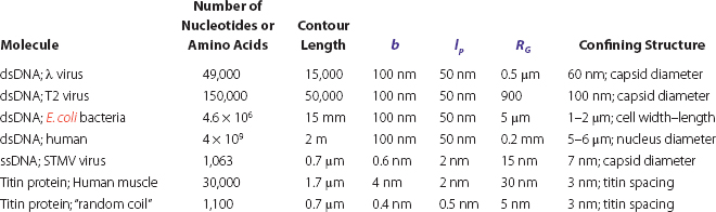
FIGURE 8.1 Molecular dynamics simulations (MDS). Simplified schematic of the general algorithm for performing MDS.

(8.5)

$$r(t+\text{Δ}t)=r(t)+v(t)\text{Δ}t+\frac{F(t)}{m}\frac{{(\text{Δ}t)}^2}{2}+\frac{F(t)}{m}\frac{{(\text{Δ}t)}^3}{3!}+O({\left(\text{Δ}t\right)}^4)$$

Thus, the error is atomic position scales as ~O((Δt)⁴), which is small for the ~femtosecond time increments normally employed, with the equivalent recursive relation for velocities having errors that scale as ~O((Δt)²). The velocity form of the Verlet algorithm most commonly used in MD can be summarized as

(8.6)

$$\begin{array}{lll}r(t+\text{Δ}t)\hfill & =\hfill & r(t)+v(t)\text{Δ}t+(1/2)a(t){(\text{Δ}t)}^2\hfill \\ v(t+\text{Δ}t/2)\hfill & =\hfill & v(t)+(1/2)a(t)\text{Δ}t\hfill \\ a(t+\text{Δ}t)\hfill & =\hfill & -(1/m)\nabla U(r(t=\text{Δ}t))\hfill \\ v(t+\text{Δ}t)\hfill & =\hfill & v(t=\text{Δ}t/2)+(1/2)a(t)\text{Δ}t\hfill \end{array}$$

Related, though less popular, variants of this Verlet numerical integration include the LeapFrog algorithm (equivalent to the Verlet integration but interpolates for velocities at half time step intervals, but has a disadvantage in that velocities are not known at the same time as the atomic positions, hence the name) and Beeman algorithm (generates identical estimates for atomic positions as the Verlet method, but uses a slightly more accurate but computationally more costly method to estimate velocities).

The force is obtained by calculating the grad of the potential energy function U that underlies the summed attractive and repulsive forces. No external applied forces are involved in standard MD simulations; in other words, there is no external energy input into the system, and so the system is in a state of thermodynamic equilibrium.

Most potential energy models used, whether quantum or classical in nature, in practice require some level of approximation during the simulation process and so are often referred to as pseudopotentials or effective potentials. However, important differences exist between MD methods depending on the length and time scales of the simulations, the nature of the force fields used, and whether surrounding solvent water molecules are included or not.

8.2.2  CLASSICAL MD SIMULATIONS

Although the forces on single molecules ultimately have a quantum mechanical (QM) origin—all biology in this sense one could argue is QM in nature—it is very hard to find even approximate solutions to Schrödinger’s equation for anything but a maximum of a few atoms, let alone the ~10²³ found in one mole of biological matter. The range of less straightforward quantum effects in biological systems, such as entanglement, quantum coherence, and quantum superposition, are discussed in Chapter 9. However, in the following section of this chapter, we discuss specific QM methods for MD simulations. But, for many applications, classical MD simulations, also known as simply molecular mechanics (MM), offer a good compromise enabling biomolecule systems containing typically 10⁴–10⁵ atoms to be simulated for ~10–100 ns. The reduction from a quantum to a classical description entails two key assumptions. First, electron movement is significantly faster than that of atomic nuclei such that we assume they can change their relative position instantaneously. This is called the “Born–Oppenheimer approximation,” which can be summarized as the total wave function being the product of the orthogonal wave functions due to nuclei and electrons separately:

(8.7)

$${\text{ψ}}_{total}(nuclei,electrons)=\text{ψ(}nuclei)\text{ψ(}electrons)$$

The second assumption is that atomic nuclei are treated as point particles of much greater mass than the electrons that obey classical Newtonian dynamics. These approximations lead to a unique potential energy function U_total due to the relative positions of electrons to nuclei. Here, the force F on a molecule is found from

(8.8)

$$F=-\nabla U_{total}(\overrightarrow{r})$$

U_total is the total potential energy function in the vicinity of each molecule summed from all relevant repulsive and attractive force sources experienced by each, whose position is denoted by the vector r. A parameter sometimes used to determine thermodynamic properties such as free energy is the potential of mean force (PMF) (not to be confused with the proton motive force; see Chapter 2), which is the potential energy that results in the average force calculated over all possible interactions between atoms in the system.

In practice, most classical MD simulations use relatively simple predefined potentials. To model the effects of chemical bonding between atoms, empirical potentials are used. These consist of the summation of independent potential energy functions associated with bonding forces between atoms, which include the covalent bond strength, bond angles, and bond dihedral potentials (a dihedral, or torsion angle, is the angle between two intersecting planes generated from the relative atomic position vectors). Nonbonding potential energy contributions come typically from van der Waals (vdW) and electrostatic forces. Empirical potentials are limited approximations to QM effects. They contain several free parameters (including equilibrium bond lengths, angles and dihedrals, vdW potential parameters, and atomic charge) that can be optimized either by fitting to QM simulations or from separate experimental biophysical measurements.

The simplest nonbonding empirical potentials consider just pairwise interactions between nearest-neighbor atoms in a biological system. The most commonly applied nonbonding empirical potential in MD simulations is the Lennard-Jones potential U_LJ (see Chapter 2), a version of which is given in Equation 2.10. It is often also written in the form

(8.9)

$$U_{LJ}=4\epsilon \left({\left(\frac{\text{σ}}{r}\right)}^{12}{\left(\frac{\text{σ}}{r}\right)}^6\right)=\epsilon \left({\left(\frac{r_m}{r}\right)}^{12}{\left(\frac{r_m}{r}\right)}^6\right)$$

where

r is the distance between the two interacting atoms

ε is the depth of the potential well

σ is the interatomic distance that results in U_LJ = 0

r_m is the interatomic distance at which the potential energy is a minimum (and thus the force F = 0) given by

(8.10)

$$r_m=2^{1/6}(1.22\sigma )$$

As discussed previously, the r⁻⁶ term models attractive, long-range forces due to vdW interactions (also known as dispersion forces) and has a physical origin in modeling the dipole–dipole interaction due to electron dispersion (a sixth power term). The r⁻¹² term is heuristic; it models the electrostatic repulsive force between two unpaired electrons due to the Pauli exclusion principle, though as such is only used to optimize computational efficiency as the square of the r⁻⁶ term and has no direct physical origin.

For systems containing strong electrostatic forces (e.g., multiple ions), modified versions of Coulomb’s law can be applied to estimate the potential energy U_C–B called the Coulomb–Buckingham potential consisting of the sum of a purely Coulomb potential energy U_C (or electrical potential energy) and the Buckingham potential energy U_B that models the vdW interaction:

(8.11)

$$\begin{array}{lll}{U}_C(\overrightarrow{r})\hfill & =\hfill & \frac{q_1{q}_2}{4{\text{πε}}_0{\text{ε}}_{r}r}\hfill \\ U_B(\overrightarrow{r})\hfill & =\hfill & A_B\exp (-B_{B}r)-\frac{C_B}{r^6}\hfill \\ U_{C-B}(\overrightarrow{r})\hfill & =\hfill & U_B(\overrightarrow{r})+U_C(\overrightarrow{r})=A_B\exp (-B_{B}r)-\frac{C_B}{r^6}+\frac{q_1{q}_2}{4{\text{πε}}_0{\text{ε}}_{r}r}\hfill \end{array}$$

where

q₁ and q₂ are the electrical charges on the two interacting ions

ε_r is the relative dielectric constant of the solvent

ε₀ is the electrical permittivity of free space

A_B, B_B, and C_B are constants, with the –C_B/r⁶ term being the dipole–dipole interaction attraction potential energy term as was the case for the Lennard-Jones potential, but here the Pauli electrical repulsion potential energy is modeled as the exponential term A_Bexp(−B_Br).

However, many biological applications have a small or even negligible electrostatic component since the Debye length, under physiological conditions, is relatively small compared to the length scale of atomic separations. The Debye length, denoted by the parameter κ⁻¹, is a measure of the distance over which electrostatic effects are significant:

(8.12)

$${\text{κ}}^{-1}=\sqrt{\frac{{\text{ε}}_r{\text{ε}}_0{k}_{B}T}{2N_A{q}_e^{2}I}}=\frac{1}{\sqrt{8{\text{πλ}}_B{N}_{A}I}}$$

where

N_A is the Avogadro’s number

q_e is the elementary charge on an electron

I is the ionic strength or ionicity (a measure of the concentration of all ions in the solution)

λ_B is known as the Bjerrum length of the solution (the distance over which the electrical potential energy of two elementary charges is comparable to the thermal energy scale of k_BT)

At room temperature, if κ⁻¹ is measured in nm and I in M, this approximates to

(8.13)

$${\text{κ}}^{-1}\approx \frac{0.304}{\sqrt{I}}$$

In live cells, I is typically ~0.2–0.3 M, so κ⁻¹ is ~1 nm.

In classical MD, the effects of bond strengths, angles, and dihedrals are usually empirically approximated as simple parabolic potential energy functions, meaning that the stiffness of each respective force field can be embodied in a simple single spring constant, so a typical total empirical potential energy in practice might be

(8.14)

$$U_{total}={\displaystyle \sum }_{bonds}{k}_r{(r-r_{eq})}^2+{\displaystyle \sum }_{angles}{k}_{\text{θ}}{(\text{θ}-{\text{θ}}_{eq})}^2+{\displaystyle \sum }_{dihedrals}\frac{V_n}{2}(1+\cos (n\varphi -{\varphi }_{eq}))+{\displaystyle \sum }_{i<j}\left(\frac{A_{ij}}{r_{ij}^{12}}-\frac{B_{ij}}{r_{ij}^6}+\frac{q_i{q}_j}{4{\text{πε}}_{\text{0}}{\text{ε}}_r{r}_{ij}}\right)$$

where

k_r, k_θ are consensus mean stiffness parameters relating to bond strengths and angles, respectively

r, θ, and ϕ are bond lengths, angles, and dihedrals

V_n is the dihedral energy barrier of order n, where n is a positive integer (typically 1 or 2)

r_eq, θ_eq, and ϕ_eq are equilibrium values, determined from either QM simulation or separate biophysical experimentation

For example, x-ray crystallography (Chapter 5) might generate estimates for r_eq, whereas k_r can be estimated from techniques such as Raman spectroscopy (Chapter 4) or IR absorption (Chapter 3).

In a simulation the sum of all unique pairwise interaction potentials for n atoms indicates that the numbers of force, velocity, positions, etc., calculations required scales as ~O(n²). That is to say, if the number of atoms simulated in system II is twice as many as those in system I, then the computation time taken for each Δt simulation step will be greater by a factor of ~4. Some computational improvement can be made by truncation. That is, applying a cutoff for nonbonded force calculations such that only atoms within a certain distance of each other are assumed to interact. Doing this reduces the computational scaling factor to ~O(n), with the caveat of introducing an additional error to the computed force field. However, in several routine simulations, this is an acceptable compromise provided the cutoff does not imply the creation of separate ions.

In principle though, the nonbonding force field is due to a many-body potential energy function, that is, not simply the sum of multiple single pairwise interactions for each atom in the system, as embodied by the simple Lennard-Jones potential, but also including the effects of more than two interacting atoms, not just the single interaction between one given atom and its nearest neighbor. For example, to consider all the interactions involved between the nearest and the next-nearest neighbor for each atom in the system, the computation time required would scale as ~O(n³). More complex computational techniques to account for these higher-order interactions include the particle mesh Ewald (PME or just PM) summation method (see Chapter 2), which can reduce the number of computations required by discretizing the atoms on a grid, resulting in a computation scaling factor of ~O(n^α) where 1 < α < 2, or the PME variant of the Particle-Particle-Particle-Mesh (PPPM or P³M).

PM is a Fourier-based Ewald summation technique, optimized for determining the potentials in many-particle simulations. Particles (atoms in the case of MD) are first interpolated onto a grid/mesh; in other words, each particle is discretized to the nearest grid point. The potential energy is then determined for each grid point, as opposed to the original positions of the particles. Obviously this interpolation introduces errors into the calculation of the force field, depending on how fine a mesh is used, but since the mesh has regular spatial periodicity, it is ideal for Fourier transformation (FT) analysis since the FT of the total potential is then a weighted sum of the FTs of the potentials at each grid point, and so the inverse FT of this weighted sum generates the total potential. Direct calculation of each discrete FT would still yield a ~O(m²) scaling factor for computation for calculating pairwise-dependent potentials where m is the number of grid points on the mesh, but for sensible sampling m scales as ~O(n), and so the overall scaling factor is ~O(n²). However, if the fast Fourier transform (FFT) is used, then the number of calculations required for an n-size dataset is ~n log_e n, so the computation scaling factor reduces to ~O(n log_e n).

KEY POINT 8.1

In P³M, short-range forces are solved in real-space; long-range forces are solved in reciprocal space.

P³M has a similar computation scaling improvement to PM but improves the accuracy of the force field estimates by introducing a cutoff radius threshold on interactions. Normal pairwise calculations using the original point positions are performed to determine the short-range forces (i.e., below the preset cutoff radius). But above the cutoff radius, the PM method is used to calculate long-range forces. To avoid aliasing effects, the cutoff radius must be less than half the mesh width, and a typical value would be ~1 nm. P³M is obviously computationally slower than PM since it scales as ~O(wn log n + (1 – w)n²) where 0 < w < 1 and w is the proportion of pairwise interactions that are deemed long-range. However, if w in practice is close to 1, then the computation scaling factor is not significantly different to that of PM.

Other more complex many-body empirical potential energy models exist, for example, the Tersoff potential energy U_T. This is normally written as the half potential for a directional interaction between atom number i and j in the system. For simple pairwise potential energy models such as the Lennard-Jones potential, the pairwise interactions are assumed to be symmetrical, that is, the half potential in the i → j direction is the same as that in the j → i direction, and so the sum of the two half potentials simply equate to one single pairwise potential energy for that atomic pair. However, the Tersoff potential energy model approximates the half potential as being that due to an appropriate symmetrical half potential due U_S, for example, a U_L–J or U_B–C model as appropriate to the system, but then takes into account the bond order of the system with a term that models the weakening of the interaction between i and j atoms due to the interaction between the i and k atoms with a potential energy U_A, essentially through sharing of electron density between the i and k number atoms:

(8.15)

$$U_T({\overrightarrow{r}}_{ij})=\frac{1}{2}{\displaystyle \sum _{ij}{U}_s({\overrightarrow{r}}_{ij})}+\frac{1}{2}{\displaystyle \sum _{ij}{B}_{ij}{U}_A({\overrightarrow{r}}_{ij})}$$

where the term B_ij is the bond order term, but is not a constant but rather a function of a coordination term G_ij of each bond, that is, B_ij = B(G_ij), such that

(8.16)

$$G_{ij}={\displaystyle \sum }_k{f}_c(r_{ik})g({\text{θ}}_{jik})f(r_{ij}-r_{ik})$$

where

f_c and f are functions dependent on just the relative displacements between the ith and jth and kth atoms

g is a less critical function that depends on the relative bond angle between these three atoms centered on the ith atom

8.2.3  MONTE CARLO METHODS

Monte Carlo methods are in essence very straightforward but enormously valuable for modeling a range of biological processes, not exclusively for molecular simulations, but, for example, they can be successfully applied to simulate a range of ensemble thermodynamic properties. Monte Carlo methods can be used to simulate the effects of complex biological systems using often relatively simple underlying rules but which can enable emergent properties of that system to evolve stochastically that are too difficult to predict deterministically.

If there is one single theoretical biophysics technique that a student would be well advised to come to grips with then it is the Monte Carlo method.

Monte Carlo techniques rely on repeated random sampling to generate a numerical output for the occurrences, or not, of specific events in a given biological system. In the most common applications in biology, Monte Carlo methods are used to enable stochastic simulations. For example, a Monte Carlo algorithm will consider the likelihood that, at some time t, a given biological event will occur or not in the time interval t to t + Δt where Δt is a small but finite discretized incremental time unit (e.g., for combined classical MD methods and Monte Carlo methods, Δt ~ 10⁻¹⁵ s). The probability Δp for that specific biological event to occur is calculated using specific biophysical parameters that relate to that particular biological system, and this is compared against a probability p_rand that is generated from a pseudorandom number generator in the range 0–1. If Δp > p_rand, then one assumes the event has occurred, and the algorithm then changes the properties of the biological system to take account of this event. The new time in the stochastic simulation then becomes t′ = t + Δt, and the polling process in the time interval t′ to t′ + Δt is then repeated, and the process then iterated over the full range of time to be explored.

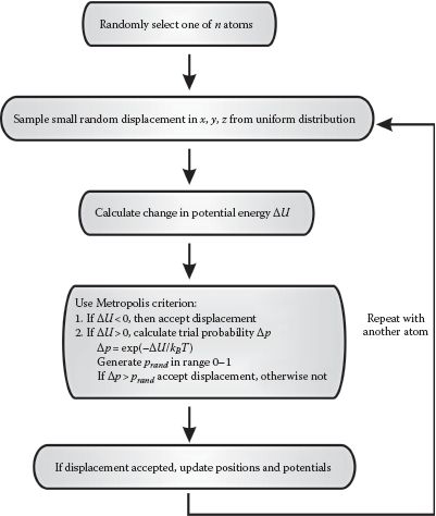
In molecular simulation applications, the trial probability Δp is associated with trial moves of an atom’s position. Classical MD, in the absence of any stochastic fluctuations in the simulation, is intrinsically deterministic. Monte Carlo methods on the other hand are stochastic in nature, and so atomic positions evolve with a random element with time (Figure 8.2). Pseudorandom small displacements are made in the positions of atoms, one by one, and the resultant change ΔU in potential energy is calculated using similar empirical potential energy described in the previous section for classical MD (most commonly the Lennard-Jones potential). Whether the random atomic displacement is accepted or not is usually determined by using the Metropolis criterion. Here, the trial probability Δp is established using the Boltzmann factor exp(−ΔU/k_BT), and if Δp > the pseudorandom probability p_rand, then the atomic displacement is accepted, the potential energy is adjusted and the process iterated for another atom. Since Monte Carlo methods only require potential energy calculations to compute atomic trajectories, as opposed to additional force calculations, there is a saving in computational efficiency.

FIGURE 8.2 Monte Carlo methods in molecular simulations. Simplified schematic of a typical Monte Carlo algorithm for performing stochastic molecular simulations.

This simple process can lead to very complex outputs if, as is generally the case, the biological system is also spatially discretized. That is, probabilistic polling is performed on spatially separated components of the system. This can lead to capturing several emergent properties. Depending on the specific biophysics of the system under study, the incremental time Δt can vary, but has to be small enough to ensure subsaturation levels of Δp that is, Δp < 1 (in practice Δt is often catered so as to encourage typical values of Δp to be in the range ~0.3–0.5). However, very small values of Δt lead to excessive computational times. Similarly, to get the most biological insight ideally requires the greatest spatial discretization of the system. These two factors when combined can result in requirements of significant parallelization of computation and often necessitate supercomputing resources when applied to molecular simulations. However, there are still several biological processes beyond molecular simulations that can be usefully simulated using nothing more than a few lines of code in any standard engineering software language (e.g., C/C++, MATLAB^®, Fortran, Python, LabVIEW) on a standard desktop PC.

A practical issue with the Metropolis criterion is that some microstates during the finite duration of a simulation may be very undersampled or in fact not occupied at all. This is a particular danger in the case of a system that comprises two or more intermediate states of stability for molecular conformations that are separated by relatively large free energy barriers. This implies that the standard Boltzmann factor employed of exp(−ΔU/k_BT) is in practice very small if ΔU equates to these free energy barriers. This can result in a simulation being apparently locked in, for example, one very over sampled state. Given enough time of course, a simulation would explore all microstates as predicted from the ergodic hypothesis (see Chapter 6); however, practical computational limitations may not always permit that.

To overcome this problem, a method called “umbrella sampling” can be employed. Here a weighting factor w is used in front of the standard Boltzmann term:

(8.17)

$$\text{Δ}p(r_i)=w(r_i)\exp \left(\frac{-U(r_i)}{k_{B}T}\right)$$

Thus, for undersampled states, w would be chosen to be relatively high, and for oversampled states, w would be low, such that all microstates were roughly equally explored in the finite simulation time. Mean values of any general thermodynamic parameter A that can be measured from the simulation (e.g., the free energy change between different conformations) can still be estimated as

(8.18)

$$\langle A\rangle =\frac{\langle A/w\rangle }{\langle 1/w\rangle }$$

Similarly, the occupancy probability in each microstate can be estimated using a weighted histogram analysis method, which enables the differences in thermodynamic parameters for each state to be estimated, for example, to explore the variation in free energy differences between the intermediate states.

An extension to Monte Carlo MD simulations is replica exchange MCMC sampling, also known as parallel tempering. In replica exchange, multiple Monte Carlo simulations are performed that are randomly initialized as normal, but at different temperatures. However, using the Metropolis criterion, the molecular configurations at the different temperatures can be dynamically exchanged. This results in efficient sampling of high and low energy conformations and can result in improved estimates to thermodynamical properties by spanning a range of simulation temperatures in a computationally efficient way.

An alternative method to umbrella sampling is the simulated annealing algorithm, which can be applied to Monte Carlo as well as other molecular simulations methods. Here the simulation is equilibrated initially at high temperature but then the temperature is gradually reduced. The slow rate of temperature drop gives a greater time for the simulation to explore molecular conformations with free energy levels lower than local energy minima found by energy minimization, which may not represent a global minimum. In other words, it reduces the likelihood for a simulation becoming locked in a local energy minimum.

8.2.4  AB INITIO MD SIMULATIONS

Small errors in approximations to the exact potential energy function can result in artifactual emergent properties after long simulation times. An obvious solution is therefore to use better approximations, for example, to model the actual QM atomic orbital effects, but the caveat is an increase in associated computation time. Ab initio MD simulations use the summed QM interatomic electronic potentials U_QD experienced by each atom in the system, denoted by a total wave function ψ. Here, U_QD is given by the action of Hamiltonian operator Ĥ on ψ (the kinetic energy component of the Hamiltonian is normally independent of the atomic coordinates) and the force F_QD by the grad of U_QD such that

(8.19)

$$\begin{array}{lll}{U}_{QD}(\overrightarrow{r})\hfill & =\hfill & \widehat{H}\text{ψ}\hfill \\ F_{QD}\hfill & =\hfill & -\nabla (U_{QD}(\overrightarrow{r}))\hfill \end{array}$$

These are, in the simplest cases, again considered as pairwise interactions between the highest energy atomic orbital of each atom. However, since each electronic atomic orbital is identified by a unique value of three quantum numbers, n (the principal quantum number), ℓ (the azimuthal quantum number), and m_ℓ (the magnetic quantum number), the computation time for simulations scales as ~O(n³). However, Hartree–Fock (HF) approximations are normally applied that reduce this scaling to more like ~O(n^2.7). Even so, the computational expense usually restricts most simulations to ~10–100 atom systems with simulation times of ~10–100 ps.

The HF method, also referred to as the self-consistent field method, uses an approximation of the Schrödinger equation that assumes that each subatomic particle, fermions in the case of electronic atomic orbitals, is subjected to the mean field created by all other particles in the system. Here, the n-body fermionic wave function solution of the Schrödinger equation is approximated by the determinant of the n × n spin-orbit matrix called the “Slater determinant.” The HF electronic wave function approximation ψ for an n-particle system thus states

(8.20)

$$\text{ψ}({\overrightarrow{r}}_1,{\overrightarrow{r}}_2,\mathrm{\dots },{\overrightarrow{r}}_n)\approx \frac{1}{\sqrt{n}}\left|\begin{array}{cccc}{\chi }_1({\overrightarrow{r}}_1)& {\chi }_1({\overrightarrow{r}}_1)& \cdots & {\chi }_n({\overrightarrow{r}}_1)\\ {\chi }_1({\overrightarrow{r}}_2)& {\chi }_2({\overrightarrow{r}}_2)& \cdots & {\chi }_n({\overrightarrow{r}}_2)\\ ⋮& ⋮& \ddots & ⋮\\ {\chi }_1({\overrightarrow{r}}_n)& {\chi }_2({\overrightarrow{r}}_n)& \cdots & {\chi }_2({\overrightarrow{r}}_n)\end{array}\right|$$

The term on the right is the determinant of the spin-orbit matrix. The χ elements of the spin-orbit matrix are the wave functions for the various orthogonal (i.e., independent) wave functions for the n individual particles.

In some cases of light atomic nuclei, such as those of hydrogen, QM MD can model the effects of the atomic nuclei as well as the electronic orbitals. A similar HF method can be used to approximate the total wave function; however, since nuclei are composed of bosons as opposed to fermions, the spin-orbit matrix permanent is used instead of the determinant (a matrix permanent is identical to a matrix determinant, but instead the signs in front of the matrix element product permutations being a mixture of positive and negative as is the case for the determinant, they are all positive for the permanent). This approach has been valuable for probing effects such as the quantum tunneling of hydrogen atoms, a good example being the mechanism of operation of an enzyme called “alcohol dehydrogenase,” which is found in the liver and requires the transfer of an atom of hydrogen using quantum tunneling for its biological function.

KEY POINT 8.2

The number of calculations for n atoms in classical MD is ~O(n²) for pairwise potentials, though if a cutoff is employed, this reduces to ~O(n). If next-nearest-neighbor effects (ormore) are considered, ~O(n^α) calculations are required where α ≥ 3. Particle-mesh methods can reduce the number of calculations to ~O(n log n) for classical pairwise interaction models. The number of direct calculations required for pairwise interactions in QM MD is ~O(n³), but approximations to the total wave function can reduce this to ~O(n^2.7).

Ab initio force fields are not derived from predetermined potential energy functions since they do not assume preset bonding arrangements between the atoms. They are thus able to model chemical bond making and breaking explicitly. Different bond coordination and hybridization states for bond making and breaking can be modeled using other potentials such as the Brenner potential and the reactive force field (ReaxFF) potential.

The use of semiempirical potentials, also known as tight-binding potentials, can reduce the computational demands in ab initio simulations. A semiempirical potential combines the fully QM-based interatomic potential energy derived from ab initio modeling using the spin-orbit matrix representation described earlier. However, the matrix elements are found by applying empirical interatomic potentials to estimate the overlap of specific atomic orbitals. The spinorbit matrix is then diagonalized to determine the occupancy level of each atomic orbital, and the empirical formulations are used to determine the energy contributions from these occupied orbitals. Tight-binding models include the embedded-atom method also known as the tight-binding second-moment approximation and Finnis–Sinclair model and also include approaches that can approximate the potential energy in heterogeneous systems including metal components such as the Streitz–Mintmire model.

Also, there are hybrid classical and quantum mechanical methods (hybrid QM/MM). Here, for example, classical MD simulations may be used for most of a structure, but the region of the structure where most fine spatial precision is essential is simulated using QM-derived force fields. These can be applied to relatively large systems containing ~10⁴–10⁵ atoms, but the simulation time is limited by QM and thus restricted to simulation times of ~10–100 ps. Examples of this include the simulation of ligand binding in a small pocket of a larger structure and the investigation of the mechanisms of catalytic activity at a specific active site of an enzyme.

KEY POINT 8.3

Classical (MM) MD methods are fast but suffer inaccuracies due to approximations of the underlying potential energy functions. Also, they cannot simulate chemical reactions involving the making/breaking of covalent bonds. QM MD methods generate very accurate spatial information, but they are computationally enormously expensive. Hybrid QM/MM offers a compromise in having a comparable speed to MM for rendering very accurate spatial detail to a restricted part of a simulated structure.

8.2.5  STEERED MD

Steered molecular dynamics (SMD) simulations, or force probe simulations, use the same core simulation algorithms of either MM or QM simulation methods but in addition apply external mechanical forces to a molecule (most commonly, but not exclusively, a protein) in order to manipulate its structure. A pulling force causes a change in molecular conformation, resulting in a new potential energy at each point on the pulling pathway, which can be calculated at each step of the simulation. For example, this can be used to probe the force dependence on protein folding and unfolding processes, and of the binding of a ligand to receptor, or of the strength of the molecular adhesion interactions between two touching cells. These are examples of thermodynamically nonequilibrium states and are maintained by the input of external mechanical energy into the system by the action of pulling on the molecule.

As discussed previously (see Chapter 2) all living matter is in a state of thermodynamic non-equilibrium, and this presents more challenges in theoretical analysis for molecular simulations. Energy-dissipating processes are essential to biology though they are frequently left out of mathematical/computational models, primarily for three reasons. First, historical approaches inevitably derive from equilibrium formulations, as they are mathematically more tractable. Second, and perhaps most importantly, in many cases, equilibrium approximations seem to account for experimentally derived data very well. Third, the theoretical framework for tackling nonequilibrium processes is far less intuitive than that for equilibrium processes. This is not to say we should not try to model these features, but perhaps should restrict this modeling only to processes that are poorly described by equilibrium models.

Applied force changes can affect the molecular conformation both by changing the relative positions of covalently bonded atoms and by breaking and making bonds. Thus, SMD can often involve elements of both classical and QM MD, in addition to Monte Carlo methods, for example, to poll for the likelihood of a bond breaking event in a given small time interval. The mathematical formulation for these types of bond state calculations relate to continuum approaches of the Kramers theory and are described under reaction–diffusion analysis discussed later in this chapter.

SMD simulations mirror the protocols of single-molecule pulling experiments, such as those described in Chapter 6 using optical and/or magnetic tweezers and AFM. These can be broadly divided into molecular stretches using a constant force (i.e., a force clamp) that, in the experiment, result in stochastic changes to the end-to-end length of the molecule being stretched, and constant velocity experiments, in which the rate of change of probe head displacement relative to the attached molecule with respect to time t is constant (e.g., the AFM tip is being ramped up and down in height from the sample surface using a triangular waveform). If the ramp speed is v and the effective stiffness of the force transducer used (e.g., an AFM tip, optical tweezers) is k, then we can model the external force F_ext due to potential energy U_ext as

(8.21)

$$\begin{array}{lll}{U}_{ext}(t)\hfill & =\hfill & \frac{1}{2}k{(v(t-t_0)-(\overrightarrow{r}(t)-\overrightarrow{r}(t_0).\overrightarrow{u}))}^2\hfill \\ F_{ext}(t)\hfill & =\hfill & -\nabla U_{ext}(t)\hfill \end{array}$$

where

t₀ is some initial time

$\overrightarrow{r}$ is the position of an atom

$\overrightarrow{u}$ is the unitary vector for the pulling direction of the force probe

U_ext can then be summed into the appropriate internal potential energy formulation used to give a revised total potential energy function relevant to each individual atom.

The principle issue with SMD is a mismatch of time scales and force scales between simulation outputs compared to actual experimental data. For example, single-molecule pulling experiments involve generating forces between zero and up to ~10–100 pN over a time scale of typically a second to observe a molecular unfolding event in a protein. However, the equivalent time scale in SMD is more like ~10⁻⁹ s, extending as high as ~10⁻⁶ s in exceptional cases. To stretch a molecule, a reasonable distance compared to its own length scale, for example, ~10 nm, after ~1 ns of simulation implies a probe ramp speed equivalent to ~10 m s⁻¹ (or ~0.1 Å ps⁻¹ in the units often used in SMD). However, in an experiment, ramp rates are limited by viscous drag effects between the probe and the sample, so speeds equivalent to ~10⁻⁶ m s⁻¹ are more typical, seven or more orders of magnitude slower than in the SMD simulations. As discussed in the section on reaction–diffusion analysis later in this chapter, this results in a significantly lower probability of molecular unfolding for the simulations making it nontrivial to interpret the simulated unfolding kinetics. However, they do still provide valuable insight into the key mechanistic events of importance for force dependent molecular processes and enable estimates to be made for the free energy differences between different folded intermediate states of proteins as a function of pulling force, which provides valuable biological insight.

A key feature of SMD is the importance of water solvent molecules. Bond rupture, for example, with hydrogen bonds in particular, is often mediated through the activities of water molecules. The ways in which the presence of water molecules are simulated in general MD are discussed as follows.

8.2.6  SIMULATING THE EFFECTS OF WATER MOLECULES AND SOLVATED IONS

The primary challenge of simulating the effects of water molecules on a biomolecule structure is computational. Molecular simulations that include an explicit solvent take into account the interactions of all individual water molecules with the biomolecule. In other words, the atoms of each individual water molecule are included in the MD simulation at a realistic density, which can similarly be applied to any solvated ions in the solution. This generates the most accuracy from any simulation, but the computational expense can be significant (the equivalent molarity of water is higher than you might imagine; see Worked Case Example 8.1).

The potential energy used is typically Lennard-Jones (which normally is only applied to the oxygen atom of the water molecule interacting with the biomolecule) with the addition of the Coulomb potential. Broadly, there are two explicit solvent models: the fixed charge explicit solvent model and the polarizable explicit solvent model. The latter characterizes the ability of water molecules to become electrically polarized by the nearby presence of the biomolecule and is the most accurate physical description but computationally most costly. An added complication is that there are >40 different water models used by different research groups that can account for the electrostatic properties of water (e.g., see Guillot, 2002), which include different bond angles and lengths between the oxygen and hydrogen atoms, different dielectric permittivity values, enthalpic and electric polarizability properties, and different assumptions about the number of interaction sites between the biomolecule and the water’s oxygen atom through its lone pair electrons. However, the most common methods include single point charge (SPC), TIP3P, and TIP4P models that account for most biophysical properties of water reasonably well.

KEY POINT 8.4

A set of two paired electrons with opposite spins in an outer atomic orbital are considered a lone pair if they are not involved in a chemical bond. In the water molecule, the oxygen atom in principle has two such lone pairs, which act as electronegative sources facilitating the formation of hydrogen bonds and accounting for the fact that bond angle between the two hydrogen atoms and oxygen in a water molecule is greater than 90° (and in fact is closer to 104.5°).

To limit excessive computational demands on using an explicit solvent, periodic boundary conditions (PBCs) are imposed. This means that the simulation occurs within a finite, geometrically well-defined volume, and if the predicted trajectory of a given water molecule takes it beyond the boundary of the volume, it is forced to reemerge somewhere on the other side of the boundary, for example, through the point on the other side of the volume boundary that intersects with a line drawn between the position at which the water molecule moved originally beyond the boundary and the geometrical centroid of the finite volume, for example, if the simulation was inside a 3D cube, then the 2D projection of this might show a square face, with the water molecule traveling to one edge of the square but then reemerging on the opposite edge. PBCs permit the modeling of large systems, though they impose spatial periodicity where there is none in the natural system.

The minimum size of the confining volume of water surrounding the biomolecule needs must be such that it encapsulates the solvation shell (also known as the solvation sphere, also as the hydration layer or hydration shell in the specific case of a water solvent). This is the layer of water molecules that forms around the surface of biomolecules, primarily due to hydrogen bonding between water molecules. However, multiple layers of water molecules can then form through additional hydrogen bond interactions with the primary layer water molecules. The effects of a solvent shell can extend to ~1 nm away from the biomolecule surface, such that the mobility of the water molecules in this zone is distinctly lower than that exhibited in the bulk of the solution, though in some cases this zone can extend beyond 2 nm. The time scale of mixing between this zone and the bulk solution is in the range 10⁻¹⁵ to 10⁻¹² s and so simulations may need to extend to at least these time scales to allow adequate mixing than if performed in a vacuum. The primary hydration shell method used in classical MD with explicit solvent assumes 2–3 layers of water molecules and is reasonably accurate.

An implicit solvent uses a continuum model to account for the presence of water. This is far less costly computationally than using an explicit solvent, but cannot account for any explicit interactions between the solvent and solute (i.e., between the biomolecule and any specific water molecule). In its very simplest form, the biomolecule is assumed only to interact only with itself, but the electrostatic interactions are modified to account for the solvent by assuming the value of the relative dielectric permittivity term ε_r in the Coulomb potential. For example, in a vacuum, ε_r = 1, whereas in water ε_r ≈ 80.

If the straight-line joining atoms for a pairwise interaction are through the structure of the biomolecule itself, with no accessible water present, then the relative dielectric permittivity for the biomolecule itself should be used, for example, for proteins and phospholipid bilayers, ε_r can be in the range ~2–4, and nucleic acids ~8; however, there can be considerable variation deepening on specific composition (e.g., some proteins have ε_r ≈ 20). This very simple implicit solvation model using a pure water solvent is justified in cases where the PMF results in a good approximation to the average behavior of many dynamic water molecules. However, this approximation can be poor in regions close to the biomolecule such as the solvent shell, or in discrete hydration pockets of biomolecules, which almost all molecules in practice have, such as in the interiors of proteins and phospholipid membranes.

The simplest formulation for an implicit solvent that contains dissolved ions is the generalized Born (or simply GB) approximation. GB is semiheuristic (which is a polite way of saying that it only has a physically explicable basis in certain limiting regimes), but which still provides a relatively simple and robust way to estimate long-range electrostatic interactions. The foundation of the GB approximation is the classical Poisson–Boltzmann (PB) model of continuum electrostatics. The PB model uses the Coulomb potential energy with a modified ε_r value but also takes into account the concentration distribution of mobile solvated ions. If U_elec is the electrostatic potential energy, then the Poisson equation for a solution of ions can be written as

(8.22)

$${\nabla }^2{U}_{elec}=-\frac{\text{ρ}}{{\text{ε}}_r{\text{ε}}_0}$$

where ρ is the electric charge density. In the case of an SPC, ρ could be modeled as a Dirac delta function, which results in the standard Coulomb potential formulation. However, for spatially distributed ions, we can model these as having an electrical charge dq in an incremental volume of dV at a position r of

(8.23)

$$dq=\text{ρ}(r)dV(r)$$

Applying the Coulomb potential to the interaction between these incremental charges in the whole volume implies

(8.24)

$$U_{elec}(r_0)=\frac{1}{4{\text{πε}}_r{\text{ε}}_0}{\displaystyle \underset{allspace}{\int }\frac{\text{ρ}dV}{\left|r-r_0\right|}}$$

The Poisson–Boltzmann equation (PBE) then comes from this by modeling the distribution of ion concentration C as

(8.25)

$$\begin{array}{lll}C\hfill & =\hfill & C_0\exp (-z{q}_e{U}_{elec}/k_{B}T)\hfill \\ \therefore \text{ρ}\hfill & =\hfill & FC=F{C}_0\exp (-z{q}_e{U}_{elec}/k_{B}T)\hfill \end{array}$$

where

z is the valence of the ion

q_e is the elementary electron charge

F is the Faraday’s constant

This formulation can be generalized for other types of ions by summing their respective contributions. Substituting Equations 8.23 and 8.24 into Equation 8.25 results in a second-order partial differential equation (PDE), which is the nonlinear Poisson–Boltzmann equation (NLPBE). This can be approximated by the linear Poisson–Boltzmann equation (LPBE) if q_eU_elec/k_BT is very small (known as the Debye–Hückel approximation). Adaptations to this method can account for the effects of counter ions. The LPBE can be solved exactly. There are also standard numerical methods for solving the NLPBE, which are obviously computationally slower than solving the LPBE directly, but the NLPBE is a more accurate electrostatic model than the approximate LPBE.

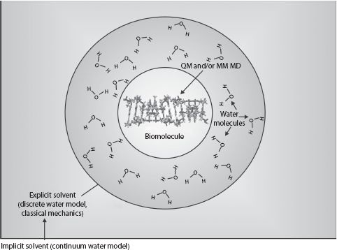
FIGURE 8.3 Multilayered solvent model. Schematic example of a hybrid molecular simulation approach, here shown with a canonical segment of a Z-DNA (see Chapter 2), which might be simulated using either a QM ab initio method or classical (molecular mechanics) dynamics simulations (MD) approach, or a hybrid of the two, while around it is a solvent shell in which the trajectories of water molecules are simulated explicitly using classical MD, and around this shell is an outer zone of implicit solvent in which continuum model is used to account for the effects of water.

A compromise between the exceptional physical accuracy of explicit solvent modeling and the computation speed of implicit solvent modeling is the use a hybrid approach of a multilayered solvent model, which incorporates an additional Onsager reaction field potential (Figure 8.3). Here, the biomolecule is simulated in the normal way of QM or MM MD (or both for hybrid QM/MM), but around each molecule, there is a cavity within which the electrostatic interactions with individual water molecules are treated explicitly. However, outside this cavity, the solution is assumed to be characterized by a single uniform dielectric constant. The biomolecule induces electrical polarization in this outer cavity, which in turn creates a reaction field known as the Onsager reaction field. If a NLPBE is used for the implicit solvent, then this can be a physically accurate model for several important properties. However, even so, no implicit solvent model can account for the effects of hydrophobicity (see Chapter 2), water viscous drag effects on the biomolecule, or hydrogen bonding within the water itself.

8.2.7  LANGEVIN AND BROWNIAN DYNAMICS

The viscous drag forces not accounted for in implicit solvent models can be included by using the methods of Langevin dynamics (LD). The equation of motion for an atom in an energy potential U exhibiting Brownian motion, of mass m in a solvent of viscous drag coefficient γ, involves inertial and viscous forces, but also a random stochastic element, known as the Langevin force, R(t), embodied in the Langevin equation:

(8.26)

$$m\ddot{r}+\gamma \dot{r}=-\nabla U(r)+\sqrt{2\pi k_{B}Tm}R(t)$$

Over a long period of time, the mean of the Langevin force is zero but with a finite variance of $2\text{π}{k}_{B}Tm$. Similarly, the effect on the velocity of an atom is to add a random component that has mean over long period of time of zero but a variance of $2k_{B}T\text{γ}$. Thus, for an MD simulation that involves implicit solvation, LD can be included by a random sampled component from a Gaussian distribution of mean zero and variance $2k_{B}T\text{γ}$.

The value of γ/m = 1/τ is a measure of the collision frequency between the biomolecule atoms and water molecules, where τ is the mean time between collisions. For example, for individual atoms in a protein, τ is in the range 25–50 ps, whereas for water molecules, τ is ~80 ps. The limit of high γ values is an overdamped regime in which viscous forces dominate over inertial forces. Here τ can for some biomolecule systems in water be as low as ~1 ps, which is a diffusion (as opposed to stochastic) dominated limit called Brownian dynamics. The equation of motion in this regime then reduces to the Smoluchowski diffusion equation, which we will discuss later in this chapter in the section on reaction–diffusion analysis.

One effect of applying a stochastic frictional drag term in LD is that this can be used to slow down the motions of fast-moving particles in the simulation and thus act as feedback mechanism to clamp the particle speed range within certain limits. Since the system temperature depends on particle speeds, this method thus equates to a Langevin thermostat (or equivalently a barostat to maintain the pressure of the system). Similarly, other nonstochastic thermostat algorithms can also be used, which all in effect include additional weak frictional coupling constants in the equation of motion, including the Anderson, isokinetic/Gaussian, Nosé–Hoover, and Berendsen thermostats.

8.2.8  COARSE-GRAINED SIMULATION TOOLS

There are a range of coarse-grained (CG) simulation approaches that, instead of probing the exact coordinates of every single atom in the system independently, will pool together groups of atoms as a rigid, or semirigid, structure, for example, as connected atoms of a single amino acid residue in a protein, or coarser still of groups of residues in a single structural motif in a protein. The forces experienced by the components of biological matter in these CG simulations can also be significantly simplified versions that only approximate the underlying QM potential energy. These reductions in model complexity are a compromise to achieving computational tractability in the simulations and ultimately enable larger length and time scales to be simulated at the expense of loss of fine detail in the structural makeup of the simulated biological matter.

This coarse-graining costs less computational time and enables longer simulation times to be achieved, for example, time scales up to ~10⁻⁵ s can be simulated. However, again there is a time scale gap since large molecular conformational changes under experimental conditions can be much slower than this, perhaps lasting hundreds to thousands of microseconds. Further coarse-graining can allow access into these longer time scales, for example, by pooling together atoms into functional structural motifs and modeling the connection between the motifs with, in effect, simple springs, resulting in a simple harmonic potential energy function.

Mesoscale models are at a higher length scale of coarse-graining, which can be applied to larger macromolecular structures. These in effect pool several atoms together to create relatively large soft-matter units characterized by relatively few material parameters, such as mechanical stiffness, Young’s modulus, and the Poisson ratio. Mesoscale simulations can model the behavior of macromolecular systems potentially over a time scale of seconds, but clearly what they lack is the fine detail of information as to what happens at the level of specific single molecules or atoms. However, in the same vein of hybrid QM/MM simulations, hybrid mesoscale/CG approaches can combine elements of mesoscale simulations with smaller length scale CG simulations, and similarly hybrid CG/MM simulations can be performed, with the strategy for all these hybrid methods that the finer length scale simulation tools focus on just highly localized regions of a biomolecule, while the longer length scale simulation tool generates peripheral information about the surrounding structures.

Hybrid QM/MM approaches are particularly popular for investigating molecular docking processes. that is, how well or not a small ligand molecule binds to a region of another larger molecule. This process often utilizes relative simple scoring functions to generate rapid estimates for the goodness of fit for a docked molecule to a putative binding site to facilitate fast computational screening and is of specific interest in in silico drug design, that is, using computational molecular simulations to develop new pharmaceutical chemicals.

8.2.9  SOFTWARE AND HARDWARE FOR MD

Software evolves continuously and rapidly, and so this is not the right forum to explore all modern variants of MD simulation code packages; several excellent online forums exist that give up-to-date details of the most recent advances to these software tools, and the interested reader is directed to these. However, a few key software applications have emerged as having significant utility in the community of MD simulation research, whose core features have remained the same for the past few years, which are useful to discuss here. Three leading software applications have grown directly out of the academic community, including Assisted Model Building with Energy Refinement (AMBER, developed originally at the Scripps Research Institute, United States), Chemistry at HARvard Macromolecular Mechanics (CHARMM developed at the University of Harvard, United States), and GROningen MAchine for Chemical Simulations (GROMACS, developed at the University of Gröningen, the Netherlands).

The term “AMBER” is also used in the MD community in conjunction with “force fields” to describe the specific set of force fields used in the AMBER software application. AMBER software uses the basic force field of Equation 8.14, with presets that have been parameterized for proteins or nucleic acids (i.e., several of the parameters used in the potential energy approximation have been preset by using prior QM simulation or experimental biophysics data for these different biomolecules types). AMBER was developed for classical MD, but now has interfaces that can be used for ab initio modeling and hybrid QM/MM. It includes implicit solvent modeling capability and can be easily implemented on graphics processor units (GPUs, discussed later in this chapter). It does not currently support standard Monte Carlo methods, but has replica exchange capability.

CHARMM has much the same functionality as AMBER. However, the force field used has more complexity, in that it includes additional correction factors:

(8.27)

$$\begin{array}{lll}{U}_{impropers}\hfill & =\hfill & {\displaystyle \sum _{impropers}{k}_W{(\text{ω}-{\text{ω}}_{eq})}^2}\hfill \\ U_{U-B}\hfill & =\hfill & {\displaystyle \sum _{Urey-Bradley}{k}_u{(u-u_{eq})}^2}\hfill \end{array}$$

The addition of the impropers potential, U_impropers, is a dihedral correction factor to compensate for out-of-plane bending (e.g., to ensure that a known planar structural motif remains planar in a simulation) with k_ω being the appropriate impropers stiffness and ω is the out-of-pane angle deviation about the equilibrium angle ω_eq˙ The Urey–Bradley potential, U_U-B, corrects for cross-term angle bending by restraining the motions of bonds by introducing a virtual bond that counters angle bending vibrations, with u a relative atomic distance from the equilibrium position u_eq. The CHARMM force field is physically more accurate than that of AMBER, but at the expense of greater computational cost, and in many applications, the additional benefits of the small correction factors are marginal.

GROMACS again has many similarities to AMBER and CHARMM, but is optimized for simulating biomolecules with several complicated bonded interactions, such as biopolymers in the forms of proteins and nucleic acids, as well as complex lipids. GROMACS can operate with a range of force fields from different simulation software including CHARMM, AMBER, and CG potential energy functions; in addition, its own force field set is called Groningen Molecular Simulation (GROMOS). The basic GROMOS force field is similar to that of CHARMM, but the electrostatic potential energy is modeled as a Coulomb potential with reaction field, U_CRF, which in its simplest form is the sum of the standard ~1/r_ij Coulomb potential U_C with additional contribution from a reaction field, U_RF, which represents the interaction of atom i with an induced field from the surrounding dielectric medium beyond a predetermined cutoff distance R_rf due to the presence of atom j:

(8.28)

$$\begin{array}{lll}{U}_{RF}\hfill & =\hfill & -{\displaystyle \sum _{ij}\frac{q_i{q}_j}{4{\text{πε}}_0{\text{ε}}_1}\frac{C_{rf}{r}_{ij}^2}{R_{rf}^3}}\hfill \\ C_{rf}\hfill & =\hfill & \frac{(2{\text{ε}}_1-2{\text{ε}}_2)(1+\text{κ}{R}_{rf})-{\text{ε}}_2{(\text{κ}{R}_{rf})}^2}{({\text{ε}}_1-2{\text{ε}}_2)(1+\text{κ}{R}_{rf})+{\text{ε}}_2{(\text{κ}{R}_{rf})}^2}\hfill \end{array}$$

where

ε₁ and ε₂ are the relative dielectric permittivity values inside and outside the cutoff radius, respectively

κ is the reciprocal of the Debye screening length of the medium outside the cutoff radius

The software application NAMD (Nanoscale Molecular Dynamics, developed at the University of Illinois at Urbana-Champaign, United States) has also recently emerged as a valuable molecular simulation tool. NAMD benefits from using a popular interactive molecular graphics rendering program called “visual molecular dynamics” (VMD) for simulation initialization and analysis, but its scripting is also compatible with other MD software applications including AMBER and CHARMM, and was designed to be very efficient at scaling simulations to hundreds of processors on high-end parallel computing platforms, incorporating Ewald summation methods. The standard force field used is essentially that of Equation 8.14. Its chief popularity has been for SMD simulations, for which the setup of the steering conditions are made intuitive through VMD.

Other popular packages include those dedicated to more niche simulation applications, some commercial but many homegrown from academic simulation research communities, for example, ab initio simulations (e.g., CASTEP, ONETEP, NWChem, TeraChem, VASP), CG approaches (e.g., LAMMPS, RedMD), and mesoscale modeling (e.g., Culgi). CG tools of oxDNA and oxRNA have utility in mechanical and topological CG simulations of nucleic acids. Others for specific docking processes can be simulated (e.g., ICM, SCIGRESS) and molecular design (e.g., Discovery studio, TINKER) and folding (e.g., Abalone, fold.it, FoldX), with various valuable molecular visualization tools available (e.g., Desmond, VMD).

The physical computation time for MD simulations can take anything from a few minutes for a simple biomolecule containing ~100 atoms up to several weeks for the most complex simulations of systems that include up to ~10,000 atoms. Computational time has improved dramatically over the past decade however due to four key developments:

1.  CPUs have got faster, with improvements to miniaturizing the effective minimum size of a single transistor in a CPU (~40 nm, at the time of writing) enabling significantly more processing power. Today, CPUs typically contain multiple cores. A core is an independent processing unit of a CPU, and even entry-level PCs and laptops use a CPU with two cores (dual-core processors). More advanced computers contain 4–8 core processors, and the current maximum number of cores for any processor is 16. This increase in CPU complexity is broadly consistent with Moore’s law (Moore, 1965). Moore’s law was an interpolation of reduction of transistor length scale with time, made by Gordon E. Moore, the cofounder of Intel, in which the area density of transistors in densely packed integrated circuits would continue to roughly double every ~2 years. The maximum size of a CPU is limited by heat dissipation considerations (but this again has been improved recently by using CPU circulating cooling fluids instead air cooling). The atomic spacing of crystalline silicon is ~0.5 nm that may appear to place an ultimate limit on transistor miniaturization; however, there is increasing evidence that new transistor technology based on smaller length scale quantum tunneling may push the size down even further.

2.  Improvements in simulation software have enabled far greater parallelizability to simulations, especially to route parallel aspects of simulations to different cores of the same CPU, and/or to different CPUs in a network cluster of computers. There is a limit however to how much of a simulation can be efficiently parallelized, since there are inevitably bottlenecks due to one parallelized component of the simulation having to wait for the output from another before it can proceed, though of course multiple different simulations can be run simultaneously at least, for example, for simulations that are stochastic in nature and so are replicated independently several times or trying multiple different starting conditions for deterministic simulations.

3.  Supercomputing resources have improved enormously, with dedicated clusters of ultrafast multiple-core CPUs coupled with locally dedicated ultrahigh bandwidth networks. The use of academic research supercomputers is in general extended to several users where supercomputing time is allocated to enable batch calculations in a block and can be distributed to different computer nodes in the supercomputing cluster.

4.  Recent developments in GPU technology have revolutionized molecular simulations. Although the primary function of a GPU is to assist with the rendering of graphics and visual effects so that the CPU of a computer does not have to, a modern GPU has many features that are attractive to brute number-crunching tasks, including molecular simulations. In essence, CPUs are designed to be flexible in performing several different types of tasks, for example, involving communicating with other systems in a computer, whereas GPUs have more limited scope but can perform basic numerical calculations very quickly. A programmable GPU contains several dedicated multiple-core processors well suited to Monte Carlo methods and MD simulations with a computational power far in excess of a typical CPU. Depending on the design, a CPU core can execute up to 8× 32 bit instructions per clock cycle (i.e., 256 bit per clock cycle), whereas a fast GPU used for 3D video-gaming purposes can execute ~3200× 32 bit instructions per clock, a bandwidth speed difference of a factor of ~400. A very-high-end CPU of, for example, having ~12 cores, has a higher clock rate of up to 2–3 GHz versus 0.7–0.8 GHz for GPUs, but even comparing coupling together four such 12-core CPUs, a single reasonable gaming GPU is faster by at least a factor of 5 and, at the time of writing, cheaper by a factor of at least an order of magnitude. GPUs can now be programmed relatively easily to perform molecular simulations, outperforming more typical multicore CPUs by a speed factor of ~100. GPUs have now also been incorporated into supercomputing clusters. For example, the Blue Waters supercomputer at the University of Urbana-Champaign is, as I write, the fastest supercomputer on any university campus and indeed one of the fastest supercomputers in the world, which can use four coupled GPUs that have performed a VMD calculation of the electrostatic potential for one frame of a MD simulation of the ribosome (an enormously complex biological machine containing over 100,000 atoms with a large length scale of a few tens of nm; see Chapter 2) in just 529 s using just one of these available GPUs, as opposed to ~5.2 h using on a single ultrafast CPU core.

The key advantage with GPUs is that they currently offer better performance per dollar than several of high-end CPU core applied together in a supercomputer, either over a distributed computer network or clustered together in the same machine. A GPU can be installed on an existing computer and may enable larger calculations for less money than building a cluster of computers. However, several supercomputing clusters have GPU nodes now. One caveat is that GPUs do not necessarily offer good performance on any arbitrary computational task, and writing code for a GPU can still present issues with efficient memory use.

One should also be mindful of the size of the computational problem and whether a supercomputer is needed at all. Supercomputers should really be used for very large jobs that no other machine can take on and not be used to make a small job run a bit more quickly. If you are running a job that does not require several CPU cores, you should really use a smaller computer; otherwise, you would just be hogging resources that would be better spent on something else. This idea is the same for all parallel computing, not just for problems in molecular simulation.

Another important issue to bear in mind is that for supercomputing resources you usually have a queue to wait in for your job to start on a cluster. If you care about the absolute time required to get an output from a molecular simulation, the real door-to-door time if you like, it may be worth waiting longer for a calculation to run on a smaller machine in order to save the queue time on a larger one.

KEY POINT 8.5

Driven by the video-gaming industry, GPUs have an improvement in speed of multicore processors that can result in reductions in computational time of ~2 orders of magnitude compared to a multicore CPU.

8.2.10  ISING MODELS

The Ising model was originally developed from quantum statistical mechanics to explain emergent properties of ferromagnetism (see Chapter 5) by using simple rules of local interactions between spin-up and spin-down states. These localized cooperative effects result in emergent behavior at the level of the whole sample. For example, the existence of either ferromagnetic (ordered) or paramagnetic (disordered) bulk emergent features in the sample, and phase transition behavior between the two bulk states, which is temperature dependent up until a critical point (in this example known as the Curie temperature). Many of the key features of cooperativity between smaller length scale subunits leading to a different larger length scale emergent behavior are also present in the Monod–Wyman–Changeux (MWC) model, also known as the symmetry model, which describes the mechanism of cooperative ligand binding in some molecular complexes, for example, the binding of oxygen to the tetramer protein complex hemoglobin (see Chapter 2), as occurs inside red blood cells for oxygenating tissues.

In the MWC model, the phenomenon is framed in terms of allostery; that is, the binding of one subunit affects the ability of it and/or others in the complex to bind a ligand molecule, in which biochemists often characterize by the more heuristic Hill equation for the fraction θ of bound ligand at concentration C that has a dissociation rate constant of K_d (see Chapter 7):

(8.29)

$$\text{θ=}\frac{C^n}{K_d+C^n}$$

where n is the empirical Hill coefficient such that n = 1 indicates no cooperatively, n < 1 is negatively cooperative, n > 1 is positively cooperative.

Hemoglobin has a highly positive cooperativity with n = 2.8 indicating that 2–3 of the 4 subunits in the tetramer interact cooperatively during oxygen binding, which results in a typically sigmoidal shaped all-or-nothing type of response if θ is plotted as a function of oxygen concentration. However, the Ising model puts this interaction on a more generic footing by evoking the concept of an interaction energy that characterizes cooperativity and thus can be generalized into several different systems, biological and otherwise.

In the original Ising model, the magnetic potential energy of a sample in which the ith atom has a magnetic moment (or spin) σ_i is given by the Hamiltonian equation:

(8.30)

$$\stackrel{⌣}{H}=K{\displaystyle \sum _{ij}{\sigma }_i{\sigma }_j-B}{\displaystyle \sum _i{\sigma }_i}$$

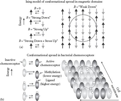
where K is a coupling constant with the first term summation over adjacent atoms with magnetic moments of spin +1 or −1 depending on whether they are up or down and B is an applied external magnetic field. The second term is an external field interaction energy, which increases the probability for spins to line up with the external field to minimize this energy. One simple prediction of this model is that at low B the nearest-neighbor interaction energy will bias nearest neighbors toward aligning with the external field, and this results in clustering of aligned spins, or conformational spreading in the sample of spin states (Figure 8.4a).

FIGURE 8.4 Ising modeling in molecular simulations. (a) Spin-up (black) and spin-down (gray) of magnetic domains at low density in a population are in thermal equilibrium, such that the relative proportion of each state in the population will change as expected by the imposition of a strong external magnetic B-field, which is either parallel (lower energy) or antiparallel (higher energy) to the spin state of the magnetic domain (left panel). However, the Ising model of statistical quantum mechanics predicts an emergent behavior of conformational spreading of the state due to an interaction energy between neighboring domains, which results in spatial clustering of one state in a densely packed population as occurs in a real ferromagnetic sample, even in a weak external magnetic field (dashed circle right panel). (b) A similar effect can be seen for chemoreceptor expressed typically in the polar regions of cell membranes in certain rodlike bacteria such as Escherichia coli. Chemoreceptors are either in an active conformation (black), which results in transmitting the ligand detection signal into the body of the cell or an inactive conformation (gray) that will not transmit this ligand signal into the cell. These two states are in dynamic equilibrium, but the relative proportion of each can be biased by either the binding of the ligand (raises the energy state) or methylation of the chemoreceptor (lowers the energy state) (left panel). The Ising model correctly predicts an emergent behavior of conformational spreading through an interaction energy between neighboring chemoreceptors, resulting in clustering of the state on the surface of the cell membrane (dashed circle, right panel).

This same general argument can be applied to any system that involves a nearest-neighbor interaction between components that exist in two states of different energy, whose state can be biased probabilistically by an external field of some kind. At the long biological length scale, this approach can characterize flocking in birds and swarming in insects and even of social interactions in a population, but at the molecular length scale, there are several good exemplars of this behavior too. For example, bacteria swim up a concentration gradient of nutrients using a mechanism of a biased random walk (see later in this chapter), which involves the use of chemoreceptors that are clustered over the cell membrane. Individual chemoreceptors are two stable conformations, active (which can transmit the detected signal of a bound nutrient ligand molecule to the inside of the cell) and inactive (which cannot transmit the bound nutrient ligand signal to the inside of the cell). Active and inactive states of an isolated chemoreceptor have the same energy. However, binding of a nutrient ligand molecule lowers the energy of the inactive state, while chemical adaptation (here in the form of methylation) lowers the energy of the active state (Figure 8.4b, left panel).

However, in the cell membrane, chemoreceptors are tightly packed, and each in effect interacts with its four nearest neighbors. Because of steric differences between the active and inactive states, its energy is lowered by every neighboring chemoreceptor that is in the same conformational state, but raised by every neighboring receptor in the different state. This interaction can be characterized by an equivalent nearest-neighbor interaction energy (see Shi and Duke, 1998), which results in the same sort of conformational spreading as for ferromagnetism, but now with chemoreceptors on the surface of cell membranes (Figure 8.4b, right panel), and this behavior can be captured in Monte Carlo simulations (Duke and Bray, 1999) and can be extended to molecular systems with more challenging geometries, for example, in a 1D ring of proteins as found in the bacterial flagellar motor (Duke et al., 2001).

This phenomenon of conformational spreading can often be seen in the placement of biophysics academics at conference dinners, if there is a “free” seating arrangement. I won’t go into the details of the specific forces that result in increased or decreased energy states, but you can use your imagination.

KEY BIOLOGICAL APPLICATIONS: MOLECULAR SIMULATION TOOLS

Simulating multiple molecular processes including conformational changes, topology transitions, and ligand docking.

Worked Case Example 8.1 Molecular Simulations

A classical MD simulation was performed on a roughly cylindrical protein of diameter 2.4 nm and length 4.2 nm, of molecular weight 28 kDa, in a vacuum that took 5 full days of computational time on a multicore CPU workstation to simulate 5 ns.

(a)  Estimate with reasoning how long an equivalent simulation would take in minutes if using a particle mesh Ewald summation method. Alternatively, how long might it take if truncation was used?

(b)  At best, how long a simulation in ps could be achieved using an ab initio simulation on the same system for a total computational time of 5 days? A conformational change involving ~20% of the structure was believed to occur over a time scale as high as ~1 ns. Is it possible to observe this event using a hybrid QM/MM simulation with the same total computational time as for part (a)?

(c)  Using classical MD throughout, explicit water was then added with PBCs using a confining cuboid with a square base whose minimum distance to the surface of the protein was 2.0 nm in order to be clear of hydration shell effects. What is the molarity of water under these conditions? Using this information, suggest whether the project undergraduate student setting up the simulation will be able to witness the final result before they leave work for the day, assuming that they want to simulate 5 ns under the same conditions of system temperature and pressure and that there are no internal hydration cavities in the protein, but they decide to use a high-end GPU instead of the multicore CPU.

(Assume that the density and molecular weight of water is 1 g/cm⁻³ and 18 Da, respectively, and that Avogadro’s number is ~6.02 × 10²³.)

Answers

(a)  Mean molecular weight of an amino acid is ~137 Da, which contains a mean of ~19 atoms (see Chapter 2); thus, the number of atoms n in protein is

$n=19\times (28\times 103)/(0.137)=3900\text{atoms}$

PME method scales as ~O(n log_e n), and classical MD scales as ~O(n²) if no truncation used, so a difference of a factor $(n{\log }_{e}n/n^2)=({\log }_{e}n/n)$, so computation time is

$5\text{days}\times {\log }_{\text{e}}(3900/3900)=0.011\text{days}=15\min$

If truncation is used instead, this scales as ~O(n), so a difference of a factor (n/n²) = 1/n, so computation time is

$5\text{days}\times 3900=2\min$

(b)  The best saving in computational time for QM MD using HF approximations scales computation time as ~O(n^2.7), so a difference of a factor (n^2.7/n²) = n^0.7, so total simulation time achievable for a computational time of 5 days is

$5\text{ns}/{39000}^{0.7}=0.015\text{ns}=15\text{ps}$

For hybrid QM/MM, the simulation time is limited by QM. The total number of atoms simulated by the QM MD is 0.2 × 3900 = 780 atoms. The simulation time achievable for the same computational time as for part (a) is thus

$\left(5\text{ns}/{39000}^2/{780}^{2.7}\right)=1.2\text{ns}$

which is >1 ns. Therefore, it is should be possible to observe this conformational change.

(c)  The molarity is defined as the number of moles present in 1 L of the solution. The mass of 1 L of water is 1 kg, but 1 mole of water has a mass of 18 Da, or 18 g; thus, the molarity water is

$(18\times {10}^{-3})=55.6\text{M}\text{.}$

The number of water atoms n_w present is equal to the volume of water in liters multiplied by the molarity of water multiplied by Avogadro’s number. The volume of water V_w present is equal to the volume of the confining cuboid minus the volume of the protein cylinder.

The square based of the confining cuboid must have a minimum edge length w of

$\text{w = 2}\text{.4 nm + (2×2}\text{.0 nm) = 6}\text{.4 nm}$

And the minimum length l of the cuboid is

$l\text{ = 4}\text{.2 nm + (2×2}\text{.0 nm) = 8}\text{.2 nm}$

Thus, volume V_c of the cuboid is

$V_{\text{c}}\text{ = (6}{\text{.4×10}}^{-\text{9}}{\text{)}}^{\text{2}}\text{ × (8}{\text{.2×10}}^{-\text{9}}\text{) = 3}{\text{.2×10}}^{-\text{25}}{\text{ m}}^{\text{3}}\text{ = 3}{\text{.2×10}}^{-\text{22}}\text{ L}\text{.}$

Similarly, the volume of the protein cylinder V_p is given by

$V_p\text{= (π×(0}\text{.5×2}{\text{.4 nm)}}^{\text{2}}\text{)×4}\text{.2 nm = 1}{\text{.9×10}}^{-\text{22}}\text{ L}$

Thus,

$V_{\text{c}}\text{= (3}\text{.2}-\text{1}{\text{.9)×10}}^{-\text{22}}\text{=1}{\text{.3×10}}^{-\text{22}}\text{ L}$

Thus,

$n_w\text{= 55}\text{.6×(6}{\text{.02×10}}^{\text{23}}\text{)×1}{\text{.3×10}}^{-\text{22}}\text{=4350 atoms}$

All of these atoms plus the 3900 atoms of the protein must be included explicitly in the simulation. A high-end GPU is faster than a typical multicore processor by a factor of ~100. Thus, the total computing time required is

$\text{(5 days/100)}\times {\text{(3900+4350)}}^{\text{2}}{\text{/(3900)}}^{\text{2}}\text{ = 0}\text{.52 days = 12}\text{.5 h}$

Would the project student be able to witness the results of the simulation before they go home from work? Yes, of course. Project students don’t need sleep….

8.3  MECHANICS OF BIOPOLYMERS

Many important biomolecules are polymers, for example, proteins, nucleic acids, lipids, and many sugars. Continuum approaches of polymers physics can be applied to many of these molecules to infer details concerning their mechanical properties. These include simple concepts such as the freely jointed chain (FJC) and freely rotating chain (FRC) with approximations such as the Gaussian chain (GC) and wormlike chain (WLC) approaches and how these entropic spring models predict responses of polymer extension to imposed force. Nonentropic sources of biopolymer elasticity to model less idealized biopolymers are also important. These methods enable theoretical estimates of a range of valuable mechanical parameters to be made and provide biological insight into the role of many biopolymers.

8.3.1  DISCRETE MODELS FOR FREELY JOINTED CHAINS AND FREELY ROTATING CHAINS

The FJC model, also called the “random-flight model” or “ideal chain,” assumes n infinitely stiff discrete chain segments each of length b (known as the Kuhn length) that are freely jointed to, and transparent to, each other (i.e., parts of the chain can cross through other parts without impediment) such that the directional vector r_i of the ith segment is uncorrelated with all other segments (Figure 8.5a). The end-to-end distance of the chain R is therefore equivalent to a 3D random walk. We can trivially deduce the first moment of the equivalent vector R (the time average over a long time) as

(8.31)

$$\langle R\rangle =\langle {\displaystyle \sum }_{i-1}^n{r}_i\rangle =0$$

FIGURE 8.5 Modeling biopolymer mechanics. (a) Schematic of freely jointed and wormlike chains (WLCs) indicating Kuhn (b) and persistence lengths (l_p), respectively. (b) Typical fits of WLC and freely jointed chain models to real experimental data obtained using optical tweezers stretching of a single molecule of the muscle protein titin (dots), which (c) can undergo hysteresis due to the unfolding of domains in each structure. (Data courtesy of Mark Leake, University of York, York, U.K.)

Since there is no directional bias to r_i. The second moment of R (the time average of the dot-product R² over long time) is similarly given by

(8.32)

$$\langle R^2\rangle =\langle R\cdot R\rangle =\langle R^2\rangle =\langle {\left({\displaystyle \sum }_{i=1}^n{r}_i\right)}^2\rangle ={\displaystyle \sum }_{i=1}^n\langle r_i{}^2\rangle +2{\displaystyle \sum }_{i=1}^n{\displaystyle \sum }_{j=i}^{n-i}\langle r_i\cdot r_{i\_j}\rangle$$

The last term equates to zero since r_i · r_j is given by r_ir_j cos θ_ij where θ_ij is the angle between the segment vectors, and $\langle \cos {\text{θ}}_{ij}\rangle =0$ over long time for uncorrelated segments. Thus, the mean square end-to-end distance is given simply by

(8.33)

$$\langle R^2\rangle =n\langle {\mathbf{\text{r}}}_i{}^2\rangle =n{b}^2$$

So the root mean square (rms) end-to-end distance scales simply with $\sqrt{n}$:

(8.34)

$$\sqrt{\langle R_{FJC}^2\rangle }=\sqrt{nb}$$

Another valuable straightforward result also emerges for the radius of gyration of the FJC, which is the mean square distance between all of the segments in the chain. This is identical to the mean distance of the chain from its center of mass, denoted by vector R_G:

(8.35)

$$\begin{array}{lll}{R}_G\hfill & =\hfill & \frac{1}{n}{\displaystyle \sum _{j=1}^n{R}_j}\hfill \\ \therefore R_G^2\hfill & =\hfill & \frac{1}{n}{\displaystyle \sum _{i=1}^n\langle {(R_i-R_G)}^2\rangle =\frac{1}{n}{\displaystyle \sum _{i=1}^n\langle {\left(R_i-\frac{1}{n}{\displaystyle \sum _{j=1}^n{R}_j}\right)}^2\rangle }}\hfill \\ \hfill & =\hfill & \frac{1}{n}{\displaystyle \sum _{i=1}^n\langle {\left(R_i^2-\frac{2R_i}{n}\cdot {\displaystyle \sum _{j=1}^n{R}_j+\frac{1}{n^2}{\displaystyle \sum _{j=1}^n{\displaystyle \sum _{k=1}^n{R}_j\cdot R_k}}}\right)}^2\rangle }\hfill \\ \hfill & =\hfill & \langle \frac{1}{n}{\displaystyle \sum _{i=1}^n{R}_i^2-\frac{1}{n^2}{\displaystyle \sum _{j=1}^n{\displaystyle \sum _{k=1}^n{R}_j\cdot R_k}}}\rangle \hfill \\ \hfill & =\hfill & \frac{1}{2n^2}{\displaystyle \sum _{j=1}^n{\displaystyle \sum _{k=1}^n\langle {(R_j-R_k)}^2\rangle }}\hfill \end{array}$$

Using the result of Equation 8.34, we can then say

(8.36)

$$R_G^2=\frac{1}{2n^2}{\displaystyle \sum _{j=1}^n{\displaystyle \sum _{k=1}^n\left|j-k\right|b^2=\frac{b^{2}n(n-2)}{6(n-1)}}}$$

A valuable general approximation comes from using high values of n in this discrete equation or by approximating the discrete summations as continuum integrals, which come to the same result of

(8.37)

$$\begin{array}{lll}{R}_G^2\hfill & \approx \hfill & \frac{1}{2n^2}\underset{0}{\overset{n}{{\displaystyle \int }}}dj\underset{0}{\overset{n}{{\displaystyle \int }}}dk|j-k|b^2=\frac{b^2}{n^2}\underset{0}{\overset{n}{{\displaystyle \int }}}dj\underset{0}{\overset{j}{{\displaystyle \int }}}dk(j-k)=\frac{n{b}^2}{6}=\frac{\langle R_{FJC}^2\rangle }{6}\hfill \\ \therefore \sqrt{R_G^2}\hfill & \approx \hfill & \frac{\sqrt{\langle R_{FJC}^2\rangle }}{\sqrt{6}}\approx 0.41\sqrt{\langle R_{FJC}^2\rangle }\hfill \end{array}$$

Another useful result that emerges from similar analysis is the case of the radius of gyration of a branched polymer, where the branches are of equal length and joined at a central node such that if there are f such branches, the system is an f arm star polymer. This result is valuable for modeling biopolymers that form oligomers by binding together at one specific end, which can be reduced to

(8.38)

$$R_{G,f-arm}=\frac{b^2}{2n^2}\underset{0}{\overset{n/f}{{\displaystyle \int }}}dj\underset{0}{\overset{n/f}{{\displaystyle \int }}}dk(j+k)f(f+1)+\frac{f{b}^2}{n^2}\underset{0}{\overset{n/f}{{\displaystyle \int }}}dj\underset{0}{\overset{j}{{\displaystyle \int }}}dk(j-k)$$

The first and second terms represent inter- and intra-arm contributions respectively, which can be evaluated as

(8.39)

$$R_{G,f-arm}=\frac{n{b}^2}{6}\frac{(3f-2)}{f^2}=\text{α(}f)\langle R_G^2\rangle$$

Thus, at small f (= 1 or 2), α is 1, for much larger f, α is ~3/f and R_G,f-arm decreases roughly as ~3R_G/f.

The FRC has similar identical stiff segment assumptions as for the FJC; however, here the angle θ between position vectors of neighboring segments is fixed but the torsional angle ψ (i.e., the angle of twist of one segment around the axis of a neighboring segment) is free to rotate. A similar though slightly more involved analysis to that of the FJC, which considers the recursive relation between adjacent segments, leads to

(8.40)

$$\langle R^2\rangle =n{b}^2\left(1+\frac{2\cos \text{θ}}{1-\cos \text{θ}}\left(1-\frac{1-{\left(\cos \text{θ}\right)}^n}{n\left(1-\cos \text{θ}\right)}\right)\right)$$

For high values of n, this equation can be reduced to the approximation

(8.41)

$$\begin{array}{lll}\langle R^2\rangle \hfill & \approx \hfill & n{b}^2\left(\frac{1+\cos \text{θ}}{1-\cos \text{θ}}\right)\hfill \\ \therefore \sqrt{\langle R_{FRC}^2\rangle }\hfill & \approx \hfill & b\sqrt{n\left(\frac{1+\cos \text{θ}}{1-\cos \text{θ}}\right)}\equiv \sqrt{\langle R_{FJC}^2\rangle }g(\text{θ})\hfill \end{array}$$

This additional angular constraint often results in better agreement to experimental data, for example, using light scattering measurements from many proteins (see Chapter 3), due to real steric constraints due to the side groups of amino acid residues whose effective value of g is in the range ~2–3.

8.3.2  CONTINUUM MODEL FOR THE GAUSSIAN CHAIN

The GC is a continuum approximation of the FJC (which can also be adapted for the FRC) for large n (>100), applying the central limit theorem to the case of a 1D random walk in space. Considering n unitary steps taken on this random walk that are parallel to the x-axis, a general result for the probability p(n, x) for being a distance x away from the origin, which emerges from Stirling’s approximation to the log of the binomial probability density per unit length at large n, is

(8.42)

$$\begin{array}{lll}p(n,x)\hfill & =\hfill & \frac{1}{\sqrt{2\text{π}n}}\exp \left(\frac{-x^2}{2n^2}\right)\hfill \\ \therefore \langle x^2\rangle \hfill & =\hfill & {\displaystyle \underset{-\infty }{\overset{+\infty }{\int }}{x}^{2}pdx=n}\hfill \end{array}$$

This integral is evaluated using as a standard Gaussian integral. Thus, we can say

(8.43)

$$p(n,x)=\frac{1}{\sqrt{2\text{π}\langle x^2\rangle }}\exp \left(\frac{-x^2}{2\langle x^2\rangle }\right)$$

However, a FJC the random walk is in 3D, and so the probability density per unit volume p(n, R) is the product of the three independent probability distributions in x, y, and z, and each step is of length b, leading to

(8.44)

$$p(n,R)={\left(\frac{3}{2\text{π}\langle R^2\rangle }\right)}^{3/2}\exp \left(\frac{-3R^2}{2\langle R^2\rangle }\right)={\left(\frac{3}{2\text{π}n{b}^2}\right)}^{3/2}\exp \left(\frac{-3R^2}{2n{b}^2}\right)$$

For example, the probability of finding the end of the polymer in a spherical shell between R and R + dR is then p(n, R) · 4πR²dR. This result can be used to predict the effective hydrodynamic (or Stokes) radius R_H. Here, the effective rate of diffusion of all arbitrary sections between the ith and jth segments is additive, and since the diffusion coefficient is proportional to the reciprocal of the effective radius of a diffusing particle from the Stokes–Einstein equation (Equation 2.12), this implies

(8.45)

$$\begin{array}{lll}\frac{1}{R_H}\hfill & =\hfill & \langle \frac{1}{\left|r_i-r_j\right|}\rangle ={\displaystyle \underset{0}{\overset{\infty }{\int }}{\left(2\text{π}\langle \left|i-j\right|\rangle b^2/3\right)}^{-3/2}\exp \left(\frac{-3r^2}{2\langle \left|i-j\right|\rangle b^2}\right)}\cdot 4\text{π}{r}^2\frac{1}{r}dr\hfill \\ \hfill & =\hfill & {\left(\frac{6}{\text{π}}\right)}^{1/2}{b}^{-1}{\langle \left|i-j\right|\rangle }^{-1/2}={\left(\frac{6}{\text{π}}\right)}^{1/2}{b}^{-1}{n}^{-2}{\displaystyle \underset{0}{\overset{n}{\int }}di}{\displaystyle \underset{0}{\overset{n}{\int }}dj{\left|i-j\right|}^{-1/2}=}{\left(\frac{6}{\text{π}}\right)}^{1/2}{b}^{-1}\left(\frac{8}{\text{3}}\right)n^{-1/2}\hfill \\ \therefore R_H\hfill & =\hfill & \frac{1}{8}\sqrt{\left(\frac{3\text{π}}{2}\right)}\sqrt{nb}=\frac{1}{8}\sqrt{\left(\frac{3\text{π}}{2}\right)}\sqrt{\langle R_{FJC}^2\rangle }\approx 0.27\sqrt{\langle R_{FJC}^2\rangle }\hfill \end{array}$$

Thus

$\sqrt{\langle R_{FRC}^2\rangle }>\sqrt{\langle R_{FJC}^2\rangle }>R_G>R_{H\cdot }$

8.3.3  WORMLIKE CHAINS

Biopolymers with relatively long segment lengths are accurately modeled as a wormlike chain, also known as the continuous version of the Kratky–Porod model. This model can be derived from the FRC by assuming small θ, with the result that

(8.46)

$$\langle R_{WLC}^2\rangle =2l_p{R}_{\max }-2l_p^2\left(1-\exp \left(\frac{-R_{\max }}{l_p}\right)\right)$$

where

l_p is known as the persistence length

R_max is the maximum end-to-end length, which is equivalent to the contour length from the FJC of nb

In the limit of a very long biopolymer (i.e., R_max ≫ l_p),

(8.47)

$$\begin{array}{l}\langle R_{WLC}^2\rangle \approx 2l_p{R}_{\max }-2l_p(nb)\equiv \langle R_{FJC}^2\rangle =n{b}^2\hfill \\ \therefore l_p\approx \frac{b}{2}\hfill \end{array}$$

This is the ideal chain limit for a relatively compliant biopolymer. Similarly, in the limit of a short biopolymer (i.e., R_max ≪ l_p),

(8.48)

$$\langle R_{WLC}^2\rangle \approx R_{\max }^2$$

This is known as the rodlike limit corresponding to a very stiff biopolymer.

8.3.4  FORCE DEPENDENCE OF POLYMER EXTENSION

The theory of flexible polymers described previously for biopolymer mechanics results in several different polymer conformations having the same free energy state (i.e., several different microstates). At high end-to-end extension close to a biopolymer’s natural contour length, there are fewer conformations that the molecule can adopt compared to lower values. Therefore, there is an entropic deficit between high and low extensions, which is manifest as an entropic force in the direction of smaller end-to-end extension.

KEY POINT 8.6

There are fewer accessible microstates for high values of end-to-end extension compared to low values for a stretched biopolymer resulting in an entropic restoring force toward smaller extension values. The force scale required to straighten an FJC runs from zero to ~k_BT/b.

The force response F of a biopolymer to a change in end-to-end extension r can be characterized in the various models of elasticity described earlier. If the internal energy of the biopolymer stays the same for all configurations (in other words that each segment in the equivalent chain is infinitely rigid), then entropy is the only contribution to the Helmholtz free energy A:

(8.49)

$$A(R)=-TS(R)=k_{B}T\text{ln }p\left(n,R\right)$$

where p is the radial probability density function discussed in the previous section. The restoring force experienced by a stretched molecule of end-to-end length R is then given by

(8.50)

$$F=\frac{\partial A}{\partial R}$$

with a molecular stiffness k given by

(8.51)

$$k=\frac{\partial F}{\partial R}$$

Using the result for p for the GC model of Equation 8.44 indicates

(8.52)

$$A=\frac{3k_{B}T{R}^2}{2R_{\max }b}$$

Therefore, the GC restoring force is given by

(8.53)

$$F_{GC}=\frac{3k_{B}TR}{R_{\max }b}$$

Thus, the GC molecular stiffness is given by

(8.54)

$$k_{GC}=\frac{3k_{B}T}{n{b}^2}=\frac{3k_{B}T}{\langle R_{FJC}^2\rangle }$$

This implies that a GC exhibits a constant stiffness with extension, that is, it obeys Hooke’s law, with the stiffness proportional to the thermal energy scale of k_BT and to the reciprocal of b². This is a key weakness with the GC model; a finite force response even after the biopolymer is stretched beyond its own contour length is clearly unphysical. The FJC and WLC models are better for characterizing a biopolymer’s force response with extension. Evaluating p for the FJC and WLC models is more complicated, but these ultimately indicate that, for the FJC model,

(8.55)

$$R\approx R_{\max }\left(\coth \left(\frac{F_{FJC}b}{k_{B}T}\right)-\frac{k_{B}T}{F_{FJC}b}\right)s$$

Similarly, for the WLC model,

(8.56)

$$F_{WLC}\approx \left(\frac{k_{B}T}{l_p}\right)\left(\frac{1}{4{(1-R/R_{\max })}^2}-\frac{1}{4}+\frac{R}{R_{\max }}\right)$$

The latter formulation is most popularly used to model force-extension data generated from experimental single-molecule force spectroscopy techniques (see Chapter 6), and this approximation deviates from the exact solution by <10% for forces <100 pN. Both models predict a linear Hookean regime at low forces. Examples of both FJC and WLC fits to the same experimental data obtained from optical tweezers stretching of a single molecule of titin are shown in Figure 8.5b.

By integrating the restoring force with respect to end-to-end extension, it is trivial to estimate the work done, ΔW in stretching a biopolymer from zero up to end-to-end extension R. For example, using the FJC model, at low forces (F < k_BT/b and R < R_max/3),

(8.57)

$$\text{Δ}W=\frac{3k_{B}T}{2n{b}^2}{R}^2=\frac{3k_{B}T}{2}{\left(\frac{R}{\langle R\rangle }\right)}^2$$

In other words, the free energy cost per spatial dimension degree of freedom reaches k_BT/2 when the end-to-end extension reaches its mean value. This is comparable to the equivalent energy E to stretch an elastic cylindrical rod of radius r modeled by Hooke’s law:

(8.58)

$$\begin{array}{lll}\frac{\text{Δ}R}{R}\hfill & =\hfill & \frac{\text{σ}}{Y}=\frac{F}{F_0}\hfill \\ \therefore E\hfill & =\hfill & {\displaystyle \underset{0}{\overset{\text{Δ}R}{\int }}fd(\text{Δ}R)=\frac{F_0{(\text{Δ}R)}^2}{2}}\hfill \end{array}$$

where

Y is the Young’s modulus

σ is the stress F/πr²

F₀ is πr²Y

However, at high forces and extensions, the work done becomes

(8.59)

$$\text{Δ}W\approx C-\frac{k_{B}T}{b}\ln \left(1-\frac{R}{R_{\max }}\right)$$

where C is a constant. As the biopolymer chain extension approaches its contour length R_max, the free energy cost in theory diverges.

8.3.5  REAL BIOPOLYMERS

As discussed earlier, the GC chain model does not account well for the force response of real molecules to changes in molecular extension, which are better modeled by FJC, FRC, and WLC models. In practice, however, real biopolymers may have heterogeneity in b and l_p values, that is, there can be multiple different structural components within a molecule. We can model these effects in the force dependence as having N-such separate chains attached in parallel, both with FJC and WLC models. Thus, for N-FLC,

(8.60)

$$R={\displaystyle \sum _{i=1}^N{R}_i}={\displaystyle \sum _{i=1}^N{R}_{\max ,i}}\left(\coth \left(\frac{F{b}_i}{k_{B}T}\right)-\frac{k_{B}T}{F{b}_i}\right)$$

Similarly, for N-WLC,

(8.61)

$$\begin{array}{lll}F\hfill & =\hfill & \left(\frac{k_{B}T}{l_{p,i}}\right)\left(\frac{1}{4(1-R_i/R_{\max ,i})}-\frac{1}{4}+\frac{R_i}{R_{\max ,i}}\right)\hfill \\ R\hfill & =\hfill & {\displaystyle \sum _{i=1}^N{R}_i}\hfill \end{array}$$

However, in practice, real biopolymers do not consist of segments that are freely jointed as in the FJC. There is real steric hindrance to certain conformations that are not accounted for in the FJC model, though to some extent these can be modeled by the additional angular constraints on the FRC model, which are also embodied in the WLC model. However, all of these models have the key assumption that different sections of the molecule can transparently pass through each other, which is obviously unphysical. More complex excluded volume WLC approaches can disallow such molecular transparency.

Also, the assumption that chain segments, or equivalent sections of the chain of l_p length scale, are infinitely stiff is unrealistic. In general, there may also be important enthalpic spring contributions to molecular elasticity. For example, the behavior of the chain segments can be more similar to Hookean springs, consistent with an increasing separation of constituent atoms with greater end-to-end distance resulting in an opposing force due to either bonding interactions (i.e., increasing the interatomic separation beyond the equilibrium value, similarly for bond angle and dihedral components) and for nonbonding interactions, for example, the Lennard-Jones potential predicts a smaller repulsive force and greater vdW attractive force at increasing interatomic separations away from the equilibrium separation, and similar arguments apply to electrostatic interactions. These enthalpic effects can be added to the purely entropic components in modified elastically jointed chain models. For example, for a modified FJC model in which a chain is composed of freely jointed bonds that are connected by joints with some finite total enthalpic stiffness K,

(8.62)

$$R=R_{\max }\left(\coth \left(\frac{Fb}{k_{B}T}\right)-\frac{k_{B}T}{Fb}\right)\left(1+\frac{F}{K}\right)$$

or similarly, for an enthalpic-modified WLC model,

(8.63)

$$F=\left(\frac{k_{B}T}{l_p}\right)\left(\frac{1}{4{(1-R/R_{\max }+F/K)}^2}-\frac{1}{4}+\frac{R}{R_{\max }}-\frac{F}{K}\right)$$

Deviations exist between experimentally determined values of b and l_p parameters and those predicted theoretically on the basis of what appear to be physically sensible length scales for known structural information. For example, the length of a single amino acid in a protein, or the separation of a single nucleotide base pair in a nucleic acid, might on first inspection seem like sensible candidates for an equivalent segment of a chain. Also, there are inconsistencies between experimentally estimated values for R_G of some biopolymers compared against the size of cellular structures that contain these molecules (Table 8.1).

TABLE 8.1  Biopolymer Model Parameters of Real Molecules

Notes:  Selection of polymer elasticity parameters from different types of DNA (ss/ds = single-strand/double-stranded) and muscle protein titin used in various biophysical elasticity experiments. R_G has been calculated from the measured b values. The general trend is that the estimated R_G is much larger than the length scale of their respective cellular “containers”