Biophysics Tools and Techniques

Valuable Experimental Methods That Complement Mainstream Research Biophysics Techniques

General Idea: There are several important accessory experimental methods that complement techniques of biophysics, many of which are invaluable to the efficient functioning of biophysical methods. They include controllable chemical techniques for gluing biological matter to substrates, the use of “model” organisms, genetic engineering tools, crystal preparation for structural biology studies, and a range of bulk sample methods, including some of relevance to biomedicine.

The key importance for a student of physics in regard to learning aspects of biophysical tools and technique is to understand the physics involved. However, the devil is often in the detail, and the details of many biophysical methods include the application of techniques that are not directly biophysical as such, but which are still invaluable, and sometimes essential, to the optimal functioning of the biophysical tool. In this chapter we discuss the key details of these important, complementary approaches. We also include discussion of the applications of biophysics in biomedical techniques. There are several textbooks dedicated to expert-level medical physics technologies; however, what we do here is highlight the important biophysical features of these to give the reader a basic all-round knowledge of how biophysics tools are applied to clinically relevant questions.

Bioconjugation is an important emerging field of research in its own right. New methods for chemical derivatization of all the major classes of biomolecules have been developed, many with a significant level of specificity. As we have seen from the earlier chapters in this book that outline experimental biophysics tools, bioconjugation has several applications to biophysical techniques, especially those requiring molecular level precision, for example, labeling biomolecules with a specific fluorophore tag or EM marker, conjugating a molecule to a bead for optical and magnetic tweezers experiments, chemically modifying surfaces in order to purify a mixture of molecules.

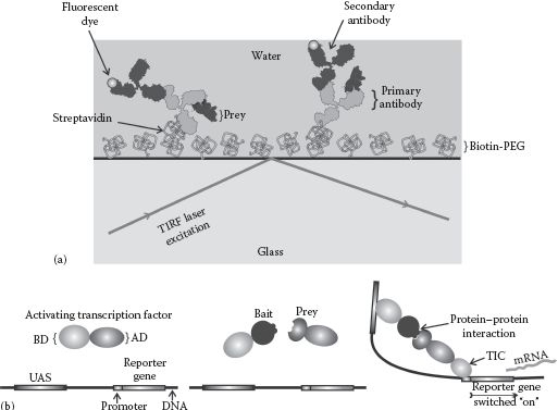
Biotin is a natural molecule of the B-group of vitamins, relatively small with a molecular weight roughly twice that of a typical amino acid residue (see Chapter 2). It binds with high affinity to two structurally similar proteins called “avidin” (found in egg white of animals) and “streptavidin” (found in bacteria of the genus Streptomyces; these bacteria have proved highly beneficial to humans since they produce >100,000 different types of natural antibiotics, severally used in clinical practice). Chemical binding affinity in general can be characterized in terms of a dissociation constant, K_d. This is defined as the product of all the two concentrations of the separate components in solution that bind together divided by the concentration of the bound complex itself and thus has the same units as concentration (e.g., molarity, or M). The biotin–avidin or biotin–streptavidin interaction has a K_d of 10⁻¹⁴ to 10⁻¹⁵ M. Thus, the concentration of “free” biotin in solution in the presence of avidin or streptavidin is exceptionally low, equivalent to just a single molecule inside a volume of a very large cell of ~100 μm diameter.

Thirty percent of the amino acid sequence of avidin is identical to streptavidin; however, their secondary, tertiary, and quaternary structures are almost the same: each molecule containing four biotin binding sites. Avidin has a higher intrinsic chemical affinity to biotin than streptavidin, though this situation is often reversed when avidin/streptavidin are bound to a conjugate. However, a modified version of avidin called “NeutrAvidin” has a variety of chemical groups removed from the structure including outer carbohydrate groups, which reduces nonspecific noncovalent binding to a range of biomolecules compared to both avidin and streptavidin. As a result, this is often the biotin binder of choice in many applications.

These strong interactions are very commonly used by biochemists in conjugation chemistry. Biotin and streptavidin/avidin pairs can be chemically bound to a biomolecule using accessible reactive groups on the biomolecules, for example, the use of carboxyl, amine, or sulfhydryl groups in protein labeling (see in the following text). Separately, streptavidin/avidin can also be chemically labeled with, for example, a fluorescent tag and used to probe for the “biotinylated” sites on the protein following incubation with the sample.

Carboxyl (—COOH), amine (—NH₂), and sulfhydryl (—SH) groups are present in many biomolecules and can all form covalent bonds to bridge to another chemical group through loss of a hydrogen atom. For example, conjugation to a protein can be achieved via certain amino acids that contain reactive amine groups—these are called “primary” (free) amine groups that are present in the side “substituent” group of amino acids and do not partake in peptide bond formation. For example, the amine acid lysine contains one such primary amine (see Chapter 2), which under normal cellular pH levels is bound to a proton to form the ammonium ion of —NH₃+. Primary amines can undergo several types of chemical conjugation reactions, for example, acylation, isocyanate formation, and reduction.

Similarly, some amino acids (e.g., aspartic acid and glutamic acid) contain one or more reactive carboxyl groups that do not participate in peptide bond formation. These can be coupled to primary amine groups using a cross-linker chemical such as carbodiimide (EDC or CDI). The stability of the cross-link is often increased using an additional coupler called “sulfo-N-hydroxysuccinimide (sulfo-NHS).”

Chemically reactive sulfhydryl groups can also be used for conjugation to proteins. For example, the amino acid cysteine contains a free sulfhydryl group. A common cross-linker chemical is maleimide, with others including alkylation reagents and pyridyl disulfide. Normally however cysteine residues would be buried deep in the inaccessible hydrophobic core of a protein often present in the form of two nearby cysteine molecules bound together via their respective sulfur atoms to form a disulfide bridge —S—S— (the subsequent cysteine dimer is called cystine), which stabilize a folded protein structure. Chemically interfering with the sulfhydryl group’s native cysteine amino acid residues can therefore change the structure and function of the protein.

However, there are many proteins that contain no native cysteine residues. This is possibly due to the function of these proteins requiring significant dynamic molecular conformational changes that may be inhibited by the presence of —S—S— bonds in the structure. For these, it is possible to introduce one or more foreign cysteine residues by modification of the DNA encoding the protein using genetic engineering at specific sequence DNA locations. This technique is an example of site-directed mutagenesis (SDM), here specifically site-directed cysteine mutagenesis discussed later in this chapter. By introducing nonnative cysteines in this way, they can be free to be used for chemical conjugation reactions while minimizing impairment to the protein’s original biological function (though note that, in practice, significant optimization is often still involved in finding the best candidate locations in a protein sequence for a nonnative cysteine residue so as not to affect its biological function).

Binding to cysteine residues is also the most common method used in attaching spin labels for ESR (see Chapter 5), especially through the cross-linker chemical methanethiosulfonate that contains an —NO group with a strong ESR signal response.

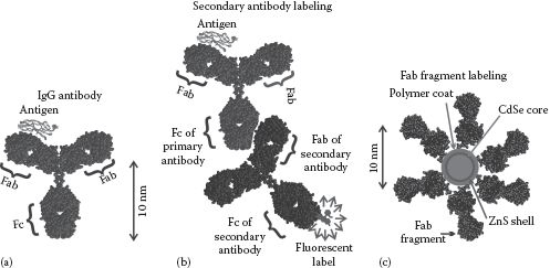
An antibody, or immunoglobulin (Ig), is a complex protein with bound sugar groups produced by cells of the immune system in animals to bind to specific harmful infecting agents in the body, such as bacteria and viruses. The basic structure of the most common class of antibody is Y-shaped (Figure 7.1), with a high molecular weight of ~150 kDa. The types (or isotypes) of antibodies of this class are mostly found in mammals and are IgD (found in milk/saliva), IgE (commonly produced in allergic responses), and IgG, which are produced in several immune responses and are the most widely used in biophysical techniques. Larger variants consisting of multiple Y-shaped subunits include IgA (a Y-subunit dimer) and IgM (a Y-subunit pentamer). Other antibodies include IgW (found in sharks and skates, structurally similar to IgD) and IgY (found in birds and reptiles).

Antibodies are also used significantly in single-molecule manipulation experiments. For example, single-molecule magnetic and optical tweezers experiments on DNA often utilize a label called “digoxigenin (DIG).” DIG is a steroid found exclusively in the flowers and leaves of the plants of the Digitalis genus, highly toxic to animals and perhaps as a result through evolution has highly immunogenic properties (meaning it has a high ability to provoke an immune response, thus provoking production of several specific antibodies to bind to DIG), and antibodies with specificity against DIG (called generally “anti-DIG”) have very high affinity. DIG is often added to one end of a DNA molecule, while a trapped bead that has been coated in anti-DIG molecule can then bind to it to enable single-molecule manipulation of the DNA.

DIG is an example of a class of chemical called “haptans.” These are the most common secondary labeling molecule for immuno-hybridization chemistry, due to their highly immunogenic properties (e.g., biotin is a haptan). DIG is also commonly used in fluorescence in situ hybridization (FISH) assays. In FISH, DIG is normally covalently bound to a specific nucleotide triphosphate probe, and the fluorescently labeled IgG secondary antibody anti-DIG is subsequently used to probe for its location on the chromosome, thus allowing specific DNA sequences, and genes, to be identified following fluorescence microscopy.

Click chemistry is the general term that describes chemical synthesis by joining small-molecule units together both quickly and reliably, which is ideally modular and has high yield. It is not a single specific chemical reaction. However, one of the most popular examples of click chemistry is the azide–alkyne Huisgen cycloaddition. This chemical reaction uses copper as a catalyst and results in a highly selective and strong covalent bond formed between azide (triple bonded N—N atoms) and alkyne (triple bonded C—C bonds) chemical groups to form stable 1,2,3-triazoles. This method of chemical conjugation is rapidly becoming popular in part due to its specific use in conjunction with increased development of oligonucleotide labeling.

Short ~10 base pair sequences of nucleotide bases known as oligonucleotides (or just oligos) can be used to label specific sites on a DNA molecule. A DNA sequence can be cut at specific locations by enzymes called “restriction endonucleases,” which enables short sequences of DNA complementary to a specific oligo sequence to be inserted at that location. Incubation with the oligo will then result in binding to the complementary sequence. This is useful since oligos can be modified to be bound to a variety of chemical groups, including biotin, azide, and alkynes, to facilitate conjugation to another biomolecule or structure. Also, oligos can be derivatized with a fluorescent dye label either directly or via, for example, a bound biotin molecule, to enable fluorescence imaging visualization of specific DNA sequence locations.

Aptamers are short sequences of either nucleotides or amino acids that bind to a specific region of a target biomolecule. These peptides and RNA- or DNA-based oligonucleotides have a molecular weight that is relatively low at ~8–25 kDa compared to antibodies that are an order of magnitude greater. Most aptamers are unnatural in being chemically synthesized structures, though some natural aptamers do exist, for example, a class of RNA structures known as riboswitches (a riboswitch is an interesting component of some mRNA molecules that can alter the activity of proteins that are involved in manufacturing the mRNA and so regulate their own activity).

Aptamers fold into specific 3D shapes to fit tightly to specific structural motifs for a range of different biomolecules with a very low unbinding rate measured as an equivalent dissociation constant in the pico- to nanomolar range. They operate solely via a structural recognition process, that is, no chemical bonding is involved. This is a similar process to that of an antigen–antibody reaction, and thus aptamers are also referred to as chemical antibodies.

Due to their relatively small size, aptamers offer some advantages over protein-based antibodies. For example, they can penetrate tissues faster. Also, aptamers in general do not evoke a significant immune response in the human body (they are described as nonimmunogenic). They are also relatively stable to heat, in that their tertiary and secondary structures can be denatured at temperatures as high as 95°C, but will then reversibly fold back into their original 3D conformation once the temperature is lowered to ~50°C or less, compared to antibodies that would irreversibly denature. This enables faster chemical reaction rates during incubation stages, for example, when labeling aptamers with fluorophore dye tags.

Aptamers can recognize a wide range of targets including small biomolecules such as ATP, ions, proteins, and sugars, but will also bind specifically to larger length scale biological matter, such as cells and viruses. The standard method of aptamer manufacture is known as systematic evolution of ligands by exponential enrichment. It involves repeated binding, selection, and then amplification of aptamers from an initial library of as many as ~10¹⁸ random sequences that, perhaps surprisingly, can home in on an ideal aptamer sequence in a relatively cost-effective manner.

Aptamers have significant potential for use as drugs, for example, to block the activity of a range of biomolecules. Also, they have been used in biophysical applications as markers of a range of biomolecules. For example, although protein metabolites can be labeled using fluorescent proteins, this is not true for nonprotein biomolecules. However, aptamers can enable such biomolecules to be labeled, for example, if chemically tagged with a fluorophore they can report on the spatial localization of ATP accurately in live cells using fluorescence microscopy techniques, which is difficult to quantify using other methods.

Technical advances of light microscopy have now enabled the capability to monitor whole, functional organisms (see Chapter 3). Biophysics here has gone full circle in this sense, from its earlier historical conception in, in essence, physiological dissection of relatively large masses of biological tissue. A key difference now however is one of enormously enhanced spatial and temporal resolution. Also, researchers now benefit greatly from a significant knowledge of underlying molecular biochemistry and genetics. Much progress has been made in biophysics through the experimental use of carefully selected model organisms that have ideal properties for light microscopy in particular; namely, they are thin and reasonably optically transparent. However, model organisms are also invaluable in offering the researcher a tractable biological system that is already well understood at a level of biochemistry and genetics.

There are a few select model bacteria species that have emerged as model organisms. Escherichia coli (E. coli) is the best known. E. coli is a model Gram-negative organism (see Chapter 2) whose genome (i.e., total collection of genes in each cell) comprises only ~4000 genes. There are several genetic variants of E. coli, noting that the spontaneous mutation rate of a nucleotide base pair in E. coli is ~10⁻⁹ per base pair per cell generation, some of which may generate a selective advantage for that individual cell and so be propagated to subsequent generations through natural selection (see Chapter 2). However, there are in fact only four key cell sources from which almost all of the variants are in use in modern microbiology research, which are called K-12, B, C, and W. Of these, K-12 is mostly used, which was originally isolated from the feces of a patient recovering from diphtheria in Stanford University Hospital in 1922.

Gram-positive bacteria lack a second outer cell membrane that Gram-negative bacteria possess. As a result, many exhibit different forms of biophysical and biochemical interactions with the outside world, necessitating a model Gram-positive bacterium for their study. The most popular model Gram-positive bacterium is currently Bacillus subtilis, which is a soil-dwelling bacterium. It undergoes an asymmetrical spore-forming process as part of its normal cell cycle, and this has been used as a mimic for biochemically triggered cell shape changes such as those that occur in higher organisms during the development of complex tissues.

There are many viruses known to infect bacteria, known as bacteriophages. Although, by the definition used in this book, viruses are not living as such, they are excellent model systems for studying genes. This is because they do not possess many genes (typically only a few tens of native genes), but rather hijack the genetic machinery of their host cell; if this host cell itself is a model organism such as E. coli, then this can offer significant insights into methods of gene operation/regulation and repair, for example. The most common model bacterium-infecting virus is called “bacteriophage lambda” (or just lambda phage) that infects E. coli. This has been used for many genetics investigations, and in fact since its DNA genetic code of almost ~49,000 nucleotide base pairs is so well characterized, methods for its reliable purification have been developed, and so there exists a readily available source of this DNA (called λ DNA), which is used in many in vitro investigations, including single-molecule experiments of optical and magnetic tweezers (see Chapter 6). Another model of bacterium-infecting virus includes bacteriophage Mu (also called Mu phage), which has generated significant insight into relatively large transposable sections of DNA called “transposons” that undergo a natural splicing out from their original location in the genetic code and relocated en masse in a different location.

Unlike prokaryotes, eukaryotes possess a distinct nucleus, as well as other subcellular organelles. This added compartmentalization of biological function can complicate experimental investigations (though note that even prokaryotes have distinct areas of local architecture in their cells so should not be perceived as a simple “living test tube”). Model eukaryotes for the study of cellular effects possess relatively few genes and also are ideally easy to cultivate in the laboratory with a reasonably short cell division time allowing cell cultures to be prepared quickly. In this regard, three organisms have emerged as model organisms. One includes the single-celled eukaryotic protozoan parasite of the Trypanosoma genus that causes African sleeping sickness, specifically a species called Trypanosoma brucei, which has emerged as a model cell to study the synthesis of lipids. A more widely used eukaryote model cell organism is yeast, especially the species called Saccharomyces cerevisiae also known as budding yeast or baker’s yeast. This has been used in multiple light microscopy investigations, for example, involving placing a fluorescent tag on specific proteins in the cell to perform superresolution microscopy (see Chapter 4). The third very popular model eukaryote unicellular organism is Chlamydomonas reinhardtii (C. reinhardtii). This is a green alga and has been used extensively to study photosynthesis and cell motility.

Dictyostelium discoideum is a more complex multicellular eukaryote, also known as slime mould. It has been used as a model organism in studies involving cell-to-cell communication and cell differentiation (i.e., how eukaryote cells in multicellular organisms commit to being different specific cell types). It has also been used to investigate the effects of programmed cell death, or apoptosis (see the following text).

More complex eukaryotic cells are those that would normally reside in tissues, and many biomedical investigations benefit from model human cells to perform investigations into human disease. The main problem with using more complex cells from animals is that they normally undergo the natural process of programmed cell death, called apoptosis, as part of their cell cycle. This means that it is impossible to study such cells over multiple generations and also technically challenging to grow a cell culture sample. To overcome this, immortalized cells are used, which have been modified to overcome apoptosis.

An immortal cell derived from a multicellular organism is one that under normal circumstances would not proliferate indefinitely but, due to being genetically modified, is no longer limited by the Hayflick limit. This is a limit to future cell division set either by DNA damage or by shortening of cellular structures called “telomeres,” which are repeating DNA sequences that cap the end of chromosomes (see Chapter 2). Telomeres normally get shorter with each subsequent cell division such that at a critical telomere length cell death is triggered by the complex biochemical and cellular process of apoptosis. However, immortal cells can continue undergoing cell division and be grown under cultured in vitro conditions for prolonged periods. This makes them invaluable for studying a variety of cell processes in complex animal cells, especially human cells.

Cancer cells are natural examples of immortal cells, but can also be prepared using biochemical methods. Common immortalized cell lines include the Chinese hamster ovary, human embryonic kidney, Jurkat (T lymphocyte, a cell type used in the immune response), and 3T3 (mouse fibroblasts from connective tissue) cells. However, the oldest and most commonly utilized human cell strain is the HeLa cell. These are epithelial cervical cells that were originally cultured from a cancerous cervical tumor of a patient named Henrietta Lacks in 1951. She ultimately died as a result of this cancer, but left a substantial scientific research legacy in these cells. Although there are potential limitations to their use in having undergone potentially several mutations from the original normal cell source, they are still invaluable to biomedical research utilizing biophysical techniques, especially those that use fluorescence microscopy.

Traditionally, plants have received less historical interest as the focus of biophysical investigations compared to animal studies, due in part to the lower relevance to human biomedicine. However, global issues relating to food and energy (see Chapter 9) have focused recent research efforts in this direction in particular. Many biophysical techniques have been applied to monitoring the development of complex plant tissues, especially involving advanced light microscopy techniques such as light sheet microscopy (see Chapter 4), which has been used to study the development of plant roots from the level of a few cells up to complex multicellular tissue.

The most popular model plant organism is Arabidopsis thaliana, also known commonly as mouse ear cress. It is a relatively small plant with a short generation time and thus easy to cultivate and has been characterized extensively genetically and biochemically. It was the first plant to have its full genome sequenced.

Two key model animal organisms for biophysics techniques are those that optimized for in vivo light microscopy investigations, including the zebrafish Danio rerio and the nematode flatworm Caenorhabditis elegans. The C. elegans flatworm is ~1 mm in length and ~80 μm in diameter, which lives naturally in soil. It is the simplest eukaryotic multicellular organism known to possess only ~1000 cells in its adult form. It also breeds relatively easily and fast taking ~3 days to reach maturation, which allows experiments to be performed reasonably quickly, is genetically very well characterized, and has many tissue systems that have generic similarities to those of other more complex organisms, including a complex network of nerves, blood vessels and heart, and a gut. D. rerio is more complex in having ~10⁶ cells in total in the adult form, and a length of a few cm and several hundred microns thick, and takes more like ~3 months to reach maturation.

These characteristics set more technical challenges on the use of D. rerio compared to C. elegans; however, it has a significant advantage in possessing a spinal cord in which C. elegans does not, making it the model organism of choice for investigating specifically vertebrate features, though C. elegans has been used in particular for studies of the nervous system. These investigations were first pioneered by the Nobel Laureate Sydney Brenner in the 1960s, but later involved the use of advanced biophysics optical imaging and stimulation methods using an invaluable technique of optogenetics, which can use light to control the expression of genes (see later in this chapter). At the time of writing, C. elegans is the only organism for which the connectome (the wiring diagram of all nerve cells in an organism) has been determined.

The relative optical transparency of these organisms allows standard bright-field light microscopy to be performed, a caveat being that adult zebrafish grow pigmented stripes on their skin, hence their name, which can impair the passage of visible light photons. However, mutated variants of zebrafish have now been produced in which the adult is colorless.

Among invertebrate organisms, that is, those lacking an internal skeleton, Drosophila melanogaster (the common fruit fly) is the best studied. Fruit flies are relatively easy to cultivate in the laboratory and breed rapidly with relatively short life cycles. They also possess relatively few chromosomes and so have formed the basis of several genetics studies, with light microscopy techniques used to identify positions of specifically labeled genes on isolated chromosomes.

For studying more complex biological processes in animals, rodents, in particular mice, have been an invaluable model organism. Mice have been used in several biophysical investigations involving deep tissue imaging in particular. Biological questions involving practical human biomedicine issues, for example, the development of new drugs and/or investigating specific effects of human disease that affects multiple cell types and/or multiply connected cells in tissues, ultimately involve larger animals of greater similarity to humans, culminating in the use of primates. The use of primates in scientific research is clearly a challenging issue for many, though such investigations require significant oversight before being granted approval from ethical review committees that are independent from the researchers performing the investigations.

Multiple biophysical investigations requiring tractable, well-characterized organism systems to study a range of biological processes.

KEY POINT 7.3

A “model organism,” in terms of the requirements for biologists, is selected on its being genetically and phenotypically/behaviorally very well characterized from previous experimental studies and also possesses biological features that at some level are “generic” in allowing us to gain insight into a biological process common to many organisms (especially true for biological processes in humans, since these give us potential biomedical insight). For the biophysicist, these organisms must also satisfy an essential condition of being experimentally very tractable. For animal tissue research, this includes the use of thin, optically transparent organisms for light microscopy. One must always bear in mind that some of the results from model organisms may differ in important ways from other specific organisms that possess equivalent biological processes under study.

The ability to sequence and then controllably modify the DNA genetic code of cells has complemented experimental biophysical techniques enormously. These genetic technologies enable controlled expression of specific proteins for purification and subsequent in vitro experimentation as well as enable the study of the function of specific genes by modifying them through controlled mutation or deleting them entirely, such that the biological function might be characterized using a range of biophysical tools discussed in the previous experimental chapters of this book. One of the most beneficial aspects of this modern molecular biology technology has been the ability to engineer specific biophysical labels at the level of the genetic code, through incorporation either of label binding sites or of fluorescent protein sequences directly.

Molecular cloning describes a suite of tools using a combination of genetic engineering, cell and molecular biology, and biochemistry, to generate modified DNA, to enable it to be replicated within a host organism (“cloning” simply refers to generating a population of cells all containing the same DNA genetic code). The modified DNA may be derived from the same or different species as the host organism.

In essence, for cloning of genomic DNA (i.e., DNA obtained from a cell’s nucleus), the source DNA, which is to be modified and ultimately cloned, is first isolated and purified from its originator species. Any tissue/cell source can in principle be used for this provided the DNA is mostly intact. This DNA is purified (using a phenol extraction), and the number of purified DNA molecules present is amplified using polymerase chain reaction (PCR) (see Chapter 2). To ensure efficient PCR, primers need to be added to the DNA sequence (short sequences of 10–20 nucleotide base pairs that act as binding sites for initiating DNA replication by the enzyme DNA polymerase). PCR can also be used on an RNA sample sources, but using a modified PCR technique of the reverse transcription polymerase chain reaction that first converts RNA back into complementary DNA (cDNA) that is then amplified using conventional PCR. A similar process can also be used on synthetic DNA, that is, artificial DNA sequences not from a native cell or tissue source.

The amplified, purified DNA is then chemically broken up into fragments by restriction endonuclease enzymes, which cut the DNA at specific sequence locations. At this stage, additional small segments of DNA from other sources may be added that are designed to bind to specific cut ends of the DNA fragments. These modified fragments are then combined with vector DNA. In molecular biology, a vector is a DNA molecule that is used to carry modified (often foreign) DNA into a host cell, where it will ultimately be replicated and the genes in that recombinant DNA expressed can be replicated and/or expressed. Vectors are generally variants of either bacterial plasmids or viruses (see Chapter 2). Such a vector that contains the modified DNA is known as recombinant DNA. Vectors in general are designed to have multiple specific sequence restriction sites that recognize the corresponding fragment ends (called “sticky ends”) of the DNA generated by the cutting action of the restriction endonucleases. Another enzyme called “DNA ligase” catalyzes the binding of the sticky ends into the vector DNA at the appropriate restriction site in the vector, in a process called ligation. It is possible for other ligation products to form at this stage in addition to the desired recombinant DNA, but these can be isolated out at a later stage after the recombinant DNA has been inserted in the host cell.

Insertion of the recombinant DNA into the target host cell is done through a process called either “transformation” for bacterial cells, “transfection” for eukaryotic cells, or, if a virus is used as a vector, “transduction” (the term “transformation” in the context of animal cells actually refers to changing to a cancerous state, so is avoided here). The recombinant DNA needs to pass through the cell membrane barrier, and this can be achieved using both natural and artificial means. For natural transformation to occur, the cell must be in a specific physiological state, termed competent, which requires the expression of typically tens of different proteins in bacteria to allow the cell to take up and incorporate external DNA from solution (e.g., filamentous pili structures of the outer member, as well as protein complexes in the cell membrane to pump DNA from the outside to the inside). This natural phenomenon in bacteria occurs in a process called “horizontal gene transfer,” which results in genetic diversity through transfer of plasmid DNA between different cells, and is, for example, a mechanism for propagating antibiotic resistance in a cell population. It may also have evolved as a mechanism to assist in the repair of damaged DNA, that is, to enable the internalization of nondamaged DNA that can then be used as a template from which to repair native damaged DNA.

Artificial methods can improve the rate of transformation. These can include treating cells first with enzymes to strip away outer cells walls, adding divalent metal ions such as magnesium or calcium to increase binding of DNA (which has a net negative charge in solution due to the presence of the backbone of negatively charged phosphate groups), or increasing cell membrane fluidity. These also include methods that involve a combination of cold and heat shocking cells to increase internalization of recombinant by undetermined mechanisms as well as using ultrasound (sonication) to increase the collision frequency of recombinant DNA with host cells. The most effective method however is electroporation. This involves placing the aqueous suspension of host cells and recombinant DNA into an electrostatic field of strength 10–20 kV cm⁻¹ for a few milliseconds that increases the cell membrane permeability dramatically through creating transient holes in the membrane through which plasmid DNA may enter.

Transfection can be accomplished using an extensive range of techniques, some of which are similar to those used for transformation, for example, the use of electroporation. Other more involved methods have been optimized specifically for host animal cell transfection however. These include biochemical-based methods such as packaging recombinant DNA into modified liposomes that then empty their contents into a cell upon impact on, and merging with, the cell membrane. A related method is protoplast fusion that involves chemically or enzymatically stripping away the cell wall from a bacterial cell to enable it to fuse in suspension with a host animal cell. This delivers the vector that may be inside the bacterial cell, but with the disadvantage of delivery of the entire bacterial cell contents, which may potentially be detrimental to the host cell.

But there are also several biophysical techniques for transfection. These include sonoporation (using ultrasound to generate transient pores in cell membranes), cell squeezing (gently massaging cells through narrow flow channels to increase the membrane permeability), impalefection (introducing DNA bound to a surface of a nanofiber by stabbing the cell), gene guns (similar to impalefection but using DNA bound to nanoparticles that are fired into the host cell), and magnet-assisted transfection or magnetofection (similar to the gene gun approach, though here DNA is bound to a magnetic nanoparticle with an external B-field used to force the particles into the host cells).

The biophysical transfection tool with the most finesse involves optical transfection, also known as photoporation. Here, a laser beam is controllably focused onto the cell membrane generating localized heating sufficient to form a pore in the cell membrane and allow recombinant DNA outside the cell to enter by diffusion. Single-photon absorption processes in the lipid bilayer can be used here, centered on short wavelength visible light lasers; however, better spatial precision is enabled by using a high-power near-infrared (IR) femtosecond pulsed laser that relies on two-photon absorption in the cell membrane, resulting in smaller pores and less potential cell damage.

Viruses undergoing transfection (i.e., viral transduction) are valuable because they can transfer genes into a wide variety of human cells in particular with very high transfer rates. However, this method can also be used for other cell types, including bacteria. Here, the recombinant DNA is packaged into an empty virus capsid protein coat (see Chapter 2). The virus then performs its normal roles of attaching to host cell and then injecting the DNA into the cell very efficiently, compared to the other transfection/transformation methods.

The process of inserting recombinant DNA into a host cell has normally low efficiency, with only a small proportion of host cells successfully taking up the external DNA. This presents a technical challenge in knowing which cells have done so, since these are the ones that need to be selectively cultivated from a population. This selection is achieved by engineering one or more selectable markers into the vector. A selectable marker is usually a gene conferring resistance against a specific antibiotic that would otherwise be lethal to the cell. For example, in bacteria, there are several resistance genes available that are effective against broad-spectrum antibiotics such as ampicillin, chloramphenicol, and kanamycin. Those host cells that have successfully taken up a plasmid vector during transformation will survive culturing conditions that include the appropriate antibiotic, whereas those that have not taken up the plasmid vector will die. Using host animal cells, such as human cells, involves a similar strategy to engineer a stable transfection such that the recombinant DNA is incorporated ultimately into the genomic DNA, using a marker gene that is encoded into the genomic DNA conferring resistance against the antibiotic Geneticin. Unstable or transient transfection does not utilize marker genes on the host cell genome but instead retains the recombinant DNA as plasmids. These ultimately become diluted after multiple cell generations and so the recombinant DNA is lost.

SDM is a molecular biology tool that uses the techniques of molecular cloning described earlier to make controlled, spatially localized mutations to a DNA sequence, at the level of just a few, or sometimes one, nucleotide base pairs. The types of mutations include a single base change (point mutation), deletion or insertion, as well as multiple base pair changes. The basic method of SDM uses a short DNA primer sequence that contains the desired mutations and is complementary to the template DNA around the mutation site and can therefore displace the native DNA by hybridizing with the DNA in forming stable Watson–Crick base pairs. This recombinant DNA is then cloned using the same procedure as described in Section 7.4.

SDM has been used in particular to generate specific cysteine point mutations. These have been applied for bioconjugation of proteins as already discussed in the chapter and also for a technique called cysteine scanning (or cys-scanning) mutagenesis. In cys-canning mutagenesis, multiple point mutations are made to generate several foreign cysteine sites, typically in pairs. The purpose here is that if a pair of such nonnative cysteine amino acids is biochemically detected as forming a disulphide bond in the resultant protein, then this indicates that these native residue sites that were mutated must be within ~0.2 nm distance. In other words, it enables 3D mapping of the location of different key residues in a protein. This was used, for example, in determining key residues used in the rotation of the F1Fo-ATP synthase that generates the universal cellular fuel of ATP (see Chapter 2).

A similar SDM technique is that of alanine scanning. Here, the DNA sequence is point mutated to replace specific amino acid residues in a protein with the amino acid alanine. Alanine consists of just a methyl (—CH₃) substituent group and so exhibits relatively little steric hindrance effects, as well as minimal chemical reactivity. Substituting individual native amino acid residues with alanine, and then performing a function test on that protein, can generate insight into the importance of specific amino acid side groups on the protein’s biological function.

There are several molecular biology tools that allow control of the level of protein expression from a gene. The ultimate control is to delete the entire gene from the genome of a specific population of cells under investigation. These deletion mutants, also known as gene knockouts, are often invaluable in determining the biological function of a given gene, since the mutated cells can be subjected to a range of functionality tests and compares against the native cell (referred to as the wild type).

A more finely tuned, reversible method to modify gene expression is to use RNA silencing. RNA silencing is a natural and ubiquitous phenomenon in all eukaryote cells in which the expression of one or more genes is downregulated (which in molecular biology speaks for “lowered”) or turned off entirely by the action of a small RNA molecule whose sequence is complementary to a region of an mRNA molecule (which would ultimately be translated to a specific peptide or protein). RNA silencing can be adapted by generating synthetic small RNA sequences to specially and controllably regulate gene expression. Most known RNA silencing effects operate through such RNA interference, using either microRNA or similar small interfering RNA molecules, which operate via subtly different mechanisms but which both ultimately result in the degradation of a targeted mRNA molecule.

Gene expression in prokaryotes can also be silenced using a recently developed technique that utilizes clustered regularly interspaced short palindromic repeats (CRISPR, pronounced “crisper,” Jinek et al., 2012). CRISPR-associated genes naturally express proteins whose biological role is to catalyze the fragmentation of external foreign DNA and insert them into these repeating CRISPR sequences on the host cell genome. When these small CRISPR DNA inserts are transcribed into mRNA, they silence expression of the external DNA—it is a remarkable bacterial immune response against invading pathogens such as viruses. However, the CRISPR are also found in several species that are used as model organisms including C. elegans and zebrafish and can also be effective in human cells as a gene silencing tool. CRISPR has enormous potential for revolutionizing the process of gene editing.

Transcription activator-like effector nucleases (TALENs) can also be used to suppress expression from specific to genes. TALENs are enzymes that could be encoded onto a plasmid vector in a host cell. These can bind to a specific sequence of DNA and catalyze cutting of the DNA at that point. The cell has complex enzyme systems to repair such a cut DNA molecule; however, the repaired DNA is often not a perfect replica of the original that can result in a nonfunctional protein expressed from this repaired DNA. Thus, although gene expression remains there is no functional protein which results.

RNA silencing can also use upregulated (i.e., “increased”) gene expression, for example, by silencing a gene that expresses a transcription factor (see Chapter 2) that would normally represses the expression of another gene. Another method to increase gene expression includes concatemerization of genes, that is, generating multiple sequential copies under control of the same promoter (see Chapter 2).

Expression of genes in plasmids, especially those in bacteria, can be controlled through inducer chemicals. These chemicals affect the ability of a transcription factor to bind to a specific promoter of an operon. The operon is a cluster of genes on the same section of the chromosome that are all under control of the same promoter, all of which get transcribed and translated in the same continuous gene expression burst (see Chapter 2). The short nucleotide base pair sequence of the promoter on the DNA acts as an initial binding site for RNA polymerase and determines where transcription of an mRNA sequence translated from the DNA begins. Insight into the operation of this system was made originally using studies of the bacterial lac operon, and this system is also used today to control gene expression of recombinant DNA in plasmids.

Although some transcription factors act to recruit the RNA polymerase, and so result in upregulation, most act as repressors through binding to the promoter that inhibits binding of RNA polymerase, as is the case in the lac operon. The lac operon consists of three genes that express enzymes involved in the internalization into the cell and metabolism of the disaccharide lactose into the monosaccharides glucose and galactose. Decreases in the cell’s concentration of lactose result in reduced affinity of the repressor protein to the lacI gene that in turn is responsible for generating the LacI protein repressor molecule that inhibits expression of the operon genes and is by default normally switched “on” (note that the names of genes are conventionally written in italics starting with a lowercase letter, while the corresponding protein, which is ultimately generated from that gene following transcription and translation, is written in non-italics using the same word but with the first letter in uppercase). This prevents operon gene expression. This system is also regulated in the opposite direction by a protein called CAP whose binding in the promoter region is inversely proportional to cellular glucose concentration. Thus, there is negative feedback between gene expression and the products of gene expression.

The nonnative chemical isopropyl-β-D-thio-galactoside (IPTG) binds to LacI and in doing so reduces the Lacl affinity to the promoter, thus causing the operon genes to be expressed. This effect is used in genetic studies involving controllable gene expression in bacteria. Here, a gene under investigation desired to be expressed is fused upstream of the lac promoter region in the lac operon and into a plasmid vector using the molecular cloning methods described earlier in this chapter. These plasmids are also replicated during normal cell growth and division and so get passed on to subsequent cell generations.

If IPTG is added to the growth media, it will be ingested by the cells, and the repressing effects of LacI will be inactivated; thus, the protein of interest will start to be made by the cells, often at levels far above normal wild type levels, as it is difficult to prevent a large number of plasmids from being present in each cell. Since IPTG does not have an infinite binding affinity to LacI, there is still some degree of suppression of protein production, but also the LacI repressor similarly is not permanently bound to the operator region, and so if even in the absence of IPTG, a small amount of protein is often produced (this effect is commonly described as being due to a leaky plasmid).

In theory, it is possible to cater the IPTG concentration to a desired cellular concentration of expressed protein. In practice though the response curve for changes in IPTG concentration is steeply sigmoidal, the effect is largely all or nothing in response to changes in IPTG concentration. However, another operon system used for genetics research in E. coli and other bacteria is the arabinose operon that uses the monosaccharide arabinose as the equivalent repressor binder; here the steepness of the sigmoidal response is less than the IPTG operon system, which makes it feasible to control the protein output by varying the external concentration of arabinose.

A valuable technique for degrading the activity of specific expressed proteins from genes in prokaryotes is degron-targeted proteolysis. Prokaryotes have a native system for reducing the concentration level of specific proteins in live cells, which involves their controlled degradation by proteolysis. In the native cell, proteins are first marked for degradation by tagging them with a short amino acid degradation sequence, or degron. In E. coli, an adaptor protein called SspB facilitates binding of protein substrates tagged with the SsrA peptide to a protease called “ClpXP” (pronounced “Clip X P”). ClpXP is an enzyme that specifically leads to proteolytic degradation of proteins that possess the degron tag.

This system can be utilized synthetically by using molecular cloning techniques to engineer a foreign ssrA tag onto a specific protein which one wishes to target for degradation. This modification is then transformed into a modified E. coli cell strain in which the native gene sspB that encodes for the protein SspB has been deleted. Then, a plasmid that contains the sspB gene is transformed into this strain such that expression of this gene is under control on an inducible promoter. For example, this gene might then be switched “on” by the addition of extracellular arabinose to an arabinose-inducible promoter, in which case the SsrB protein is manufactured that then results in proteolysis of the SsrA-tagged protein.

This is a particularly powerful approach in the case of studying essential proteins. An essential protein is required for the cell to function, and so deleting the protein would normally be lethal and no cell population could be grown. However, by using this degron-tagging strategy, a cell population can first be grown in the absence of SspB expression, and these cells are then observed following controlled degradation of the essential protein after arabinose (or equivalent) induction.

As outlined previously, several options exist for fluorescent tags to be encoded into the DNA genetic code of an organism, either directly, in the case of fluorescent proteins, or indirectly, in the case of SNAP/CLIP-tags. Similarly, different segment halves of a fluorescent protein can be separately encoded next to the gene that expresses proteins that are thought to interact, in the BiFC technique, which generates a functional fluorescent protein molecule when two such proteins are within a few nm distance (see Chapter 3).

Most genetically encoded tags are engineered to be at one of the ends of the protein under investigation, to minimize structural disruption of the protein molecule. Normally, a linker sequence is used of ~10 amino acids to increase the flexibility with the protein tag and reduce steric hindrance effects. A common linker sequence involves repeats of the amino acid sequence “EAAAK” bounded by alanine residues, which is known to form stable but flexible helical structures (whose structure resembles a conventional mechanical spring). The choice of whether to use the C- or N-terminus of a protein is often based on the need for binding at or near to either terminus as part of the protein’s biological function, that is, a terminus is selected for tagging so as to minimize any disruption to the normal binding activities of the protein molecule. Often there may be binding sequences at both termini, in which case the binding ability can still be retained in the tagged sequence by copying the end DNA sequence of the tagged terminus onto the very end of the tag itself.

Ideally, the native gene for a protein under investigation is entirely deleted and replaced at the same location in the DNA sequence by the tagged gene. However, sometimes this results in too significant an impairment of the biological function of the tagged protein, due to a combination of the tag’s size and interference of native binding surfaces of the protein. A compromise in this circumstance is to retain the native untagged gene on the cell’s genome but then create an additional tagged copy of the gene on a separate plasmid, resulting in a merodiploid strain (a cell strain that contains a partial copy of its genome). The disadvantage with such techniques is that there is a mixed population of tagged and untagged protein in the cell, whose relative proportion is often difficult to quantify accurately using biochemical methods such as western blots (see Chapter 6).

A useful tool for researchers utilizing fluorescent proteins in live cells is the ASKA library (Kitagawa et al., 2005), which stands for “A complete Set of E. coli K-12 ORF Archive.” It is a collection (or “library”) of genes fused to genetically encoded fluorescent protein tags. Here, each open reading frame (or “ORF”), that is, the region of DNA between adjacent start and stop codons that contains one or more genes (see Chapter 2), in the model bacterium E. coli, has been fused with the DNA sequence for the yellow variant of GFP, YFP. The library is stored in the form of DNA plasmid vectors under IPTG inducer control of the lac operon.

In principle, each protein product from all coding bacterial genes is available to study using fluorescence microscopy. The principle weakness with the AKSA library is that the resultant protein fusions are all expressed at cellular levels that are far more concentrated than those found for the native nonfusion protein due to the nature of the IPTC expression system employed, which may result in nonphysiological behavior. However, plasmid construct sequences can be spliced out from the ASKA library and used for developing genomically tagged variants.

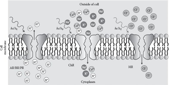
Optogenetics (see Pastrana, 2010; Yizhar et al., 2011) specifically describes a set of techniques that utilize light-sensitive proteins that are synthetically genetically coded into nerve cells. These foreign proteins are introduced into nerve cells using the transfection delivery methods of molecular cloning described earlier in this chapter. These optogenetics techniques enable investigation into the behavior of nerves and nerve tissue by controlling the ion flux into and out of a nerve cell by using localized exposure to specific wavelengths of visible light. Optogenetics can thus be used with several advanced light microscopy techniques, especially those of relevance to deep tissue imaging such as multiphoton excitation methods (see Chapter 4). These light-sensitive proteins include a range of opsin proteins (referred to as luminopsins) that are prevalent in the cell membranes of single-celled organisms as channel protein complexes. These can pump protons, or a variety of other ions, across the membrane using the energy from the absorption of photons of visible light, as well as other membrane proteins that act as ion and voltage sensors (Figure 7.2).

Similarly halorhodopsin is a chloride ion pump found in a type of archaea known as halobacteria that thrive in very salty conditions, whose biological role is to maintain the osmotic balance of a cell by pumping chloride into their cytoplasm from the outside, energized by absorption of yellow/green light (typically 540 nm < λ < 590 nm). Channelrhodopsin (ChR), which is found in the single-celled model alga C. reinhardtii, acts as a pump for a range of nonspecific positive ions including protons, Na⁺ and K⁺ as well as the divalent Ca²⁺ ion. However, here longer wavelength red light (λ > 590 nm) fuels a pumping action from the outside of the cell to the cytoplasm inside.

In addition, light-sensitive protein sensors are used, for example, chloride and calcium ion sensors, as well as membrane voltage sensor protein complexes. Finally, another class of light-sensitive membrane integrated proteins are used, the most commonly used being the optoXR type. These undergo conformational changes upon the absorption of light, which triggers intracellular chemical signaling reactions.

The light-sensitive pumps used in optogenetics have a typical “on time” constant of a few ms, though this is dependent on the local excitation of laser illumination. The importance of this is that it is comparable to the electrical conduction time from one end of a single nerve cell to the other and so in principle allows individual action potential pulses to be probed. The nervous conduction speed varies with nerve cell type but is roughly in the range 1–100 ms⁻¹, and so a signal propagation time in a long nerve cell that is a few mm in length can be as slow as a few ms.

The “off time” constant, that is, a measure of either the time taken to switch from “on” to “off” following removal of the light stimulation, varies usually from a few ms up to several hundred ms. Some ChR complexes have a bistable modulation capability, in that they can be activated with one wavelength of light and deactivated with another. For example, ChR2-step function opsins (SFOs) are activated by blue light of peak λ = 470 nm and deactivated with orange/red light of peak λ = 590 nm, while a different version of this bistable ChR called VChR1-SFOs has the opposite dependence with wavelength such that it is activated by yellow light of peak λ = 560 nm, but deactivated with a violet light of peak λ = 390 nm. The off times for these bistable complexes are typically a few seconds to tens of seconds. Light-sensitive biochemical modulation complexes such as the optoXRs have off times of typically a few seconds to tens of seconds.

Genetic mutation of all light-sensitive protein complexes can generate much longer off times of several minutes if required. This can result in a far more stable on state. The rapid on times of these complexes enable fast activation to be performed either to stimulate nervous signal conduction in a single nerve cell or to inhibit it. Expanding the off time scale using genetic mutants of these lightsensitive proteins enables experiments using a far wider measurement sample window. Note also that since different classes of light-sensitive proteins operate over different regions of the visible light spectrum, this offers the possibility for combining multiple different light-sensitive proteins in the same cell. Multicolor activation/deactivation of optogenetics constructs in this way result in a valuable neuroengineering toolbox.

Optogenetics is very useful when used in conjunction with the advanced optical techniques discussed previously (Chapter 4), in enabling control of the sensory state of single nerve cells. The real potency of this method is that it spans multiple length scales of the nervous sensory system of animal biology. For example, it can be applied to individual nerve cells cultured from samples of live nerve tissue (i.e., ex vivo), to probe the effects of sensory communication between individual nerve cells. With advanced fluorescence microscopy methods, these can be combined with detection of single-molecule chemical transmitters at the synapse junctions between nerve cells, to explore the molecular scale mechanisms of sensory nervous conduction and regulation. But larger length scale experiments can also be applied using intact living animals to explore the ways that neural processing between multiple nerve cells occurs. For example, using light stimulation of optogenetically engineered parts of the nerve tissue in C. elegans can result in control of the swimming behavior of the whole organism. Similar approaches have been applied to monitor neural processing in fruit flies, and also experiments on live rodents and primates using optical fiber activation of optogenetics constructs in the brain have been performed to monitor the effect on whole organism movement and other aspects of animal behavior relating to complex neural processing. In other words, optogenetics enables insight into the operation of nerves from the length scale of single molecules through to cells and tissues up to the level of whole organisms. Such techniques have also a direct biomedical relevance in offering insights into various neurological diseases and psychiatric disorders.

Controlled gene expression investigations; Protein purification; Genetics studies.

Enormous advances have been made in the life sciences due to structural information of biomolecules, which is precise within the diameter of single constituent atoms (see Chapter 5). The most successful biophysical technique to achieve this, as measured by the number of different uploaded PDB files of atomic spatial coordinates of various biomolecule structures into the primary international PDB data repository of the Protein Data Bank (www.pdb.org, see Chapter 2), has been x-ray crystallography. We explored aspects of the physics of this technique previously in Chapter 5. At present, a technical hurdle in x-ray crystallography is the preparation of crystals that are large enough to generate a strong signal in the diffraction pattern while being of sufficient quality to achieve this diffraction to a high measurable spatial resolution. There are therefore important aspects to the practical methods for generating biomolecular crystals, which we discuss here.

The first step in making biomolecule crystals is to purify the biomolecule in question. Crystal manufacture ultimately requires a supersaturated solution of the biomolecule (meaning a solution whose effective concentration is above the saturation concentration level equivalent to the concentration in which any further increase in concentration results in biomolecules precipitating out of solution). This implies generating high concentrations equivalent in practice to several mg mL⁻¹.

Although crystals can be formed from a range of biomolecule types, including sugars and nucleic acids, the majority of biomolecule crystal structures that have been determined relate to proteins, or proteins interacting with another biomolecule type. The high purity and concentration required ideally utilizes molecular cloning of the gene coding for the protein in a plasmid to overexpress the protein. However, often a suitable recombinant DNA expression system is technically too difficult to achieve, requiring less ideal purification of the protein from its native cell/tissue source. This requires a careful selection of the best model organism system to use to maximize the yield of protein purified. Often bacterial or yeast systems are used since they are easy to grow in liquid cultures; however, the quantities of protein required often necessitate the growth of several hundred liters of cells in culture.

The methods used for extraction of biomolecules from the native source are classical biochemical purification techniques, for example, tissue homogenization, followed by a series of fractionation precipitation stages. Fractionation precipitation involves altering the solubility of the biomolecule, most usually a protein, by changing the pH and ionic strength of the buffer solution. The ionic strength is often adjusted by addition of ammonium sulfate at high concentrations of ~2.0 M, such that above certain threshold levels of ammonium sulfate, a given protein at a certain pH will precipitate out of a solution, and so this procedure is also referred to as ammonium sulfate precipitation.

At low concentrations of ammonium sulfate, the solubility of a protein actually increases with increasing ammonium sulfate, a process called “salting in” involving an increase in the number of electrostatic bonds formed between surface electrostatic amino acid groups and water molecules mediated through ionic salt bridges. At high levels of ammonium sulfate, the electrostatic amino acid surface residues will all eventually be fully occupied with salt bridges and any extra added ammonium sulfate results in attraction of water molecules away from the protein, thus reducing its solubility, known as salting out. Different proteins salt in and out at different threshold concentrations of ammonium sulfate; thus, a mixture of different proteins can be separated by centrifuging the sample to generate a pellet of the precipitated protein(s) and then subject either the pellet or the suspension to further biochemical processing—for example, to use gel filtration chromatography to further separate any remaining mixtures of biomolecules on the basis of size, shape, and charge, etc., in addition to methods of dialysis (see Chapter 6). Ammonium sulfate can also be used in the final stage of this procedure to generate a high concentration of the purified protein, for example, to salt out, then resuspend the protein, and dissolve fully in the final desired pH buffer for the purified protein to be crystallized. Other precipitants aside from ammonium sulfate can be used depending on the pH buffer and protein, including formate, ammonium phosphate, the alcohol 2-propanol, and the polymer polyethylene glycol (PEG) in a range of molecular weight value from 400 to 8000 Da.

Biomolecule crystallization, most typically involving proteins, is a special case of a thermodynamic phase separation in a nonideal mixture. Protein molecules separate from water in solution to form a distinct, ordered crystalline phase. The nonideal properties can be modeled as a virial expansion (see Equation 4.25) in which the parameter B is the second virial coefficient and is negative, indicative of net attractive forces between the protein molecules.

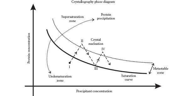
Once a highly purified biomolecule solution has been prepared, then in principle the attractive forces between the biomolecules can result in crystal formation if a supersaturated solution in generated. It is valuable to depict the dependence of protein solubility on precipitant concentration as a 2D phase diagram (Figure 7.3). The undersaturation zone indicates solubilized protein, whereas regions to the upper right of the saturation curve indicate the supersaturation zone in which there is more protein present than can be dissolved in the water available.

The crystallization process involves local decrease in entropy S due to an increase in the order of the constituent molecules of the crystals, which is offset by a greater increase in local disorder of all of the surrounding water molecules due to breakage of solvation bonds with the molecules that undergo crystallization. Dissolving a crystal breaks strong molecular bonds and so releases enthalpy H as heat (i.e., an exothermic process), and similarly crystal formation is an endothermic process. Thus, we can say that

Indeed, the trick for obtaining homogeneous crystals as opposed to amorphous precipitated protein is to span the metastable zone between supersaturation and undersaturation by making gradual changes to the effective precipitant concentration. For example, crystals can be simply formed using a solvent evaporation method, which results in very gradual increases in precipitant concentration due to the evaporation of solvent (usually water) from the solution. Other popular methods include slow cooling of the saturated solution, convection heat flow in the sample, and sublimation methods under vacuum. The most common techniques however are vapor diffusion methods.

Two popular types of vapor diffusion techniques used are sitting drop and hanging drop methods. In both methods, a solution of precipitant and concentrated but undersaturated protein is present in a droplet inside a closed microwell chamber. The chamber also contains a larger reservoir consisting of a precipitant at higher concentration than the droplet but no protein, and the two methods only essentially differ in the orientation of the protein droplet relative to the reservoir (in the hanging drop method the droplet is directly above the reservoir, in the sitting drop method it is shifted to the side). Water evaporated from the droplet is absorbed into the reservoir, resulting in a gradual increase in the protein concentration of the droplet, ultimately to supersaturation levels.

The physical principles of these crystallization methods are all similar; in terms of the phase diagram, a typical initial position in the crystallization process is indicated by point I on the phase diagram. Then, due to water evaporation from the solution, the position of the phase diagram will translate gradually to point II in the supersaturation zone just above the metastable zone. If the temperature and pH conditions are optimal, then a crystal may nucleate at this point. Further evaporation causes crystal growth and translation on the phase diagram to point III on the saturation curve. At this point, any further water evaporation then potentially results in translation back up the phase transition boundary curve to the supersaturation point IV, which again may result in further crystal nucleation and additional crystal growth. Nucleation may also be seeded by particulate contaminants in the solution, which ultimately results in multiple nucleation sites with each resultant crystal being smaller than were a single nucleation site present. Thus, solution and sample vessel cleanliness are also essential in generating large crystals. Similarly, mechanical vibration and air disturbances can result in detrimental multiple nucleation sites. But the rule of thumb with crystal formation is that any changes to physical and chemical conditions in seeding and growing crystals should be made slowly—although some proteins can crystallize after only a few minutes, most research grade protein crystals require several months to grow, sometimes over a year.

Nucleation can be modeled as two processes of primary nucleation and secondary nucleation. Primary nucleation is the initial formation such that no other crystals influence the process (because either they are not present or they are too far away). The rate B of primary nucleation can be modeled empirically as

n is an empirically determined exponent typically in the range 3–4, though it can be as high as ~10

The secondary nucleation process is more complex and is dependent on the presence of other nearby crystal nuclei whose separation is small enough to influence the kinetics of further crystal growth. Effects such as fluid shear are important here, as are collisions between preexisting crystals. This process can be modeled empirically as

j and b are empirical exponents of ~1 (as high as ~1.5) and ~2 (as high as ~5), respectively

Analytical modeling of the nucleation process can be done by considering the typical free energy change per molecule ΔG_n associated with nucleation. This is given by the sum of the bulk solution (ΔG_b) and crystal surface (ΔG_s) terms:

α is the interfacial free energy per unit area of a crystal of effective radius r

Δμ is the change in chemical potential of the crystallizing molecules, which measures the mean free energy change in a molecule transferring from the solution phase to the crystal phase

where σ is often called the “saturation.” Inspection of Equation 7.4 indicates that there is a local maximum in ΔG_n equivalent to the free energy barrier ΔG^* for nucleation at a particular threshold value of r known as the critical radius r_c:

In practice, two interfacial energies often need to be considered, one between the crystal and the solid substrate and the other between the crystal and the solid surface substrate in which crystals typically form on. Either way, substituting r_c into Equation 7.5 indicates

Thus the rate of nucleation J_n can be estimated from the equivalent Boltzmann factor:

where A and B are constants. Thus, there is a very sensitive dependence on nucleation rate with both the interfacial energy and the supersaturation. This is a key thermodynamic explanation for why the process of crystal formation is so sensitive to environmental conditions and is considered by some to be tantamount to a black art! Similar thermodynamic arguments can be applied to model the actual geometrical shape of crystals formed.

Many functional biomolecular complexes may be formed from multiple separate components. Obtaining crystals from these is harder since it requires not only a mixture of highly pure separate components but also one in which the relative stoichiometry of the components to each other is tightly constrained. Finding optimum temperature and pH conditions that avoid premature precipitation in the separate components is a key challenge often requiring significant experimental optimization. The use of microorganisms such as bacteria and unicellular eukaryotes to grow such crystals has shown recent promise, since the small volume of these cells can result in very concentrated intracellular protein concentration. Crystals for viral capsids (see Chapter 2) have been generated in this way, with the caveat that the crystal size will be limited to just a few microns length due to the small size of the cells used.

The precision of an x-ray crystal diffraction pattern is affected significantly by the homogeneity of the crystal, and its size. Controlled, gradual dehydration of crystals can result in an ultimate increase in crystal size, for example, using elevated concentration levels of PEG to draw out the water content, which in some cases can alter the shape of the crystal unit cell resulting in more efficient packing in a larger crystal structure. Also, small seed crystals placed in the undersaturated solution can be efficient sites for nucleation of larger growing larger crystals.

The use of crystallization robots has significantly improved the high-throughput nature of crystallization. These devices utilize vapor diffusion methods to automate the process of generating multiple crystals. They include multiple arrays of microwell plates resulting in several tens of promising crystals grown in each batch under identical physical and chemical conditions using microfluidics (see later in this chapter). These methods also utilize batch screening methods to indicate the presence of promising small crystals that can be used as seed crystals. The detection of such small crystals, which may have a length scale of less than a micron, by light microscopy is hard but may be improved by UV excitation and detection of fluorescence emission from the crystals or by using polarization microscopy. Second harmonic imaging (see Chapter 4) can also be used in small crystal identification, for example, in a technique called second-order nonlinear optical imaging of chiral crystals. The use of such high-throughput technologies in crystallization with robotized screening has enabled the selection of more homogeneous crystals from a population.

A special type of crystal, which can occur naturally both in living and nonliving matter and also which can be engineered synthetically for biophysical applications, is photonic crystals. Photonic crystals are spatially periodic optical nanostructures that perturb the propagation of transmitted photons. This is analogous to the perturbation of electrons in ionic crystal structures and semiconductors, for example, there are certain energy levels that are forbidden in terms of propagation of photons, in the same manner that there are forbidden energy levels for electron propagations in certain spatially periodic solids.

Photonic crystals are spatially periodic in terms of dielectric constant, with the periodicity being comparable to the wavelength of visible or near visible light. This results in diffractive effects only for specific wavelengths of light. An allowed wavelength of propagation is a mode, with the summation of several modes comprising a band. Disallowed energy bands imply that photons of certain wavelengths will not propagate through the crystal, barring small quantum tunneling effects, and are called “photonic bandgaps.”

Natural nonbiological photonic crystals include various gemstones, whereas biological photonic crystals include butterfly wings. Butterfly wings are composed of periodic scales made from fibrils of a protein called chitin combined with various sugar molecules in a matrix of other proteins and lipids that, like all crystals, appear to have many self-assembly steps involved in their formation (see Chapter 9). The chitin fibrils form periodic ridge structures, with the spacing between ridges being typically a few hundred nm, dependent on the butterfly species, resulting in photonic bandgaps, and the colorful, metallike appearance of many butterfly wings that remains constant whatever the relative angle of incident light and observation direction.

Synthetic photonic crystals come under the description of advanced materials or metamaterials. Metamaterials are those that are not found in nature; however, many of these have gained inspiration from existing biological structures, and in fact several can be described as biomimetic (see Chapter 9). Artificial photonic crystals utilize multilayered thin metallic films using microfabrication techniques (see the following section in this chapter), described as thin-film optics, and such technologies extend to generating photonic crystal fibers. For example, these have biophysical applications for lab-on-a-chip devices for propagating specific wavelengths of excitation light from a broadband white-light source, while another photonic crystal fiber propagates fluorescence emissions from a fluorescently labeled biological sample for detection that disallow propagation of the original excitation wavelength of light used, thus acting as a wavelength filter in a similar way to conventional fluorescence microscopy, but without the need for any additional large length scale traditional dichroic mirror or emission filter.

Coupled to many of these, more advanced biophysical characterization tools are a new wave of high-throughput techniques. These are technologies that facilitate the rapid acquisition and quantification of data and are often used in conjunction with several core biophysical methods, but we describe here in a devoted section due to their importance in modern biophysics research. These include the use of microfluidics, smart microscope stage designs and robotized sample control, the increasing prevalence of “omics” methods, and the development of smart fabrication methods including microfabrication, nanofabrication, and 3D printing technologies leading to promising new methods of bioelectronics and nanophotonics.

Microfabrication covers a range of techniques that enable micron scale solid-state structures to be controllably manufactured, with nanofabrication being the shorter length scale precise end of these methods that permit details down to a few nm precision to be fabricated. They incorporate essentially the technology used in manufacturing integrated circuits and in devices that interface electronics and small mechanical components, or microelectromechanical systems (MEMS). The methods comprise photolithography (also known as optical lithography), chemical and focused ion beam (FIB) etching (also known as electron beam lithography), substrate doping, thin-layer deposition, and substrate polishing, but also incorporate less common methods of substrate etching including x-ray lithography, plasma etching, ion beam etching, and vapor etching.

The state-of-the-art microfabrication is typified with the publishing of the world’s smallest book in 2007 entitled Teeny Ted from Turnip Town, which is made using several of these techniques from a single polished wafer of silicon generating 30 micro pages of size 70 × 100 μm, with the FIB generating letters with a line width of just ~40 nm. The book even has its own International Standard Book Number reference of ISBN-978-1-894897-17-4. However, it requires a suitably ~nanoscale precise imaging technology such as a scanning electron microscope to read this book (see Chapter 5).

Microfabrication consists of multiple sequential stages (sometimes several tens of individual steps) of manufacture involving treatment of the surface of a solid substrate through either controllably removing specific parts of the surface or adding to it. The substrate in question is often silicon based, stemming from the original application for integrated circuits, such as pure silicon and doped variants that include electron (n-type, using typical dopants of antimony, arsenic, and phosphorus) and electron hole (p-type, using typical dopants of aluminum, born, and gallium) donor atoms. Compounds of silicon such as silicon nitride and silicon dioxide are also commonly used. The latter (glass) also has valuable optical transmittance properties at visible light wavelengths. To generate micropatterned surfaces, a lift-off process is often used that, unlike surface removal methods, is additive with respect to the substrate surface. Lift-off is a method that uses a sacrificial material to creating topological surface patterns on a target material.

Surface removal techniques include chemical etching, which uses a strong acid or base that dissolves solvent accessible surface features, and focused ablation of the substrate using a FIB (see Chapter 5). Chemical etching is often used as part of photolithography. In photolithography, the substrate is first spin-coated with a photoresist. A photoresist is a light-sensitive material bound to a substrate surface, which can generate surface patterns by controllable exposure of light and chemical etching using an appropriate photoresist developer. They are typically viscous liquids prior to setting; a small amount of liquid photoresist is applied on the center of the substrate that is then centrifuged spin-coating the surface controllably in a thin layer of photoresist. We can estimate the height h(t) of the photoresist after a time t from spinning by using the Navier–Stokes equation assuming laminar flow during the spinning, resulting in equating frictional drag and centripetal forces on an incremental segment of photoresist at a distance r from the spinning axis with radial speed component v_r and height z above the wafer surface:

where the wafer is spun at angular frequency ω, η is the viscosity, and ρ is the density. Assuming no photoresist is created or destroyed indicates

Here, we assume an initial uniform thickness of h(0). At long spin times, this approximates to

which is thus independent of h(0). The thickness used depends on the photoresist and varies in the range ~0.5 μm up to 100 μm or more.

There are two types of photoresist. A positive resist becomes soluble to the photoresist developer on exposure to light, whereas a negative resist hardens and becomes insoluble upon exposure to light. A surface pattern, or nanoimprimpt, is placed on top of the photoresist. This consists of a dark printed pattern that acts as a mask normally of glass covered with chromium put on top of the thin layer of photoresist, which block outs the light in areas where chromium is present, and so areas of photoresist directly beneath are not exposed to light and become insoluble to the photoresist developer. The unexposed portion of the photoresist is dissolved by the photoresist developer (Figure 7.4a).

A typical protocol for generating a surface pattern from SU-8 involves a sequence of spin-coating at a few thousand rpm for ca. 1 min, followed by lower temperature soft baking at 65°C–95°C prior to exposure of the nanoimprint-masked SU-8 to UV radiation, and then a post bake prior to incubation with the photoresists developer, rinsing, drying, and sometimes further hard baking at higher temperatures of ~180°C.

Following the treatment with an appropriate photoresist developer leaves a surface pattern consisting of some regions of exposed substrate, where, in some of the regions, the photoresist still remains. The exposed regions are accessible to further chemical etching treatment, but regions masked by the remaining photoresist are not. Chemical etching treatment thus results in etched pattern into the substrate itself. Also, at this stage, deposition or growth onto the patterned substrate can be performed, of one or more thin layers or additional material, for example, to generate electrically conducting, or insulating, regions of the patterned surface.

This can be achieved using a range of techniques including thermal oxidation and chemical vapor deposition, physical vapor deposition methods such as sputtering and evaporative deposition, and epitaxy methods (which deposit crystalline layers onto the substrate surface) (Figure 7.4b). Evaporative deposition is commonly used for controlled coating of a substrate in one or more thin metallic layers. This is typically achieved by placing the substrate in a high vacuum chamber (a common vacuum chamber used is a Knudsen cell) and then by winding solid metallic wire (e.g., gold, nickel, chromium are the common metals used) around a tungsten filament. The tungsten filament is then electrically heated to vaporize the metal wire, which solidifies on contact with the substrate surface. The method is essentially the same as that used for positive shadowing in electron microscopy (see Chapter 5). Following any additional deposition, any remaining photoresist can be removed using specific organic solvent treatment to leave a complex patterned surface consisting of etches and deposition areas.

Sputtering is an alternative to vapor deposition for coating a substrate in a thin layer of metal. Sputter deposition involves ejecting material from a metal target that is a source onto the surface of the substrate to be coated. Typically, this involves gas plasma of an inert gas such as argon. Positive argon ions, Ar+, are confined and accelerated onto the target using magnetic fields in a magnetron device to bombard the metal sample to generate ejected metal atoms of several tens of keV energy. These can then impact and bind to the substrate surface as well as cause some resputtering of metal atoms previously bound to the surface.

Sputter deposition is largely complementary to evaporative deposition. One important advantage of sputtering is that it can be applied for metals with very high vaporization temperatures that may not be easy to achieve with typical evaporative deposition devices. Also, the greater speed of ejected metal atoms compared to the more passive diffusive speed from evaporative deposition results in greater adhesion to substrate surfaces in general. The principal disadvantage of sputtering over evaporative deposition is that sputtering does not generate a distinct metallic shadow around topographic features in the same way that evaporative deposition does because of the extra energy of the ejected metal atoms resulting in diffusive motion around the edges of these surface features; this can make the process of lift-off more difficult.

Microfabrication methods have been used in conjunction with biological conjugation tools (see the previous section of this chapter) to biochemically functionalize surfaces, for example, to generate platforms for adhesion of single DNA molecules to form DNA curtains (see Chapter 6). Also, by combining controlled metallic deposition on a microfabricated surface with specific biochemical functionalization, it is possible to generate smart bioelectronics circuitry. Smart surface structures can also utilize molecular self-assembly techniques, such as DNA origami (discussed in Chapter 9).

Important recent advances have been made in the area of nanophotonics using microfabrication and nanofabrication technologies. Many silicon-based substrates, such as silicon dioxide “glass,” have low optical absorption and a reasonably high refractive index of ~1.5 in the visible light spectrum range, implying that they are optically transparent and can also act as photonic waveguides for visible light. A key benefit here in terms of biophysical applications is that laser excitation light for fluorescence microscopy can be guided through a silicon-based microfabricated device across significant distances; for example, if coupled to an optic fiber delivery system to extend to waveguide distance, this is potentially only limited by the optical fiber repeater distance of several tens of km.

This potentially circumvents the need to have objective lens standard optical microscopy-based delivery and capture methods for light and so facilitates miniaturization of devices that can fluorescently excite fluorophore-tagged biomolecules and captures their fluorescence emissions. In other words, this is an ideal technology for developing miniaturized biosensors.

A promising range of nanophotonics biosensor devices use either evanescent field excitation or plasmon excitation or a combination of both. For example, a flow cell can be microfabricated to engineer channels for flowing through a solution of fluorescently labeled biomolecules from a sample. The waveguiding properties of the silicon-based channel can result in total internal reflection of a laser source at the channel floor and side walls, thus generating a 3D evanescent excitation field that can generate TIRF in a similar way to that discussed previously for light microscopy (see Chapter 3). Precoating the channel surfaces with a layer of metal ~10 nm thick allows surface plasmons to generate, in the same manner as for conventional SPR devices (see Chapter 3) thus presenting a method to generate kinetics of binding data for label-free non-fluorescent biomolecules if the channel surfaces are chemically functionalized with molecules that have high specific binding affinities to key biomolecules that are to be detected (e.g., specific antibodies). These technologies also can be applied to live-cell data.

The advantages of nanophotonics for such biosensing applications include not only miniaturization but also improvements in high-throughput sensing. For example, multiple parallel smart flow-cell channels can be constructed to direct biological samples into different detection areas. These improve the speed of biosensing by not only parallelizing the detection but also enabling multiple different biomolecules to be detected, for example, by using different specific antibodies in each different detection area. This ultimately facilitates development of lab-on-a-chip devices (see Chapter 9).

Three-dimensional printing has emerged recently as a valuable, robust tool. For example, many components that are used in complex biophysical apparatus, such as those used in bespoke optical imaging techniques, consist of multiple components of nonstandard sizes and shapes, often with very intricate interfaces between the separate components. These can be nontrivial to fashion out conventional materials that are mechanically stable but light, such as aluminum, using traditional machining workshop tools, in a process of subtractive manufacturing. However, 3D printing technology has emerged as a cost-effective tool to generate such bespoke components, typically reducing the manufacturing time of traditional machining methods by factor of two or more orders of magnitude.

A 3D printer operates on the principle of additive manufacturing, in which successful 2D layers of material are laid down to assemble the final 3D product. Most commonly the method involves fused deposition modeling. Three-dimensional objects can be first designed computationally using a range of accepted file formats. A 3D printer will then lay down successive layers of material—liquid, powder, and paper can be used, but more common are thermoplastics that can be extruded as a liquid from a heated printer nozzle and then fused/solidified on contact with the material layer beneath. These layers correspond to a cross section of the 3D model, with a typical manufacturing time ranging from minutes up to a few days, depending on the complexity of the model.

The spatial resolution of a typical 3D printer is ~25–100 μm. However, some high-resolution systems can print down to ~10 μm resolution. Several cost-effective desktop 3D printers exist that cost, at the time of writing, less than $1000, which can generate objects of several tens of cm length scale. More expensive printers exist that can generate single printed objects of a few meters length scale. Cheaper potential solutions exist generating large objects, for example, from attaching smaller objects together in a modular fashion and utilizing origami methods to fold several smaller printed sheetlike structures together to generate complex 3D shapes.

Worked Case Example 7.1 Microfabrication

A silicon substrate was spin-coated with an SU-8 photoresist by spinning at 3000 rpm in order to ultimately generate a layer of silicon oxide of the same thickness as the sacrificial photoresist material.

(a) To generate a 0.5 μm thick layer of silicon oxide, how many minutes must the spin-coating of the SU-8 proceed for?

In a subsequent step after the removal of the photoresist and deposition of the silicon oxide, the silicon oxide was coated with a 10 nm thick layer of gold for a surface plasmon resonance application, employing evaporation deposition using a length of gold wire evaporated at a distance of 5 cm away from the silicon substrate.

(b) If the gold wire has a diameter of 50 μm and is wound tightly onto an electric heating filament under a high vacuum, which melts and vaporizes the gold completely, explain with reasoning how many centimeters of wire are needed to be used, stating any assumptions you make.

(Assume that the density and dynamic viscosity of the SU-8 used are 1.219 g cm⁻³ and 0.0045 Pa · s.)

Answers

(a) Assuming a high time approximation, we can rearrange Equation 7.7 to generate the time t required for a given photoresist thickness h of such that

$t = \frac{3 η}{4 {ρω}^{2} h^{2}}$

Thus,

$t = (3 \times 0 .0045) / (4 \times (1 .219 \times 10^{3} {) kg m}^{- 3} \times {(3000/60 \times 2 π)}^{2} {rad}^{2} s^{- 2} \times (20 \times 10^{- 6})^{2} m) = 112 s = 1 .9 min$

(b) If a mass m of gold vaporizes isotropically, then the mass flux per unit area at a distance d from the point of vaporization (here 5 cm) will be m/4πd². Thus, over a small area of the substrate δA, the mass of gold vapor deposited assuming it solidifies soon after contact will be

$δ m = δ A \cdot m / 4 π d^{2} = ρ_{A u} δ A \cdot δ Z$

where the density of gold is ρ_Au, and the thickness of the deposited gold on the silicon oxide substrate is δz, which is 10 nm here. Thus,

$δ z = m / 4 π d^{2} ρ_{A u}$

But the mass of the gold is given by

$m = / 4 π r_{A U}^{2} ρ_{A u}$

where l is the length of gold wire used of radius r_Au.

Thus,

$\begin{array}{l} I & = m / π r_{A U}^{2} ρ_{A u} = δ z \cdot 4 π d^{2} ρ_{A u} / π r_{A U}^{2} ρ_{A u} = 4 \cdot δ z {(d / r_{A U})}^{2} \\ = {4 × (10 × 10}^{- 9} {m) × ((5 × 10}^{- 2} m)/(0 {.5 × 50 × 10}^{- 6} {m))}^{2} \\ = 1 {.6 × 10}^{- 1} m=16 cm \end{array}$

Microfluidics (for a good overview, see Whitesides, 2006) deals with systems that control the flow of small volumes of liquid, anything from μL (i.e., volumes of 10⁻⁹ m³) down to fL (10⁻¹⁸ m³), involving equivalent pipes or fluid channels of cross-sectional diameters of ~1 μm up to a few hundred μm. Pipes with smaller effective diameters down to ~100 nm can also be used, whose systems are often referred to as nanofluidics, which deal with smaller volumes still down to ~10⁻²¹ m³, but our discussion here is relevant to both techniques.

Under normal operation conditions, the flow through a microfluidics channel will be laminar. Laminar flow implies a Reynolds number R_e ca. < 2100 compared to turbulent flow that has an R_e ca. > 2100 (see Equation 6.8). Most microfluidics channels have a diameter in the range of ~10 μm to 100 μm and a wide range of mean flow speeds from ~0.1 mm s⁻¹ up to ~10 m s⁻¹. This indicates a range of R_e of ~10⁻² to 10³ (see Worked Case Example 7.2).

The fluid for biological applications is normally water based and thus can be approximated as incompressible and Newtonian. A Newtonian fluid is one in which viscous flow stresses are linearly proportional to the strain rate at all points in the fluid. In other words, its viscosity is independent of the rate of deformation of the fluid. Under these conditions, flow in a microfluidics channel can be approximated as Hagen–Poiseuille flow, also known as Poiseuille flow (for non-French speakers, Poiseuille is pronounced, roughly, “pwar-zay”), which was discussed briefly in Chapter 6. A channel of circular cross section implies a parabolic flow profile, such that

v_x(z) is the speed of flow of a streamline of fluid at a distance z perpendicular to x from the central channel axis

For a fully developed flow (i.e., far away from exit and entry points of the channel), the pressure gradient drop is constant, and so equals Δp/l where Δp is the total pressure drop across the channel of length l. It is easy to demonstrate a dependence between Δp and the volume flow rate Q given by Poiseuille’s law:

R_H is known as the hydraulic resistance, and the relation Δp = R_HQ applies generally to noncircular cross-sectional channels. In the case of noncircular cross sections, a reasonable approximation can be made by using the hydraulic radius parameter in place of a, which is defined as 2A/s where A is the cross-sectional area of the channel and s is its contour length perimeter. For well-defined noncircular cross sections, there are more accurate formulations, for example, for a rectangular cross-sectional channel of height h that is greater than the width w, an approximation for R_H is

The hydraulic resistance is a useful physical concept since it can be used in fluidic circuits in the same way that electrical resistance can be applied in electrical circuits, with the pressure drop in a channel being analogous to the voltage drop across an electrical resistor. Thus, for n multiple microfluidic channels joined in series,

Microfluidics devices consist not just of channels but also of several other components to control the fluid flow. These include fluid reservoirs and pressure sources such as syringe pumps, but often gravity feed systems, for example, a simple open-ended syringe which is placed at a greater height than the microfluidics channels themselves, connected via low resistance Teflon tubing, which generates a small fluid flow but often works very well as it benefits from lower vibrational noise compared to automated syringe pumps. Other mechanisms to generate controllable flow include capillary action, electroosmotic methods, centrifugal systems, and electrowetting technologies. Electrowetting involves the controllable change in contact angle made by the fluid on the surface of a flow cell due to an applied voltage between the surface substrate and the fluid.

Other components include valves, fluid/particle filters, and various channel mixers. Mixing is a particular issue with laminar flow, since streamlines in a flow can only mix due to diffusion perpendicular to the flow, and thus mixing is in effect dependent on the axial length of the pipe (i.e., significant mixing across streamlines will not occur over relatively short channel lengths; see Worked Case Example 7.2). Often, such diffusive mixing can be facilitated by clever designs in channel geometries, for example, to introduce sharp corners to encourage transient turbulence that enables greater mixing between streamline components and similarly engineer herringbone chevron-shaped structures into the channels that have similar effects. However, differences in diffusion coefficients of particles in the fluid can also be utilized to facilitate filtering (e.g., one type of slow diffusing particle can be shunted into a left channel, while a rapid diffusing particle type can be shunted into a right channel). Several types of microvalve designs exist, including piezoelectric actuators, magnetic and thermal systems, and pneumatic designs.

Microfluidics often utilizes flow cells made from the silicone compound PDMS (discussed previously in the context of cell stretching devices in Chapter 6). The combination of mechanical stability, chemical inertness, and optical transparency makes PDMS an ideal choice for manufacturing flow cells in microfluidics devices, which involve some form of optical detection technique inside the flow cell, for example, detection of fluorescence emissions from living cells. Microfabrication methods can be used to generate a solid substrate mold into which liquid, degassed PDMS can be poured. Curing the PDMS is usually done either with UV light exposure and/or through baking in an oven. The cured PDMS can then be peeled away from the mold, trimmed, and, if appropriate, bonded to a glass coverslip by drying the PDMS and subjecting both the PDMS and coverslip to plasma cleaning and then simply pressing the two surfaces together.

In this way, several complex, bespoke flow-cell designs can be generated (Figure 7.5). These enable biological samples to be immobilized in the sample chamber and observed continuously over long time scales (from minutes to several days if required) using light microscopy techniques. An important application uses multichannel inputs, which enables the fluid environment of the same biological sample (e.g., a collection of immobilized living cells on the microscope coverslip surface) to be exchanged rapidly typically in less than ~1 s. This has significant advantages in enabling observation of the effects of changing the extracellular environment on the exact same cells and in doing so circumvents many issues of cell-to-cell variability in a cell population that often makes definitive inference more challenging otherwise.

Microfluidics is also used in several high-throughput detection techniques, including FACS (discussed in Chapter 3). A more recent application has been adapted to traditional PCR methods (see the previous section of this chapter). Several commercial microfluidics PCR devices can now utilize microliter volumes in parallel incubation chambers. This can result in significant improvements in throughput. This general microfluidics-driven approach of reducing sample incubation volumes and parallelizing/multiplexing these volumes shows promise in the development of next-generation sequencing techniques, for example, in developing methods to rapidly sequence the DNA from individual patients in clinics and all parts of important progress toward greater personalized medicine (discussed in Chapter 9). Using microfluidics, it is now possible to isolate individual cells from a population, using similar fluorescence labeling approaches as discussed previously for FACS (see Chapter 3) and then sequence the DNA from that one single cell. This emerging technique of single-cell sequencing has been applied to multiple different cell types and has an enormous advantage of enabling correlation of phenotype of a cell, as exemplified by some biophysical metric such as the copy number of a particular protein expressed in that cell measured using some fluorescence technique (see Chapter 8) with the specific genotype of that one specific cell.

As introduced in Chapter 2, there are several “omics” methods in the biosciences. Many of these share common features in the high-throughput technologies used to detect and quantify biomolecules. Typically, samples are prepared using a cell lysate. This comprises either growing an appropriate cell culture or preparing first cells of the desired type from a native tissue sample using standard purification methods (see Section 7.4) and then treating the cells with a cell bursting/permeabilizing reagent. An example of this is using an osmotically hypotonic solution, resulting in the high internal pressure of the cell bursting the cell membrane, which can be used with other treatments such as the enzyme lysozyme and/or various detergents to weaken the walls of cells from bacteria and plants that would normally be resistant to hypertonic extracellular environments.

The cell lysate can then be injected into a microfluidics device and flowed through parallel detection chambers, typically involving a microplate (an array of ca. microliter volume incubation wells, a standard design having 96 wells). A good example of this method is FISH (see Chapter 3). Here, the biomolecules under detection are nucleic acids, typically DNA. The microplate wells in this case are first chemically treated to immobilize DNA molecules, and a series of flow cycles and incubation steps then occurs in these microplate wells to incubate with fluorescently labeled oligonucleotide probes that bind to specific sequence regions of the DNA. After washing, each microplate can then be read out in a microplate reader that, for example, will indicate different colors of fluorescence emissions in each well due to the presence or not of bound probe molecule to the DNA. This technique is compatible with several different probes simultaneously that are labeled with different colored fluorescent dyes.

FISH is a particularly power genomics tool. Using appropriate probes, it can be used diagnostically in clinical studies, for example, in the detection of different specific types of infectious bacteria in a diseased patient. Similar FISH techniques have also been used to study the species makeup of biofilms (see Chapter 2), also known as the microbial flora, for example, to use probes that are specific to different species of bacteria followed by multicolor fluorescence detection to monitor how multiple species in a biofilm evolve together.

Similar high-throughput binding-based assays can be used to identify biomolecules across the range of omics disciplines. However, proteomics in particular use several complementary techniques to determine the range of proteins in a cell lysate sample and the extent of the interactions between these proteins. For example, mass spectrometry methods have been developed for use in high-throughput proteomics (see Chapter 6). These can identify a wide range of protein and peptide fragment signatures and generate useful insight into the relative expression levels of the dominant proteins in a cell lysate sample.

To determine whether a given protein interacts with one or more other protein, the simplest approach is to use a biochemical bulk-ensemble-based pull-down assay. Traditional pull-down assays are a form of affinity chromatography in which a chromatography column is preloaded with a target protein (often referred to as bait protein) and the appropriate cell lysate flowed through the column. Any physical binding interactions with the target protein will be captured in the column. These are likely to be interactions with one or more other protein (described as prey protein or sometimes fish protein), but may also involve other biomolecules, for example, nucleic acids. These captured binding complexes can then be released by changing either the ionic strength or pH of the eluting buffer in the column, and their presence determined using optical density measurements (see Chapter 3) on the eluted solution from the column.

A smaller length scale version of this approach has been recently developed called “single-molecule pull-down” or “SimPull” (Jain, 2011), which is a memorable acronym to describe a range of surface-immobilization assays developed by several different research groups using fluorescence microscopy to identify different proteins present in a solution from their capacity to bind to target molecules conjugated to a microscope slide or coverslip (Figure 7.6a). For example, the coverslip surface is conjugated first with a reagent such a PEG–biotin, which both serve to block the surface against nonspecific interactions with the glass from subsequent reagents used, and the flow cell is then subjected to a series of washes and incubation steps, first to flow in streptavidin/NeutrAvidin that will then bind to the biotin (see the previous section of this chapter). Biotinylated antibody is then flowed in, which can bind to the free sites on the streptavidin/NeutrAvidin (as discussed earlier, there are four available sites per streptavidin/NeutrAvidin molecule), which are not bound to the biotin attached to the PEG molecules.

This antibody has been designed to have binding specificity to a particular biomolecule to be identified from the cell lysate extract, which is then flowed in. This single-molecule prey protein can then be identified using immunofluorescence using a fluorescently labeled secondary antibody that binds to the Fc region of biotinylated primary antibody (see the previous section of this chapter) or directly if the prey protein has been tagged previously using a fluorescent protein marker. TIRF microscopy (see Chapter 3) can then be used to identify the positions and surface density of bound prey protein. Additional methods involving stepwise photobleaching of fluorescent dyes can also be used subsequently to determine the stoichiometry of subunits within a specific prey protein, that is, how many repeating subunits there are in that single molecule (see Chapter 8).

In the case of Y2H, an activating transcription factor is used. Activating transcription factors typically consist of two subunits. One subunit is called the “DNA-binding domain (BD)” that binds to a region of the DNA, which is upstream from the promoter itself, called the “upstream activating sequence.” Another is called the “activation domain (AD),” which activates a transcription initiation complex, TIC (also known as the preinitiation complex), which is a complex of proteins bound to the promoter region, which results in gene expression being switched “on.” In YTH, two fusion proteins are first constructed using two separate plasmids, one in which BD is fused to a specific bait protein and another in which AD is fused with a candidate prey protein, such that the BD and AD subunits will only be correctly bound to produce activation of the TIC if the bait and prey proteins themselves are bound together (Figure 7.6b). In other words, the gene in question is only switched “on” if bait and prey bind together.

In practice, two separate plasmids are transformed into yeast cells using different selectable markers (see Section 7.4). Different candidate prey proteins may be tried from a library of possible proteins, generating a different yeast strain for each. The reporter gene is typically selected to encode for an essential amino acid. Therefore, cells that are grown onto agar plates that do not contain that specific essential amino acid will not survive. Colonies that do survive are thus indicative of the bait and prey combination used being interaction partners.

Y2H has implicitly high throughput since it utilizes cell colonies each ultimately containing thousands of cells. An improvement to the speed of throughput may come from using fluorescent protein tags on the separate AD and BD fusions. Work in this area is still in the early stages of development, but may ultimately enable fluorescence microscopy screening to probe for potential colocalization of the AD and BD proteins, which to some extent competes with the lower-throughput BiFC method (see Chapter 4). There are a number of variants of Y2H, including a one-hybrid assay designed to probe protein–DNA interactions, which uses a single fusion protein in which the AD subunit is linked directly to the BD subunit, and a three-hybrid assay to probe RNA–protein interactions in which an RNA prey molecule links together the AD and BD subunits. Although optimized in yeast, and thus ideal to probe interactions of eukaryotic proteins, similar systems have now been designed to operate in model bacterial systems.

Methods that use cell lysates for probing the interactions of biomolecules are fast but run the risk that the spatial and temporal context of the native biomolecules is lost. The kinetics of binding in vivo can be influenced by several other factors that may not be present in an in vitro assay and so can differ in some cases by several orders of magnitude. Y2H has advantages in that the protein interactions occur inside the live cell, though these may be affected by steric effects of the fusions used but also differences in local concentrations of the putatively interacting proteins being different to the specific region of the cell in which the interaction would naturally occur (as opposed to a specific region of the cell nucleus in the case of Y2H). These issues present problems for systems biology analysis that rely significantly on the integrity of molecular binding parameters (see Chapter 9).

Several biophysical techniques are facilitated significantly by a variety of automated sample manipulation tools, which not only increase the throughput of sample analysis but can also enable high precision measurements, which would be challenging using other more manual methods.

Several systems enable robotized manipulation of samples. At the small length scale, these include automated microplate readers. These are designed to measure typically optical absorption and/or fluorescence emissions over a range of different wavelengths centered on the visible light range, but extending into the UV and IR for spectroscopic quantification similar to traditional methods (see Chapter 3), but here on microliter sample volumes in each specific microplate well. Several microplate well arrays can be loaded into a machine and analyzed. In addition, automation also includes incubation and washing steps for the microplates. At the higher end of the length scale, there are robotic sample processors. These cover a range of automated fluid pipetting tasks and manipulation of larger-scale sample vessels such as microfuge tubes, flasks, and agar plates for growing cells. They also include crystallization robots mentioned in the previous section.

Light microscopy techniques include several tiers of smart automation. These often comprise user-friendly software interfaces to control multiple hardware such as the power output of bright-field illumination and lasers for fluorescence excitation. These also include a range of optomechanical components including shutters, flipper mounts for mirrors and lenses, stepper motors for optical alignment, and various optical filters and dichroic mirrors.

At the high precision end of automation in light microscopy are automated methods for controlling sample flow though a microfluidics flow cell, for example, involving switching rapidly between different fluid environments. Similarly, light microscope stages can be controlled using software interfaces. At a coarse level, this can be achieved by attaching stepper motors to a mechanical stage unit to control lateral and axial (i.e., focusing) movement to ~micron precision. For ultrasensitive light microscope applications, nanostages are attached to the coarse stage. These are usually based on piezoelectric technology (see Chapter 6) and can offer sub-nm precision movements over full-scale deflections up to several hundred microns laterally and axially. Both coarse mechanical stages and piezoelectric nanostages can be utilized to feedback on imaging data in real time. For example, pattern recognition software (see Chapter 8) can be used to identify specific cell types from their morphology in a low-magnification field of view that can then move the stages automatically to align individual cells to the center of the field of view for subsequent higher-magnification investigation.

Long time series acquisitions (e.g., data acquired on cell samples over several minutes, hours, or even days) in light microscopy are often impaired by sample drift, due either to mechanical slippage in the stage due to its own weight or to small changes in external temperatures resulting in differential thermal expansion/contraction of optomechanical components, and these benefit from stage automation. Pattern recognition software is suitable for correcting small changes due to lateral drift (e.g., to identify the same cell, or group of cells, which have been laterally translated in a large field of view). Axial drift, or focal drift, is easier to correct by using a method that relies on total internal reflection. Several commercial “perfect focusing” systems are available in this regard, but the physics of their application is relatively simple: if a laser beam is directed at a supercritical angle through the light microscope’s objective lens, then total internal reflection will occur, as is the case for TIRF (see Chapter 3). However, instead of blocking the emergent reflected beam using an appropriate fluorescence emission filter, as is the case for TIRF, this can be directed onto a split photodiode (Figure 7.7). Changes in height of the sample relative to the focal plane are then manifested in a different voltage response from the split photodiode; these can feedback via software control into the nanostage to then move the sample back into the focal plane.

Worked Case Example 7.2 Using Microfluidics

A microfluidics channel was constructed consisting of a cylindrical pipe with a diameter of 20 μm using a water-based fluid of pH 7.5 with volume flow rate of 18.8 nL min⁻¹.

(a) State with reasoning whether the flow is laminar or turbulent.

(b) Derive Poiseuille’s law starting only from the definition of viscosity and the assumption of laminar flow, incompressibility and that the fluid is Newtonian. In the case of the aforementioned channel, what is the maximum flow speed?

Somewhere along the channel’s length, a second side channel joins this main channel from the bottom to continuously feed small volumes of a solution of the protein hemoglobin at pH 5.5 at low speed such that the protein is then swept forward into the main channel. After a given additional length L of the main channel, the mixed protein at pH 7.5 is injected into a microscope flow cell.

(c) If the protein has a lateral diffusion coefficient of 7.0 × 10⁻⁷ cm² s⁻¹ estimate, with reasoning, what the minimum value of L should be. Comment on this in light of lab-on-a-chip applications for analyzing a single drop of blood.

(Assume that the density and dynamic viscosity of water are ~10³ kg m⁻³ and ~10⁻³ Pa · s, respectively.)

Answers

(a) The flow rate is given by πa²<v> where a is the pipe radius and <v> is mean speed of flow. Thus,

$< v > = (18.8 \times 10^{- 9}) / 60 \times 10^{- 3} s^{- 1} /(π \times {(10 \times 10^{- 6})}^{2} m^{2}) = 1 .0 \times 10^{- 3} {m s}^{- 1} {= 1 mm s}^{- 1}$

The Reynolds number R_e is given by Equation 6.8, where we approximate the equivalent length parameter to the diameter of the pipe and the speed to the mean speed of flow; thus,

$R_{e} {= (1×10}^{3} {)×(1×10}^{- 3} {)×(20×10}^{- 6} {)/(1×10}^{- 3}) = 0 .02$

This is <2100, and so the flow is laminar.

(b) Consider a cylindrical pipe shell of radius a with incremental axial length δx. The cylinder is full of fluid with pressure p at one end and (p + δp) at the other end. Consider then a solid cylindrical shell of fluid of speed v, which is inside the pipe and has a radius z, and a shell thickness δz such that z ≤ a. The net force on the fluid shell is the sum of pressure and viscous drag components, which is zero:

$\begin{array}{l} ((p + δ p - p) π z^{2} - η(2π z δ x) \frac{d v}{d r} = 0 \\ ∴ \frac{d v}{d r} = \frac{r}{2 η} \frac{\partial p}{\partial x} \end{array}$

Using boundary conditions of v = 0 at z = a gives the required solution (i.e., a parabolic profile). The maximum speed occurs when dv/dr = 0, in which z = 0 (i.e., along the central axis of the pipe). The volume flow rate is given by

$Q = \int_{0}^{a} v \cdot (2 π r) d r$

which gives the required solution. The mean speed is given by Q/πa², and it is easy to then show from the aforementioned that the maximum speed is twice the mean speed (which here is thus 2 mm s⁻¹).

(c) Assume mixing is solely through diffusion across the streamlines. Thus, to be completely mixed with the fluid in the channel, a molecule needs to have diffused across the profile of streamlines, that is, to diffuse across the cross section, a distance in one dimension equivalent to the diameter or 20 μm. In a time Δt, a protein molecule with diffusion coefficient D will diffuse a root mean square displacement of √(2DΔt) in one dimension (see Equation 2.12). Equating this distance to 20 μm and rearranging indicates that

$Δ t = {(20 \times 10^{- 6} m)}^{2} / (2 \times 7 \times 10^{- 7} \times 10^{- 4} m^{2} s^{- 1}) = 20 s .$

The mean speed is 1 mm s⁻¹ therefore the minimum pipe length should be ~20 mm or 2 cm. Comment: this is a surprisingly large length compared to that of the diameter of say a single drop of blood by ca. an order of magnitude. For proper mixing to occur in lab-on-a-chip devices, it requires either larger channel lengths (i.e., large chips) or, better, additional methods introduced into the mixing such as chevron structures to cause turbulence mixing.

There are several methods that enable experimental measurements on relatively macroscopic volumes of biological material that use, at least in part, biophysical techniques but whose mainstream applications are in other areas of the biosciences, for example, test tube length scale level experiments to measure the temperature changes due to biochemical reactions. Also though, bulk samples of biological tissue can be probed, to generate ensemble average data from hundreds or thousands of cells of the same type in that tissue, but also encapsulating the effect from potentially several other cell types as well as from extracellular material. This may therefore seem like a crude approach compared to the high spatial precision methods utilizing optical techniques discussed earlier in this chapter, however what these methods lack in being able to dissect out some of the finer details of heterogeneous tissue features they make up for in generating often very stable signals with low levels of noise.

One of the most basic biophysical techniques involves measuring heat transfer in biological processes in vitro, which ultimately may involve the absorption and/or emission of IR photons. The fact of calorimetry being a very established method takes nothing away from its scientific utility; in fact, it demonstrates a measure of its robustness. Changes in thermodynamic potentials, or state variables, such as enthalpy H, may be measured directly experimentally. Other thermodynamic potentials that are more challenging to measure directly such as entropy S, or the Gibbs free energy G that depends on entropy, need to be inferred indirectly from more easily measurable parameters, with subsequent analysis utilizing the first-order Maxwell’s relations of thermal physics to relate the different thermodynamic potentials.

The most quantifiable parameter is sample temperature, which can be measured using specifically calibrated chambers of precise internal volumes, which typically include an integrated stirring device with chamber walls maximally insulated against heat flow to generate an adiabatic measuring system. Time-resolved temperature changes inside the chamber can easily be monitored with an electrical thermometer using a thermistor or thermocouple. Inside, a biological sample might undergo chemical and/or physical transitions of interest that may be exothermic or endothermic, depending on whether or not they generate or absorb heat, and enthalpic change can be very simply calculated from the change in temperature and knowledge of the specific heat capacity of the reactant mixture.

Isothermal titration calorimetry (ITC) is often used as an alternative. Here an adiabatic jacket made from a thermally highly conductive alloy is used to surround the sample cell, while an identical reference cell close enough to transfer heat very efficiently just to the sample cell contains a reference heater whose output is adjusted dynamically so as to maintain a constant measured temperature in the sample chamber. ITC has been used to study the kinetics and stoichiometry of reactants and products through monitoring estimated changes in thermodynamic potentials as a function of the titration of ligands injected into the sample cell that contains a suitable reactant, for example, of ligand molecules binding to proteins or DNA in the sample solution.

The heat transfer processes measured in biology are most usually due to a biochemical reaction, but potentially also involve phase transitions. For example, different mixtures of lipids may undergo temperature-dependent phase transition behavior that gives insight into the architecture of cell membranes. The general technique used to detect such phase transitions operates using similar isothermal conditions as for ITC and is referred to as differential scanning calorimetry.

Biological tissue contains both free and bound electrical charges and so has both electrically conductive and dielectric characteristics, which varies widely between different tissue types compared to other biophysical parameters. A comparison of, for example, the attenuation coefficients of clinical x-rays used in computer-assisted tomography (CAT)/computerized tomography (CT) scanning, a biophysical workhorse technology in modern hospitals (see the following section of this chapter), between the two most differing values from different tissues in the human body (fat and bone), indicates only a difference by a factor ~2. Blood and muscle tissue essentially have the same value, thus not permitting discrimination at all between these tissue types on x-ray images. The resistivity of different tissue types, however, varies by over two orders of magnitude and so offers the potential for much greater discrimination, in addition to a frequency dependence on the electrical impendence permitting even finer metrics of discrimination.

Electrical impedance spectroscopy (EIS), also known as dielectric spectroscopy, in its simplest form consists of electrodes attached across a tissue sample using sensitive amplification electronics to measure the impedance response of the tissue with respect to frequency of the applied AC voltage potential between the electrodes, which has been applied to a variety of different animal tissues primarily to explore the potential as a diagnostic tool to discriminate between normal and pathogenic (i.e., diseased) tissues. The cutting edge of this technology is the biomedical tool of tissue impedance tomography, discussed later in this chapter. A good historical example of EIS was in the original investigations of the generation of electrical potentials of nerve fibers utilizing the relatively large squid giant axon. The axon is the central tube of nerve fibers, and in squid these can reach huge diameters of up to 1 mm, making them relatively amenable for the attachment of electrodes, which enabled the electrical action potential of nervous stimuli to first be robustly quantified (Hodgkin and Huxley, 1952). But still these days similar EIS experiments are made on whole nerve fibers, albeit at a smaller length scale than for the original squid giant axon experiments, to probe the effect of disease and drugs on nervous conduction, with related techniques of electrocardiography and electroencephalography now accepted as clinical standards.

Different biological tissues also have a wide range of thermal conductivity properties. Biophysical applications of these have included the use of radio frequency (RF) heating, also known as dielectric heating in which a high-frequency alternating radio or microwave heats a dielectric material through an induced dipole resonance; this is essentially how microwave ovens work. This has been applied to the specific ablation of tissue, for example, to destroy diseased/dying tissue in the human body and to enable reshaping of damaged collagen tissue.

Biological tissues have characteristic magnetic susceptibility properties, which is significantly influenced by the presence of blood in the tissue due to the iron component of hemoglobin in red blood cells (see Chapter 2), but can also be influenced by other factors such as the presence of myelin sheaths around nerve fibers and of variations in the local tissue biochemistry. The technique of choice for probing tissue magnetic properties involves using magnetic resonance to typically map out the variation of susceptibility coefficients χ_m across the extent of the tissue:

M is the magnetization of the tissue (i.e., the magnetic dipole moment per unit volume)

The technique of magnetic resonance imaging (MRI) is described in fuller detail later in this chapter.

The measure of resistance to acoustic propagation via phonon waves in biological tissue is the acoustic impendence parameter. This is the complex ratio of the acoustic pressure to the volume flow rate. The acoustic impendence in different animal tissues can vary by ~2 orders of magnitude, from the lungs at the low end (which obviously contain significant quantities of air) and the bone at the high end, and is thus a useful physical metric for the discrimination of different tissue types, especially useful at the boundary interface of different tissue types since these often result in an acoustic mismatch that is manifested as a high acoustic reflectance, whose reflection signal (i.e., echo) can thus be detected. For example, a muscle/fat interface has a typical reflectance of only ~1%; however, a bone/fat interface is more like ~50%, and any soft water-based tissue with air has a reflectance of ~99.9%. This is utilized in various forms of ultrasound imaging.

Multiple simple, coarse but robust mean ensemble average measurements on a range of different tissue samples.

Many bulk tissue techniques have also led to developments in biomedically relevant biophysical technologies. Whole textbooks are dedicated to specific tools of medical physics, and for expert insight of how to operate these technologies in a clinical context, I would encourage the reader to explore the IPEM website (www.ipem.ac.uk), which gives professional and up-to-date guidance of publications and developments in this fast-moving field. However, the interface between medical physics, that is, that performed in a clinical environment specifically for medical applications, and biophysics, for example for researching questions of relevance to biological matter using physics tools and techniques, is increasingly blurred in the present day due primarily to many biophysics techniques having a greater technical precision at longer length scales than previously, and similarly for medical physics technologies experiencing significant technical developments in the other direction of smaller-scale improvements in spatial resolution in particular, such that there is now noticeable overlap between the length and time scale regimes for these technologies. A summary of the principle of biophysical techniques relevant to biomedicine is therefore included here.

MRI is an example of radiology, which is a form of imaging used medically to assist in diagnosis. MRI uses a large, cooled, electromagnetic coil of diameter up to ~70 cm, which can generate a high, stable magnetic field at the center of the coil in the range ~1–7 T (which compares with the Earth’s magnitude field strength of typical magnitude ~50 μT). The physical principles are the same as those of NMR in which the nuclei of atoms in a sample absorb energy from the external magnetic field (see Chapter 5) and reemit electromagnetic radiation at an energy equal to the difference in nuclei spin energy states, which is dependent on the local physicochemical environment surrounding that atom and is thus a sensitive metric for probing tissue heterogeneity.

By moving the sample perpendicularly to the xy lateral sampling plane along the central z-axis of the scanner, full 3D xyz spatial maps can be reconstructed, with total scan times of a few tens of minutes. Diagnostic MRI can be used to discriminate relatively subtle differences in soft tissues that have similar x-ray attenuation coefficients and thus can reveal tissue heterogeneities not observed using CAT/CT scanning (see in the following text), for example, to diagnose deep tissue mechanical damage as well as small malignant tumors in a soft tissue environment.

MRI can also be used as for functional imaging, defined as a method in biomedical imaging that can detect dynamic changes in metabolism. For MRI, this is often referred to as functional MRI or fMRI. The best example of this is in monitoring of blood flow, for example, through the heart and major blood vessels, and to achieve this, a contrast reagent is normally applied to improve the discrimination of the fast-flowing blood against the soft tissues of the walls of the heart and the blood vessels, usually a paramagnetic compound such as a gadolinium-containing compound, which can be injected into the body via a suitable vein.

The spatial resolution of the best conventional MRI is limited to a few tens of microns and so in principle is capable of resolving many individual cell types. However, a new research technique called nitrogen vacancy MRI is showing potential for spatial resolution at the nanometer scale (see Grinolds et al., 2014), though it is at too early a stage in development to be clinically relevant.

Ionizing radiation is so called because it carries sufficient energy to remove electrons from atomic and molecular orbitals in a sample. Well-known examples of ionizing radiation include alpha particles (i.e., helium nuclei) and beta radiation (high energy electrons), but also x-rays (photons of typical wavelength ~10⁻¹⁰ m generated from electronic orbital transitions) and gamma rays (higher energy photons of typical wavelengths <10⁻¹¹ m generated from atomic nucleus energy state transitions), which are discussed in Chapter 5. All are harmful to biological tissue to some extent. X-rays were historically the most biomedically relevant, in that hard tissues such as the bone in particular have significantly larger attenuation coefficients for x-rays compared to that of soft tissues, and so the use of x-rays in forming relatively simple 2D images of the transmitted x-rays through a sample of tissue has grown to be very useful and is the standard technique used for clinical diagnosis.

Thus, T-rays (i.e., terahertz radiation) can be used in a similar way to x-rays for discriminating between soft and hard biological tissues (see Chapter 5). However, T-rays have a marginal advantage when specifically probing fine differences in water content between one tissue and another. These differences have been exploited for detection of forms of epithelial cancer. But also T-rays have been applied in generating images of the teeth. However, the widespread application of T-rays biomedically is more limited because of the lack of availability of commercial, portable T-ray sources and so is currently confined to research applications.

CAT or CT, also known as computerized tomography, involves scanners that utilize x-ray imaging but scan around a sample using a similar annulus scanner/emitter geometry to MRI scanners, resulting in a 2D x-ray tomogram of the sample in the lateral xy plane. As with MRI, the sample can be moved perpendicularly to the xy sampling plane along the central z-axis of the scanner, to generate different 2D tomograms at different incremental values of z, which can then be used to reconstruct full 3D xyz spatial maps of x-ray attenuation coefficients using offline interpolation software, representing a 3D map of different tissue features, with similar scan times. The best spatial resolution of commercial clinical systems is in principle a few hundred microns, in others words limited to a clump of a few cells. This is clinically very useful for diagnosing a variety of different disorders, for example, cancer, though in practice the smallest tumor that can be typically detected reliably in a soft tissue environment is ~2 cm in diameter.

Improvements to detection for use in dynamic functional imaging can be made with contrast rearrangements in a similar way to MRI. A good example of CT/CAT functioning imaging is in diagnosing gut disorders. These investigations involve the patient swallowing a suitable x-ray contrast reagent (e.g., a barium meal) prior to scanning.

Nuclear imaging involves the use of gamma ray detection instead of x-rays, which are emitted following the radioactive decay of a radionuclide (also known as tracer or radioisotope), which can be introduced into the human body to bind to specific biomolecules. They are valuable functional imaging technologies. Single-photon emission CT (SPECT) works on similar 2D scanning and 3D reconstruction principles to CAT/CT and MRI scanning. Although there are several different radionuclides that can be used, including iodine-123, iodine-131, and indium-111, by far, the most commonly used is technetium-99m. This has a half-life of ~6 h and has been applied to various diagnostic investigations, including scanning of glands, the brain and general nerve tissue, white blood cell distributions, the heart and the bone, with a spatial resolution of ~1 cm.

There is an issue with the global availability of technetium-99m and, in fact, with a variety of other less commonly used radionuclides applied to biomedicine, referred to as the technetium crisis; in 2009 two key nuclear research reactors, in the Netherlands and Canada, were closed down, and these were responsible for generating ca. two-thirds of the global supply of molybdenum-99, which decays to form technetium-99m. There are other technologies being investigated to plug this enormous gap in supply, for example, using potentially cheaper linear particle accelerators, but at the time of writing, the sustainable and reliable supply of technetium-99m in particular seems uncertain.

Positron emission tomography (PET) works on similar gamma ray detection principles to SPECT, but instead utilizes positron radionuclide emitters to bring about gamma ray emission. Positrons are the antimatter equivalent of electrons that can be emitted from the radioactive decay of certain radionuclides, the most commonly used being carbon-11, nitrogen-13, oxygen-15, fluorine-18, and rubidium-82 (all of which decay with relatively short half-lives in the range ~1–100 min to emit positrons), which can be introduced into the human body to bind to specific biomolecules in a similar way to radionuclides used in SPECT. Emitted positrons however will annihilate rapidly upon interaction with an electron in the surrounding matter, resulting in the emission of two gamma ray photons whose directions of propagation are oriented at 180° to each other. This straight line of coincidence is particularly useful, since by detecting these two gamma rays simultaneously (in practice requiring a detector sampling time precision of <10⁻⁹ s), it is possible to determine very accurately the line of response for the source of the positrons, since this line itself is oriented randomly, and so by intersecting several such lines, the source of the emission in 3D space can be determined, with a spatial resolution better than that of SPECT by a factor of ~2.

The rate of random coincidences k₂ from two identical gamma ray detectors oriented at 180° from each other each with a random single detector rate k₁ during a sample time interval Δt is

Thus, coincidence detection can result in a substantial reduction in random detection error. If the true signal rate from coincidence detection is k_S, then the effective single-to-noise ratio (SNR) is

Here, n = 2 for delayed-coincidence methods, which are the standard coincidence detection methods for PET involving one of the detector signals being held for several sampling time windows (up to ~10⁻⁷ s in total), while the signal in the other detector is then checked. Recent improvements to this method involve parallel detector acquisition (i.e., no imposed delay) for which n = 1. For both methods, the k_S is much higher than k₂ and so the SNR scales roughly as √k_S, whereas for SPECT this scales more as k_S/√k₁, which in general is <√k_S. Also, the signal rate for a single radionuclide atom is proportional to the reciprocal of its half-life, which is greater for PET than for SPECT radionuclides. These factors combined result in PET having a typical SNR that is greater than that of SPECT often by more than two orders of magnitude.

PET can also be combined with CAT/CT and MRI in some research development scanning systems, called PET-CT and PET-MRI, which have enormous future diagnostic potential in being able to overlay images from the same tissue obtained using the different techniques, but the cost of the equipment at present is prohibitive.

The measurement of acoustic impedances using an ultrasound probe in direct acoustical contact with the skin is now commonplace as a diagnostic tool, for example, in monitoring the development of a fetus in the womb, detecting abnormalities in the heart (called an echocardiogram), diagnosing abnormal widening (aneurysms) of major blood vessels, and probing for tissue defects in various organs such as the liver, kidneys, testes, ovaries, pancreas, and breast. Deep tissue ultrasound scanning can also be facilitated by using an extension to enable the sound emitter/probe to get physically closer to the tissue under investigation.

A variant to this technique is Doppler ultrasound. This involves combined ultrasound acoustic impedance measurement with the Doppler effect. This results in the increase or decrease of the wavelength of the ultrasound depending on the relative movement of the propagation medium and so is an ideal biophysical tool for investigation of the flow of blood through different chambers in the heart.

Photoacoustic imaging is another modification of standard ultrasound, using the photoacoustic effect. Here, absorbed light in a sample results in local heating that in turn can generate acoustical phonons through thermal expansion. The tissues of relevance absorb light strongly and have included investigations of skin disorders via probing the pigment melanin, as well as blood oxygenation monitoring since the oxygenated heme group in the hemoglobin molecule has a different absorption spectrum to the deoxygenated form. The technique can also be extended to RF electromagnetic wave absorption, referred to as thermoacoustic imaging.

The biophysical technique of using dynamic electrical signals from the electrical stimuli of heart muscle tissue, ideally from using up to 10 skin-contact electrodes both in the vicinity of the heart and at the peripheries of the body at the wrists and ankles, to generate an electrocardiogram (EKG or ECG) is a standard, cost-effective, and noninvasive clinical tool capable of assisting in the diagnosis of several heart disorders from the characteristic voltage–time data signatures. The electroencephalogram is an equivalent technique that uses multiple surface electrodes around the head to investigate disorders of the brain, most importantly for epilepsy diagnosis.

A less commonly applied technique is electromyography. This is essentially similar to ECG, but applied to skeletal muscle (also called “striated muscle”), which is voluntarily controlled muscle, mostly attached to the bones via collagen fibers called “tendons.” Similarly electronystagmography is a less common tool, involving electrical measurements made in the vicinity of the nose, which is used in investigating the nerve links between the brain and the eyes.

IR imaging (also known as thermal imaging, or thermography) utilizes the detection of IR electromagnetic radiation (over a wavelength range of ~9–14 μm) using thermal imaging camera detectors. An array of pixels composed of cooled narrow gap semiconductors are used in the most efficient detectors. Although applied to several different biomedical investigations, the only clearly efficacious clinical application of IR imaging has been in sports medicine to explore irregular blood flow and inflammation around muscle tissue.

Thermal ablation is a technique using either localized tissue heating via microwave or focused laser light absorption (the latter also called laser ablation), resulting in the removal of that tissue. It is often used in combination with endoscopy techniques, for example, in the removal of plaque blockages in major blood vessels used by the heart.

Light can be propagated through waveguides in the form of narrow optical fibers. Cladded fibers can be used in standard endoscopy, for example, imaging the inside of the gut and large joints of the body to aid visual diagnosis as well as assisting in microsurgical procedures. Multimode fibers stripped of any cladding material can have a diameter as small as ~250 μm, small enough to allow them to be inserted into medical devices such as catheters and syringe needles and large enough to permit a sufficient flux of light photons to be propagated, for either detection or treatment.

Such thin fibers can be inserted into smaller apertures of the body (e.g., into various blood vessels) generating an internalized light source that can convey images from the scattered light of internal tissue features as well as allow propagating high intensity laser light for laser microsurgery (using localized laser ablation of tissues). The light propagation is not dependent upon external electromagnetic signals, and so optical fibers can be used in conjunction with several other biophysical techniques mentioned previously in this chapter, including MRI, CAT/CT scanning, and SPECT/PET.

Radiation therapy (also known as radiotherapy) uses ionizing radiation to destroy malignant cells (i.e., cells of the body that divide and thrive uncontrollably that will give rise to cancerous tissue). The most common (but not exclusive) forms of ionizing radiation used are x-rays. Ionizing radiation results in damage to cellular DNA. The mechanism is thought to involve the initial formation of free radicals (see Chapter 2) generated in water from the absorption of the radiation, which then react with DNA to generate breaks, the most pernicious to the cell being double-strand breaks (DSBs), that is, localized breaks to both helical strands of the DNA.

DSBs are formed naturally in all cells during many essential processes that involve topological changing of the DNA, for example, in DNA replication, but these are normally very transient. Long-lived DSBs are highly reactive free ends of DNA, which have the potential for incorrectly religating to different parts of the DNA sequence through binding to DSBs in potentially a completely different region of DNA if it is accessible in the nucleus, which could have highly detrimental effects to the cell. Cellular mechanisms have unsurprisingly evolved to repair DSBs, but a competing cellular strategy, if repair is insufficient, is simply to destroy the cell by triggering cell death (in eukaryotes this is through a process of apoptosis, and prokaryotes have similar complex mechanisms such as the SOS response).

The main issue with radiotherapy is that similar doses of ionizing radiation affect normal and cancerous cells equally. The main task then in successful radiotherapy is to minimize the relative dose between normal and cancerous tissue. One way to achieve this is through specific internal localization of the ionizing radiation source. For example, iodine in the blood is taken up preferentially by the thyroid gland. Thus, the iodine-131 radionuclide, a positron emitter generating gamma rays used in PET scanning, can be used to treat thyroid cancer. Brachytherapy, also known as internal radiotherapy or sealed source radiotherapy, uses a sealed ionizing radiation source that is placed inside or next to a localized cancerous tissue (e.g., a tumor). Intraoperative radiotherapy uses specific surgical techniques to position an appropriate ionizing radiation source very close to the area requiring treatment, for example, in intraoperative electron radiation therapy used for a variety of different tissue tumors.

A more common approach, assuming the cancer itself is suitably localized in the body to a tumor, is to maximize the dose of ionizing radiation to the cancerous tissue relative to the surrounding normal tissue by using a narrow x-ray beam centered on the tumor and then at subsequent x-ray exposures to use a different relative orientation between the patient and the x-ray source such that the beam still passes through the tumor but propagates through a different region of normal tissue. Thus, this is a means of “focusing” the x-ray beam by time sharing its orientation but ensuring it always passes through the tumor. Such treatments are often carried out over a period of several months, to assist the regrowth of normal surrounding tissue damaged by the x-rays.

Plasma medicine (not to be confused with blood plasma, which is the collection of essential electrolytes, proteins, and water in the blood) is the controlled application of physical plasmas (i.e., specific ionized gases induced by the absorption of strong electromagnetic radiation) to biomedicine. A standard clinical use of such plasmas is the rapid sterilization of medical implements without the need for bulky and expensive autoclave equipment that rely on superheated steam to destroy biological, especially microbial, contaminants. Plasmas are also used to modify the surfaces of artificial biomedical implants, to facilitate their successful uptake in native tissues. In addition, therapeutic uses of plasmas have involved improving wound healing by localized destruction of pathogenic microbes (i.e., nasty germs that can cause wound infections).

There is a plethora of well-characterized chemical methods to specifically conjugate biomolecules to other biomolecules or to nonliving substrates with high affinity.

Thin model organisms of nematode flatworms and zebrafish have proved particularly useful in generating in vivo biological insight from light microscopy techniques.

Molecular cloning tools have developed mainly around model microbial organisms and can be used to genetically modify DNA and insert it into foreign cells.

Microfluidics has transformed our ability to monitor the same biological sample under different fluid environments.

Bulk tissue measurements can provide useful ensemble average information and have led onto to several developments in biomedical techniques.

7.1 A polyclonal IgG antibody that had binding specificity against a monomeric variant of GFP was bound to a glass coverslip surface of a microscope flow cell by incubation, and then GFP was flowed through the flow cell and incubated, and any unbound GFP was washed out. The coverslip was then imaged using TIRF, which results in bright distinct spots visible that were sparsely separated on the camera image much greater than their own point spread function width. Roughly 60% of these spots had a total brightness of ~5,000 counts on the camera used, while the remaining 40% had a brightness of more like ~10,000 counts. Explain with reasoning what this could indicate in light of the antibody structure. (For more quantitative discussion of this type of in vitro surface-immobilization assay, see Chapter 8.)

7.2 What are the ideal properties of a model organism used for light microscopy investigations? Give examples. Why might a biofilm be a better model for investigating some bacteria than a single cell? What problems does this present for light microscopy, and how might these be overcome?

7.3 Why does it matter whether a genetically encoded tag is introduced on the C-terminus or N-terminus of a protein? Why are linkers important? What are the problems associated with nonterminus tagging?

7.4 Outline the genetic methods available for both increasing and decreasing the concentration of specific proteins in cells.

7.5 Image analysis was performed on distinct fluorescent spots observed in Slimfield images of 200 different cells in which DNA replication was studied. In bacteria, DNA replication is brought about by a structure of ~50 nm diameter called the replisome that consists of at least 11 different proteins, several of which are used in an enzyme called the DNA polymerase. One protein subunit of the DNA polymerase called ε was fused to the yellow fluorescent protein YPet. Stepwise photobleaching of the fluorescent spots (see Chapter 8) indicated three e-YPet molecules per replication fork. In this cell strain, the native gene that encoded for the ε protein was deleted and replaced entirely with ε fused to YPet. It was found that there was a 1/4 probability for any randomly sampled cell to contain ~80 e-YPet molecules not associated with a distinct replisome spot and the same probability that a cell contained ~400 e-YPet molecules per cell.

(a) Estimate the mean and standard error of the number of e-YPet molecules per cell.

In another experiment, a modified cell strain was used in which the native gene was not deleted, but the e-YPet gene was instead placed on a plasmid under control of the lac operon. If no IPTG was added, the mean estimated number of e-YPet molecules per cell was ~50, and using stepwise photobleaching of the fluorescent replisome spots, this suggested only ~1–2 ε-YPet molecules per spot. When excess IPTG was added, the stepwise photobleaching indicated ~3 molecules per spot and the mean number of nonspot e-YPet molecules per cell was ~850.

7.6 Live bacteria were immobilized to a glass microscope coverslip in a water-based medium expressing a fluorescently labeled cytoplasmic protein at a low rate of gene expression resulted in a mean molar concentration in the cytoplasm of C. The protein was found to assemble into 1 or 2 distinct cytoplasmic complexes in the cell of mean number of monomer protein subunits per complex given by P.

(a) If complexes are half a cell’s width of 0.5 μm from the coverslip surface and the depth of field of the objective lens used to image the fluorescence and generate a TIRF evanescent excitation field is D nm, generate an approximate expression for the SNR of the spots using such TIRF excitation.

(b) Explain under what conditions it might be suitable to use TIRF to monitor gene expression of these proteins.

7.7 If two crystal structures, A and B, for a given protein molecule M are possible that both have roughly the same interfacial energies and saturation values, but structure B has a more open conformation such that the mean volume per molecule in the crystal is greater than that in structure A by a factor of ~2, explain with reasoning what relative % proportion by number of crystals one might expect when crystals are grown spontaneously from a purified supersaturated solution of M.

7.8 Platinum wire of length 20 cm and diameter 75 μm was wound around a tungsten electrical resistance heating filament that was then heated to evaporate all of the platinum 3 cm away from the surface of a glass coverslip surface of size 22 × 22 mm under high vacuum to coat the surface in a thin layer of platinum for manufacturing an optical filter. The coated coverslip was used in an inverted fluorescence microscope flow cell for detecting a specific protein that was labeled with a single fluorescent dye molecule, conjugated to the coated coverslip surface. If the brightness of a single fluorescently labeled protein on an identical coverslip not coated in platinum was measured at ~7600 counts under the same imaging conditions, estimate with reasoning what range of spot brightness values you might observe for the case of using the platinum-coated coverslip. (Assume that the optical attenuation is roughly linear with thickness of the platinum layer, equivalent to ~15% at 50 nm thickness, and wavelength is independent across the visible light spectrum.)

7.9 A leak-free horizontal microfluidics device of length 15 mm was made consisting of three cylindrical pipes each of length 5 mm with increasing diameters of 10, 20, and 30 μm attached end to end. If the flow was gravity driven due to a reservoir of fluid placed 50 cm above the entrance of the flow cell connected via low-friction tubing, estimate the time it takes for a 1 μm bead to flow from one end of the flow cell to the other.

7.10 A competing flow-cell design to Question 7.9 was used, which consisted of three pipes of the same diameters as the previous but each of length 15 mm connected this time in parallel. How long will a similar bead take to flow from one end of the flow cell to the other?

7.11 High-throughput methods for measuring protein–protein interaction kinetics using cell lysate analysis in vitro can generate large errors compared to the in vivo kinetics. Give a specific example of a protein–protein interaction whose kinetics can be measured inside a living cell using a biophysical technique. What are the challenges to using such assays for systems biology? Suggest a design of apparatus that might provide high-throughput measurement and automated detection?

7.12 In internal radiotherapy for treating a thyroid gland of a total effective diameter of 4 cm using a small ionizing radiation source at its center to treat a central inner tumor with a diameter of 1 cm, estimate with reasoning and stating assumptions what proportion of healthy tissue will remain if 99% of the tumor tissue is destroyed by the treatment.

Kitagawa, M. et al. (2005). Complete set of ORF clones of Escherichia coli ASKA library (a complete set of E. coli K-12 ORF archive): Unique resources for biological research. DNA Res. 12:291–299.

Friedmann, H.C. (2004). From “butyribacterium” to “E. coli”: An essay on unity in biochemistry. Perspect. Biol. Med. 47:47–66.

Grinolds, M.S. et al. (2014). Subnanometre resolution in three-dimensional magnetic resonance imaging of individual dark spins. Nat. Nanotechnol. 9:279–284.

Hodgkin, A.L. and Huxley, A.F. (1952). A quantitative description of membrane current and its application to conduction and excitation in nerve. J. Physiol. 177:500–544.

Jain, A. et al. (2011). Probing cellular protein complexes using single-molecule pull-down. Nature 473:484–488.

Jinek, M. et al. (2012). A programmable dual-RNA-guided DNA endonuclease in adaptive bacterial immunity. Science 337:816–821.

Pastrana, E. (2010). Optogenetics: Controlling cell function with light. Nat. Methods 8:24.

Whitesides, G.M. (2006). The origins and the future of microfluidics. Nature 442:368–373.