Collecting Reaction Times II
Attention
The primary goals of this chapter are to consolidate and generalize what you know about data collection in MATLAB®. Moreover, we will elaborate on data analysis in MATLAB beyond simple correlations. You will also learn how reaction time data can be used to infer the mental process of spatial attention.
Keywords
attention; Posner paradigm; ANOVA; spatial attention
7.1 Goals of this Chapter
The primary goals of this chapter are to consolidate and generalize what you learned in Chapter 6 about data collection in MATLAB®. Moreover, we will elaborate on data analysis in MATLAB beyond simple correlations. You will also learn how reaction time data can be used to infer the mental process of spatial attention.
7.2 Background
As the pioneering American psychologist William James pointed out well over 100 year ago, we all have a strong intuition what attention is:
Everyone knows what attention is. It is the taking possession by the mind, in clear and vivid form, of one out of what seem several simultaneously possible objects or trains of thought. Focalization, concentration of consciousness are of its essence. It implies withdrawal from some things in order to deal effectively with others, and is a condition which has a real opposite in the confused, dazed, scatterbrained state.
… (James, 1890, p. 403)
The idea of attention as a process by which mental resources can be concentrated or focused continues to pervade thinking in the scientific study of attention. Psychologists and neuroscientists have divided the concept into three different forms: space-based, object-based, and feature-based attention. In this chapter, we will focus on spatial attention. Helmholtz (1867) was one of the first experimentalists to demonstrate that one could covertly (i.e., by holding the eyes fixed) shift one’s attention to one part of space prior to presentation of a long list of characters. He found that one could more effectively recollect the characters within the region of space to which the “attentional search light” was shifted.
In the modern study of attention, the Posner paradigm (Posner, 1980) has been particularly influential. This is likely owed to the fact that it is extremely simple to grasp, yet the pattern of results has potentially far-reaching implications for our understanding of spatial attention in mind and brain. In particular, this paradigm has been used to quantify the attentional deficits in patients with parietal-lobe damage (i.e., parietal hemi-neglect syndrome), leading to the theory that spatial attentional mechanisms may be localized in the parietal cortex.
7.2.1 So What is the Posner Paradigm?
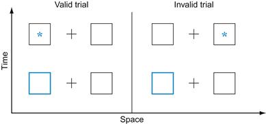
In the Posner paradigm, research participants are asked to fixate in the center of the screen and not to break fixation for the duration of the trial. Then, a location on the screen is cued in some way (usually by highlighting or flashing something). After the cue, a target appears in either the cued location or in another location. Research participants are instructed to press a key as soon as they see the target. Figure 7.1 provides a schematic illustration of the paradigm.
Posner (1984) found that if the cue is valid, reaction time was substantially lower than if it was invalid. He interpreted this in terms of an “attentional spotlight” that is focused on a certain region in space and permanently shifting at a finite and measurable speed.
7.3 Exercises
Most of the functions needed to write software that allows you to gather reaction time data were already introduced in Chapter 6, “Visual Search and Pop Out.” This time, we will introduce some functions that allow you to generalize the kinds of conditions in which such data are collected. To this end, we introduce another drawing function, rectangle, that will come in handy when creating your program in Section 7.4.
xlim([0 1]) %Set the range of values on the x-axis to (0 to 1)
ylim([0 1]) %Set the range of values on the y-axis to (0 to 1)
rectangle(‘Position’, [0.2 0.6 0.5 0.2]) %Create a rectangle at the x-position 0.2, %y-position 0.6 with an x-width of 0.5 and a y-height of 0.2
If you declare rectangle with a handle, you can change all properties of the rectangle. Try it. Rectangles have some interesting properties that can be changed.
Regarding data analysis, the most important function we can introduce at this point is the t-test. MATLAB uses ttest2 to test the hypothesis that there is a difference in the mean of two independent samples.
A = rand(100,1); %Create a matrix A with 100 random elements in one column
B = rand(100,1); %Create a matrix B with 100 random elements in one column
This means that the null hypothesis was kept because you failed to reject it. You failed to reject it because the observed difference in means (given the null hypothesis is true) had a probability of about 0.67, which is far too high to reject the null hypothesis. This is what you should expect if the random number generator works. Now try this test:
Now, the null hypothesis is rejected. As a matter of fact, the p-value is miniscule.
Note on seeding the random number generator: If you use the rand() function just as is, the SAME sequence of pseudorandom numbers will be generated each session. You can avoid this by seeding it first like this: rand(‘state’,number). It is important to note that the “random number generator” does no such thing. As a matter of fact, all numbers generated are perfectly deterministic, given the same seed number. We don’t want to go on a tangent why this has to be the case or how to avoid this by relying on a genuinely random (at least as far as we can tell) natural process (such as radioactive decay). As long as you pick a different number as a seed each time, you should be fine, for all common intents and purposes. Hence, it is popular to make the number after the state argument dependent on the cpu-clock. In old versions of MATLAB (e.g., 7.04), this could be done as follows:
Newer versions of MATLAB (e.g., 8.1 onwards) rely on a very different system. Namely, the notion of a random number stream that underlies rand, randn, and randi. This random number stream is implemented as randstream.
To seed the generator in new versions of MATLAB, things are more complicated but also more versatile.
First type
RandStream.list
to get a list of available pseudorandom number generation methods. Mersenne twister with Mersenne prime 2^19937-1 sounds appealing.
Note the value of “Seed”.
These changes are due to the fact that MATLAB is becoming increasingly object oriented. We are now handling Randstream “objects.” Expect to see more of this in the future. For the project in Section 7.4, it might be useful to know at least one other common data analysis function, namely ANOVA (analysis of variance). ANOVA generalizes the case of a two-sample t-test to many samples. For the purposes of this chapter, a one-way ANOVA will be sufficient:
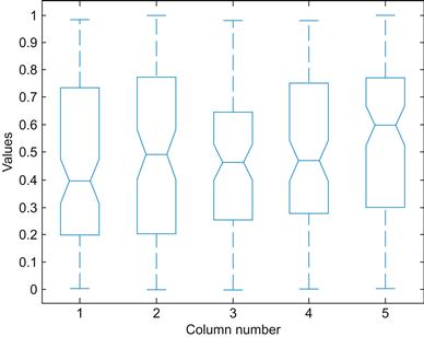
In this case, there were no significant differences, as revealed by Table 7.1 and Figure 7.2.
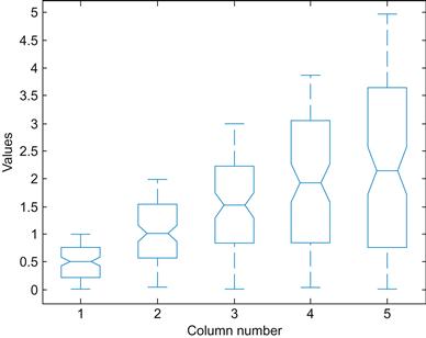
This time, there can be no doubt that there is a positive trend, as you can see in Table 7.2 and Figure 7.3.
The anova1 function assumes that different samples are stored in different columns and that different rows represent different observations in the same sample.
Note that anova1 assumes that there is an equal number of observations in each sample. For more generalized ANOVAs or unequal samples, see anova2 or anovan. Their syntax is very similar. This, however, should not be necessary for the following project.
7.4 Project
For this project, your task is to replicate a generalized version of the Posner paradigm. In essence, you will measure the speed of the “attentional spotlight” in the vertical versus horizontal directions. You need to create a program that allows you to gather data on reaction times in the Posner paradigm as described in the preceding sections. Most of the particular implementation is up to you (the nature of the cue, specific distances, etc.). However, be sure to implement the following:
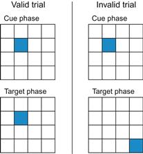
• Cue and target must appear in one of 16 possible positions. See, for example, Figure 7.4.
• Make sure you have an equal number of valid and invalid trials. [If the trial is valid, the target should appear in the position of the cue. If the trial is invalid, the target position should be picked randomly (minus 1, the position of the cue).]
• Choose two temporal delays between cue and target: 100 ms and 300 ms. Make the delay an experimental condition.
• Collect data from 80 trials per spatial location of the cue (so that you have 20 for each combination of conditions: Valid/invalid, delay1/delay2). This makes for a total of 1280 trials. But they will go very, very quickly in this paradigm.
• Make sure that the picking of condition (valid/invalid, delay1/delay2, spatial location of cue) is random.
• After collecting the data, answer the following questions:
1. Is there a difference in reaction times for valid versus invalid trials? (t-test)
2. Is there a difference in reaction times for different delays? (t-test)
3. Does the distance between target and cue matter? For this, use only invalid trials and plot reaction time as a function of
a. Total distance of cue and target
b. Horizontal distance of cue and target
c. Vertical distance of cue and target
4. Related to this: Is there a qualitative difference in the slope of these lines? Is the scanner faster in one dimension than the other?
5. What is the speed of the attentional scanner? How many (unit of your choice, could be inches) does it shift per millisecond?
• Implement the project in MATLAB and answer the preceding questions. Illustrate with figures where appropriate.
• *If you are adventurous: Use anova2 or anovan to look for interaction effects between type of trial (valid/invalid, delay and spatial location of cue).

Figure 7.4 Valid and invalid trials.
• Start writing one trial and make sure it works properly.
• Be aware that you effectively have an experimental design with three factors: Cue position (16 levels), trial type (2 levels), and temporal delay (2 levels). However, you can break it up into four factors: Horizontal cue position (4 levels), Vertical cue position (4 levels), trial type (2 levels), and temporal delay (2 levels), which will make it easier to assess the x- versus y-speed of the scanner.
• If you can’t produce a proper cue, try reviewing object handles (in figures).
• Write a big loop that goes through trials. Do this at the very end, if individual trials work.
• If you can’t do everything, focus on subgoals. Implement one function after the other. Start with two conditions. If you are not able to implement all eight conditions, try to get as far as you can.


