Neural Networks as Forest Fires
Stochastic Neurodynamics
The purpose of this chapter is to familiarize you with simulating a stochastic process. We will be modeling a large-scale network of firing neurons through the analogy of forest fires. In the process, you will become more adept at using convolutions and creating movies of neural population dynamics.
Keywords
stochastic process; quiescent neurons; active neurons; refractory neurons
35.1 Goals of This Chapter
The purpose of this chapter is to familiarize you with simulating a stochastic process. We will be modeling a large-scale network of firing neurons through the analogy of forest fires. In the process, you will become more adept at using convolutions and creating movies of neural population dynamics.
35.2 Background
The brain is made up of approximately 3×10¹⁰ neurons, each supporting up to 104 synaptic connections. Even after allowing for the specializations of neural circuitry that must exist to achieve coordinated activity, it is remarkable that such activity is not completely random. It seems reasonable, however, that large-scale neocortical activity has some random component, and thus its appropriate representation must be probabilistic. In creating a large-scale model of neuronal population dynamics that includes this probabilistic nature, we can use the analogy of a well-studied stochastic model of forest fires.
There exists a close correspondence between the dynamics and properties of large networks of spiking neurons and that of forest fires. In 1990, Bak, Chen, and Tang introduced the forest fire model, a probabilistic cellular automaton defined on a lattice. Each lattice site is occupied by either a green tree, a burning tree, or a burnt tree. The state of the system is updated by the following rules: (1) a burning tree becomes a burnt tree with probability 1; (2) a burnt tree grows into a green tree with probability p; (3) a green tree becomes a burning tree if at least one of its neighbors is burning, or if it is hit by lightning (with probability f.)
Just as a forest contains green, burning, or burnt trees, neural networks contain quiescent, active, or refractory neurons. When the membrane voltage V(t) of a neuron is above its resting potential (typically around −60 mV) and below the threshold potential (around −40 mV), the neuron is said to be in the quiescent state. It can be excited, just as a green tree can be ignited. When the membrane potential of the neuron exceeds the threshold, the neuron is active, and the membrane potential spikes to a large positive value for about a millisecond. Immediately afterwards, the neuron enters a refractory state, during which the membrane potential of the neuron is hyperpolarized. With a characteristic time constant determined by the membrane properties, the membrane potential returns to the resting potential and thus the neuron can return to the quiescent state (see Figure 35.1).
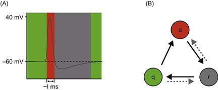
Figure 35.1 A. The membrane potential of a typical spiking neuron. When the membrane potential of the neuron is at or above its resting potential (dotted line) and below the threshold potential, the neuron is quiescent (green). After the neuron fires the action potential (red), the neuron enters a refractory state (black), during which the membrane potential of the neuron is less than the membrane potential. B. A neuron cycles through these states with time, given its membrane properties and input from connecting neurons (dotted lines indicate transitions that can occur with inhibitory input to the neuron).
Models of neuronal activity, both as standard forest fires as well as networks of integrate-and-fire neurons, are capable of displaying a variety of interesting behavior. These include long-range (power law) temporal correlations in the inter-spike interval histograms, stochastic resonance in the noise-driven appearance of spirals of neural activity, and traveling waves.
35.2.1 Neural Analysis
The key conjecture (introduced by Bak, Chen, and Tang (1990) and elaborated by Drossel and Schwabl (1992)) is that in the limit p → 0, f/p → 0 the dynamics of the forest fire become critical. In words, the first condition says that the state is critical as long as trees grow slowly, and the second condition guarantees that a lightning strike will destroy a large number of trees. A critical state of a driven dynamical system is one in which interactions between all its elements occur so that correlations develop at all length scales in the system. Such a state is marginally stable and can support large fluctuations. In the forest fire, this means that power law distributions of such quantities as the size of clusters of burning trees would develop as the forest dynamics tend to the critical limit.
In a neural network, 1/p is interpreted as the mean time it takes for a refractory neuron to recover sensitivity, and thus return to the quiescent state, while 1/f is the mean time between spontaneous activations of a neuron (produced, for example, by noise). An analysis in the context of stochastic neurodynamics was carried out by Buice and Cowan (2007). At first, we will consider a network of these simplified stochastic neurons that are connected in a very simple way, having either nearest neighbor or next-to-nearest neighbor excitatory connections.
35.3 Exercises
Our goal is to create a movie of the activity of an N×N array of neurons for T time frames, i.e., the spatiotemporal dynamics of the neurons will be modeled in an N×N×T matrix. Each pixel of the movie will either be green, red, or black to represent a neuron at that site and time in the quiescent, active, or refractory state, respectively. We begin by writing a function called ForestFireModel that will generate an avi file of the forest fire simulation that can be viewed outside of MATLAB® and that will take the following inputs: T, the number of iterations (time); p, the growth rate; f, the probability of spontaneous ignition; N, the lattice size; th, the threshold value. Furthermore, we will have the input BC to be able to set the boundary conditions for our simulation to be either free or periodic, and finally the input conn to be either 1 for nearest neighbor or 2 for next-to-nearest neighbor connectivity. This is a simple approach, without going so far as to design a GUI interface, to create a modeling environment in which you have numerous parameters that you may want to alter.
The downside to so many parameters, though, is that it could be inconvenient to populate them all of the time. Therefore it is useful to include a series of nargin statements at the top of our ForestFireModel function, providing a default set of parameters. Inside a function, nargin indicates how many input arguments have been given in the function call. We will use this to encode a good, working set of default parameters, and furthermore allow the function to be called without argument for convenience. Note the order in which these parameters are given.
function Forest=ForestFireModel(T,p,f,N,th,BC,conn)
% This function simulates a neural network as a forest fires
if nargin<7, conn=2; end %connectivity (1 nn, 2 nnn)
if nargin<6, BC=‘periodic’; end %Boundary Cond. (‘free’ or ‘periodic’)
if nargin<5, th=.1; end %threshold
if nargin<4, N=64; end %lattice size
if nargin<3, f=2e-4; end %prob of spontaneous ignition
if nargin<2, p=.1; end %growth rate
if nargin<1, T=100; end %number of iterations (time)
mov=avifile(‘Forest.avi’); %initialize the movie file that will be created
We are going to assign numerical values to the three possible states of the neuron:
Next, we create our initial “forest,” F, of neurons, an N×N matrix. The command rand(N) creates an N×N matrix of numbers uniformly distributed between 0 and 1, so rand(N)<0.4 creates a N×N matrix of 0s and 1s with a site being populated by 1 with a probability of 0.4. We can multiply this by 100 to make this a matrix of 0s and 100s—a forest with mainly quiescent trees (0s) and about 40% in the refractory state (100 s):
The connectivity matrix gives the weight of the connections of a given neuron to its neighbors. The center of the matrix is the location of the source neuron, and it will thus have a value of zero since we do not want to model self-stimulation. The weight of the connection to a cell is proportional to the distance from the source neuron. Here we use another MATLAB control structure, the switch/case statements:
%% ------------------------------
%% ------------------------------
%% Nearest neighbor interactions
%% Next-nearest neighbor interactions
W=[0 0 1 0 0; 0 sqrt(2) 2 sqrt(2) 0; ...
1 2 0 2 1; 0 sqrt(2) 2 sqrt(2) 0; 0 0 1 0 0];
We are now ready for the main loop of the simulation. This will use the built-in conv2 function for free boundary conditions, and the conv2_periodic.m function introduced in Chapter 16, “Convolution,” for the periodic boundary conditions.
%% -------------------------------
%% -------------------------------
Ac=(F==1); %id’s active fires in previous timestep
Qu=(F==0); %id’s quiescent trees in previous timestep
Rs=(F==100); %id’s refractive trees in previous timestep
CoA=conv2(double(Ac), W, ‘same’); %convolve fires w/ connectivity array
At this point we have defined three identifying matrices, Ac, Qu, and Rs, that are N×N matrices of 0s taking on the value of 1 only if that neuron is in the active, quiescent, or refractory state respectively. We have also created a matrix CoA that is the net input to all of the neurons. It was found by convolving the active neurons (those elements of the forest F with a value of 1 at time i ) with the connectivity matrix.
Now we create a temporary N×N matrix, Fr, which is all 0s and only takes on the value of 1 for those neurons who were in the quiescent state and whose input exceeded the threshold value. We also create another N×N temporary matrix, Frn, which is all 0s and only takes on the value of 1 with probability f if the neuron was in the quiescent state, but its input did not exceed threshold. The use of element-wise matrix multiplication of the identifying matrix Qu in the definition of these matrices ensures that only those sites that were in the quiescent state (having a value of 0 in the forest matrix F) take on a non-zero value. These two matrices identify those neurons in the forest that will transition from the quiescent state to the active state.
Fr=(CoA>th).*Qu; % id’s q trees whose input exceeded threshold
Frn=(Fr==0).*(rand(N)<f).*Qu; %with prob f selects trees from set q
%whose input does not exceed threshold
The forest matrix F is now updated by the transition rules:
F=100*Ac+100*(rand(N)>p).*Rs+Fr+Frn; %updates forest by rules
We can now redefine the identifying matrices:
The next few lines generate the movie of the simulation, and save it to an AVI file. The use of colormap(colorcube(12)) will cause a matrix element with a value of 7 to appear as a green pixel, an element with a value of 5 as red, and one with a value of 10 as black (see Figure 35.2):

Figure 35.2 A snapshot of the neural network simulated as a forest fire. Each pixel represents a single neuron, and it is colored green, red, or black to represent the neuron being in the quiescent, active, or refractory state, respectively.
The entire spatio-temporal dynamics of this network is saved in the N×N×T matrix, Forest, which can be loaded once the program has run using the command load Forest.
35.4 Projects
1. Of course, true neural networks are more complicated than forests. Neural dynamics are more complex than the simple ignition of a tree. In addition, there are two types of neurons: excitatory and inhibitory. About 25% of the neurons in the cortex of the brain are inhibitory; they act to prevent other neurons from activating. To some extent the first complexity doesn’t matter too much, but the existence of inhibition can radically alter neural network dynamics. There is also some evidence that the spatial extent of inhibition differs from that of excitation. This has profound consequences for the dynamics of neural activation.
Forest fire models have been developed by Drossel, Clar, and Schwabl (1994) in which trees have a certain immunity to fire, which acts like inhibition. Modify the forest fire model to incorporate inhibition. Create simulations for a network of randomly connected lattice sites in which proximal neighbor connections tend to be excitatory and more distal ones tend to be inhibitory (i.e., a Mexican hat distribution of excitatory and inhibitory interactions). You can take a peek at Chapter 16, “Convolution,” to help setup the connectivity matrix. What new patterns of activity are you able to produce? Can you find a parameter set that will create blobs or stripes?
2. The stochastic nature of the neuronal population can be introduced to the model in a number of places. Incorporate additional noise to the system by making the threshold follow Brownian motion within reflecting boundaries. Hint: you will need to introduce an N×N matrix that contains the threshold value for each of the neurons and is updated at each timestep. You will use the rand function to generate the amount by which the threshold value is increased or decreased at each step, and impose a minimum and maximum value that the threshold can be. If the random increment exceeds the boundary by an amount x, then the new value of the threshold is a distance x within the boundary.
3. For a more advanced project, modify the above simulations using noisy integrate-and-fire neurons to populate the forest. See what interesting population dynamics you can produce.