Neural Networks Part II
Supervised Learning
This chapter has two primary goals. The first goal is to be introduced to the concept of supervised learning and how it may relate to synaptic plasticity in the nervous system, particularly in the cerebellum. The second goal is to learn to implement single-layer and multi-layer neural network architectures using supervised learning rules to solve particular problems.
Keywords
supervised learning rule; perceptron; Widrow-Hoff learning rule; backpropagation; hyperplane
37.1 Goals of This Chapter
This chapter has two primary goals. The first goal is to be introduced to the concept of supervised learning and how it may relate to synaptic plasticity in the nervous system, particularly in the cerebellum. The second goal is to learn to implement single-layer (technically a two-layer network but the first layer is not always considered a true layer) and multi-layer neural network architectures using supervised learning rules to solve particular problems.
37.2 Background
37.2.1 Single-Layer Supervised Networks
Historically, perceptrons were the first neural networks to be developed, and they happened to employ a supervised learning rule. A supervised learning rule is one in which there is a teaching signal that provides the goal of the learning process. Inspired by the latest neuroscience research of the day, McCulloch and Pitts (1943) suggested that neurons might be able to implement logical operations. Specifically, they proposed a neuron with two binary inputs (0 or 1), a summing operation in the inputs, a threshold that can be met or not, and a binary output (0 or 1). In this way, logical operators like AND or OR can be implemented by such a neuron (by either firing or not firing if a threshold is met or not). See Table 37.1 from an example of implementing the logical AND operator with a threshold value of 2.
Later, Frank Rosenblatt (1958) used the McCulloch and Pitts Model in combination with theoretical developments by Hebb to create the first perceptron. It is a modified McCulloch and Pitts neuron, with an arbitrary number of weighted inputs. Moreover, the inputs can have any magnitude (not just binary), but the output of the neuron is 1 or 0 depending on whether the total weighted input exceeds the threshold or not. The weight can be different for each input. Setting the weights differently allows for more powerful computations.
Perceptrons are good at separating an input space into two parts (the output). Training a perceptron amounts to adjusting the weights and biases such that it rotates and shifts a line until the input space is properly partitioned. If the input space is higher than two-dimensions, the perceptron implements a hyperplane (with one dimension less than the input space) to partition it into two regions. If the network consists of multiple perceptrons, each can achieve one partition. The weights and biases are adjusted according to the perceptron learning rule:
1. If the output is correct, the weight vector associated with the neuron is not changed.
2. If the output is 0 and should have been 1, the input vector is added to the weight vector.
3. If the output is 1 and should have been 0, the input vector is subtracted from the weight vector.
It works by changing the weight vector to point more towards input vectors categorized as 1 and away from vectors categorized as 0.
Although a real neuron either fires an action potential or not (i.e., it generates a 1 or 0), the response of a neuron is often described by its firing rate (i.e., the number of spikes per unit time), resulting in a graded response (Adrian and Matthews, 1927). To model these responses, we use a different neural network model, called a linear network. The main difference between linear networks and perceptrons lies in the nature of the transfer function. Where the perceptron uses a step function to map inputs to (binary) outputs, a linear network has a linear transfer function. The learning rule for the linear network is called the Widrow-Hoff learning rule, and is essentially the same as that for the perceptron (Widrow and Hoff, 1960). This rule attempts to minimize the sum squared error between the target, T, and the output neurons’ (or, more properly, nodes’) activations, O, by going down the gradient of the error surface in the multi-dimensional weight space. The sum squared error is defined as the squared difference between target and output values summed over all the output neurons. The gradient is the derivative of the error with respect to each weight:
 (37.1)
 (37.2)
The output node’s activation is equal to the net input, net (i.e., the weighted sum of the activations of the input neurons, I), because the transfer function is linear:
 (37.3)
 (37.4)
 (37.5)
 (37.6)
where Δwij is the weight change between input node i and output node j, ε is the learning rate constant, Tj is the target on node j, Oj is the activation of output node j, and Ii is the activation of input node i. Equation 37.6 is the Widrow-Hoff learning rule. Since the error equation above is quadratic, this error function will have one global minimum (if it has any). Hence, we can be assured that the Widrow-Hoff rule will find this minimum by gradually descending into it from the starting point (given by the initial input weights). In other words, we are moving into the minimum of an error surface. MATLAB® has a visual demonstration of that: demolin1.
If the output node’s transfer function (i.e., activation function) is a differentiable, non-linear function, f(x), the Widrow-Hoff learning rule can be adjusted by changing Equation 37.4:
 (37.7)
 (37.8)
where  is the derivative of the non-linear transfer function evaluated at netj.
 (37.9)
 (37.10)
Let’s define the error as seen by output neuron Oj as δj:
 (37.11)
37.2.2 Multilayer Supervised Networks
Since perceptrons are vaunted for their ability to implement and solve logical functions, it came as quite a shock when Minsky and Papert (1959) showed that a single layer (technically a two-layer network but the first layer is sometimes not considered a true layer) perceptron could not solve a rather elementary logical function: XOR (exclusive or; see Figure 37.1). This finding also implies that all similar networks (linear networks, etc.) can only solve linearly separable problems. These events caused a sharp decrease in the interest in neural networks until its resurgence during the 1980s.
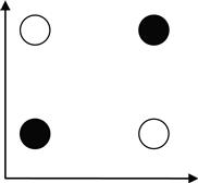
Figure 37.1 The XOR problem that a single layer network cannot solve. The XOR problem requires that the neuron respond (i.e., white circles) when only one (but not both) of the inputs is on. This is not solvable by a single-layer perceptron or linear network because it is not linearly separable.
The revived interest in neural networks occurred in part with the advent of multilayer, nonlinear networks with hidden units, and a learning rule used to train them called backpropagation, which is a generalized Widrow-Hoff rule. The power of these networks is that they can approximate any arbitrary nonlinear, differentiable function between the inputs and outputs.
The backpropagation (or backprop, for short) learning rule is a generalization of the Widrow-Hoff learning rule for multilayer, nonlinear networks that adjusts the weight between a pre- and postsynaptic node proportional to the product of the presynaptic activity and a measure of the error registered at the postsynaptic node. For nodes at the output layer, the error is straightforward. It is the difference between the target and the output node’s activity multiplied by the derivative of the non-linear activation function as in the single-layer, nonlinear case (see Equation 37.11). But what is the error for a hidden node? By using the chain rule for differentiation, backprop can define such an error as follows:
 (37.12)
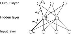
To derive this, let’s assume we have a network with four input nodes, three output nodes, and one hidden layer with two hidden nodes (Figure 37.2). Let’s define the input, hidden, and output layers as I, H, and O, and we will use subscripts m, l, and k to refer to particular nodes in each layer, respectively. Let’s also designate the weights feeding into the hidden nodes as wH, and the weights feeding into the output nodes as wO.
The partial derivative of the sum squared error with respect to a weight connecting an input node, i, to a hidden node, j, can be found by the following:
 (37.13)
 (37.14)
 (37.15)
 (37.16)
 (37.17)
 (37.18)
 (37.19)
 (37.20)
 (37.21)
 (37.22)
37.2.3 Supervised Learning in Neurobiology
Although there is no definitive evidence for neural plasticity that is guided by a “teaching” signal as supervised learning requires, there are some intriguing experimental findings which suggest the possibility that the physiology of the cerebellum may support a form of supervised plasticity. David Marr and James Albus independently proposed that the unique and regular anatomical architecture of the cerebellum could instantiate error-based plasticity that might underlie motor learning. In particular, they proposed that the climbing fibers acting on Purkinje cells from the inferior olive could provide an error signal to modify the synapses between the parallel fibers and the Purkinje cells. Experimental support for this theory first came from Ito and Kano (1982), who discovered that long-term depression could be induced at the synapse between the parallel fibers and the Purkinje cells. By electrically stimulating the parallel fibers and at the same time stimulating the climbing fibers (each of which forms strong synaptic contacts with a particular Purkinje cell), the parallel fiber synapse could be depressed. Because the Purkinje cells are inhibitory on the deep cerebellar nuclei, this synaptic depression would disinhibit the deep cerebellar nuclei.
A number of motor learning experiments have provided additional support for the idea that the cerebellum supports supervised learning via the climbing fibers. Sensory-motor adaptation experiments in which the gain between the movement and its sensory consequences are altered have shown transient increases in climbing fiber input (as measured by the complex spike rate) during learning (Ojakangas and Ebner, 1992, 1994). In addition, classical conditional experiments have suggested that the cerebellum plays a role in learning associations between unconditioned stimuli (US) and conditioned stimuli (CS) (Medina et al., 2000). For example, learning the association between an air puff (US) generating an eye-blink response and a tone (CS) is disrupted by reversible inactivation to parts of the cerebellum (Krupa, Thompson, and Thompson, 1993). Moreover, it has been shown that the tone enters the cerebellar cortex via the parallel fiber pathway, whereas the air puff (acting like a teacher) enters through the climbing fiber input. In fact, a mathematical formulation of classical conditioning proposed by Rescorla and Wagner (1972) quite closely resembles the Widrow-Hoff error correction learning rule using in supervised neural networks.
37.3 Exercises
37.3.1 Perceptrons
Start by creating a perceptron with two input nodes and one output node by creating a 1×2 weight matrix W (i.e., 1 output and 2 inputs) initialized to zero, a bias weight b initialized to zero, and a thresholding transfer function for the output unit:
If the net input to the output node is larger than 0, the output will be 1; otherwise it will be 0. A bias weight can be thought of as connecting an additional input node whose value is always 1 to the output node. The bias weight changes the point where this decision is made. For example, if the bias is −5, the net sum has to exceed 5 in order for the output to yield 1 (the bias of −5 is subtracted from the net sum; if it is less than 5, it will fall below 0).
Now set the weights from the two input nodes to 1 and −1, respectively. Set the bias weight to zero.
If the sum of the input multiplied by the weight meets or exceeds 0, the network should return 1; otherwise it should return 0. Test it by feeding it some inputs:
| inp1=[1; 0.5] | %Note: The first, positive weighted input larger than the second |
| inp2=[0.5; 1] | %Note: The second, negative weighted input is larger than the first |
Your output should be 1 for inp1 and 0 for inp2. The network classified these inputs correctly. You can now feed the network a large number of random numbers and see if they are classified correctly, like this:
| a=rand(2,10) | %Create 20 random numbers, arranged as 2 rows, 10 columns |
If the value in the first input row is larger than the value in the second input row (for a given column), the output value (for that column) should be 1; otherwise it should be 0.
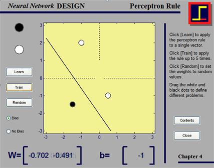
By adjusting the weights and the bias, it can be shown that any linearly separable problem (a problem space that can be separated by a line or more generally by a hyperplane) can be solved by a perceptron. To verify if this is the case, play around with the interactive perceptron, where you can arbitrarily set the decision boundary yourself. Type nnd4db (Figure 37.3). Try to separate the white and the black circles. They represent the inputs. The output is represented by the black line (creating two regions; presumably one region corresponding to an output of zero and another region corresponding to an output of one).
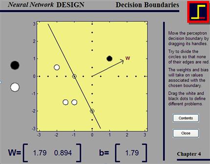
Figure 37.3 An interactive display of the decision boundary of a perceptron provided in the MATLAB Neural Network Toolbox. The display shows how a perceptron creates a linear decision boundary whose slope and intercept can be modified by adjusting the weight vector and bias.
What if you don’t know the weights or don’t want to find the weights? What if you only know the problem? Luckily, one of the strongest functions of neural networks is their ability to learn—to solve problems like this on their own. We will do this now. The first thing we need is a learning rule, a rule that tells us how to update the weights (and biases), given a certain existing relationship between input and output. The perceptron learning rule is an instance of supervised learning, giving the network pairs of inputs and desired (correct) outputs. The perceptron learning rule is essentially equivalent to the Widrow-Hoff learning rule:
To test this, set the weight matrix and bias weight back to zero. Use the random numbers you created as inputs and the correct answer as targets and train the network. You can try this dynamically, in an interactive demo, by typing nnd4pr (see Figure 37.4).
37.3.2 Linear Networks
Now you will create a linear network with two input nodes and one output node. The only difference between a linear network and a perceptron is the transfer function of the output node. The output node’s activation is simply equal to the net input:
Set the weights to 3 and 4 and bias to 0, and feed the network the following input:
The same can be done by typing:
In other words, this neural network implements an inner product (dot product).
Of course, we want a more useful neural net than just one that can take the dot product; we can take the dot product without neural nets. A classical function of linear neural networks is the automatic classification of input objects into different categories. In order to achieve that, we need to train the network. To do this, we will use the Widrow-Hoff learning rule again. However, this time we will feed the inputs and targets multiple times (i.e., through multiple epochs), each time incrementing the weights by a small amount scaled by a learning rate parameter ε:
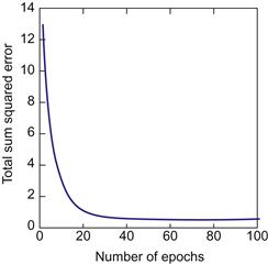
To assess the quality of learning, we will measure the total sum squared error between the output of the network and the target summed over all output units k and all training samples p after each epoch of learning:

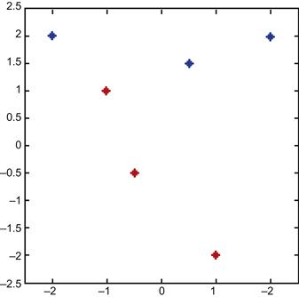
Why not give it a try? Say we have six two-dimensional inputs from two sets: set1 and set2.
Plot them to see what is going on:
>> plot(set1(:,1),set1(:,2),’*’) %Plotting the first set
>> plot(set2(:,1),set2(:,2),’*’, ’color’, ’r’)
Looking at the graph, you can see what is going on (Figure 37.5). We also see that the problem is, in principle, solvable; we can draw a line that separates the blue and the red stars. Now create a network that will find this solution, starting at 0 weights and 0 bias.
Next, assign the corresponding targets. We arbitrarily assign 1 to the blue set and 0 to the red set:
Finally, you have to decide on the learning rate, ε, and the number of times you run through the entire training data set (i.e., the number of epochs). Set the learning rate to 0.01 and the number of epochs to 100 (Figure 37.6).
Challenge the trained network with some new input, and see if it correctly classifies it. Pick something in the middle of the red range, like [−1, 0]. You should get 0.20 as an output. Of course, this should be 0. But this might be the best we can do, given the sparse input.
A linear classifier allows one to roughly categorize and classify inputs if they are linearly separable. Adjusting the weights and biases amounts to creating a linear transfer function that separates the desired outputs maximally and optimally. Of course, there is only so much that a linear function can do, but it’s not too bad.
Note that there is some initial classification even without training (Figure 37.7, left side). But it is not very good, and the absolute output values are all over the place. The final classification by the linear network is pretty good (Figure 37.7, right side). Values cluster around 1 and 0, although there is quite a bit of variance. The linear network couldn’t separate the clusters any better than this, given the variance in the input and the amount of training. You should always check your network by visualizing the outputs of trained and untrained networks with simple plots like this.
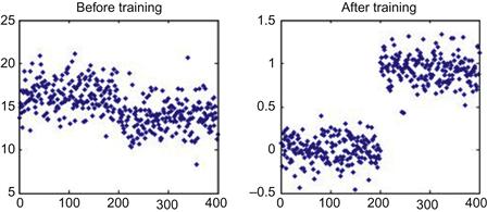
Figure 37.7 The problem of categorizing “good” and “bad” Greebles using a supervised linear network (see Chapter 36). Left: Classification when all the weights are set to 1 (before training). Right: Classification after application of the supervised learning rule (after training).
37.3.3 Backpropagation
Most of the principles of backpropagation are the same as in the other networks, but we now have to specify the number of layers, the number of input nodes, hidden nodes per hidden layer, and output nodes, and nonlinear transfer functions of the hidden and output nodes. For example, create a three-layer, feedforward network (i.e., one input layer, one hidden layer, and one output layer) with a sigmoidal transfer function:

The last line of code defines a function handle called transfer_fn to a sigmoid function whose output ranges from 0 to 1. The steepness of the sigmoid is specified by alpha.
The backprop learning rule applied to the weights feeding the output nodes is identical to the non-linear Widrow-Hoff learning rule (see Equation 37.10). However, for the weights feeding the hidden units, the rule is specified in Equation 37.21.
37.3.4 Sound Manipulation in MATLAB
As you saw in earlier chapters, MATLAB is not only useful for analyzing data; it is also possible to use it for experimental control and data gathering. Here, you will see that MATLAB can be used to design the stimulus material itself. Before you start, check the volume control to make sure that the loudspeaker of your PC is not muted and that the volume is turned up. There are many MATLAB functions dealing with auditory information; as a matter of fact, there is a whole toolbox devoted to it. Here, we will only handle sound in very fundamental ways.
The first thing you might want to do is to create your sound stimuli. To do so, try this:
Did you hear anything? What about this:
You know that your code created sine functions of increasing frequency. What you are listening to is the auditory representation of these sine functions, pure sine waves. Of course, most acoustic signals are not that pure. Try this to listen to the sound of randomness, white noise:
The sound function interprets the entries in an array (here, the array “x”) as amplitude values, and plays them as sound via your speakers. That means you can manipulate psychological qualities of the sound by MATLAB operations. You already saw how to manipulate pitch (by manipulating the frequency). You can manipulate volume by changing the magnitude of the values in the array. Sound expects values in the range 1 to −1. So how does this sound?
This should sound much less violent.
Of course, you can manipulate the sound in any way you want; for example, you can mix two signals:
This should sound like the sine wave from before, plus noise.
In short, what you hear should sound more complex, and rightfully so. It can be shown that any arbitrarily complex sound pattern (or any signal, really) can be constructed by appropriately adding sine waves. We will use this property later. Speaking of complex sounds, most practical applications will require you to deal with sounds that are much more complex than pure sine waves. So let’s look at one. Luckily, MATLAB comes with a complex sound bite:
You might be confused by the second parameter, Fs. It is the sampling rate at which the signal was sampled. It specifies how many amplitude values are played per second. If your array has 10,000 elements and the sampling rate is 10,000, it takes one second to play it as sound.
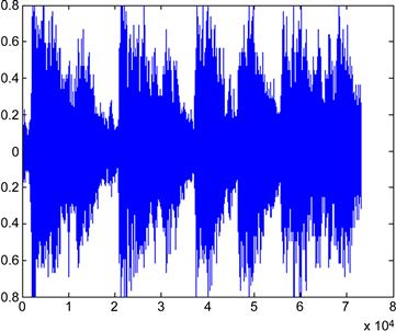
Why don’t we take a look at the structure of the amplitude values in the y matrix? This could help you understand how sound works.
This will do the trick, and it should look something like Figure 37.8.
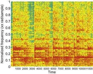
If you already listened to it, this will probably not surprise you. As a matter of fact, this information about sound amplitudes is not very powerful in itself. It is much better and more useful to look at the spectral power of a signal over time. To do this, we will use a function called spectrogram. It comes with the MATLAB Signal Processing Toolbox.
We won’t go into how exactly this function works. It is rather complex, and we could spend a whole chapter on it alone. In principle, let’s say that it decomposes the signal into sine waves and plots the power (how much of each frequency is in the signal) over time. A spectrogram of the Handel sounds looks like Figure 37.9.
The parameter, 256, breaks up the data into 256 segments and applies a Hamming window to each segment. ’yaxis’ specifies that the frequency axis should be plotted on the y-axis. Of course, you probably will want to import your own sounds into MATLAB. That can be done using the wavread function. Load the appropriate files that we have created, then type:
In this section, you saw how MATLAB lets you create, manipulate, and analyze acoustic stimuli. You can use it to design sound stimuli that are precisely timed and have very specific properties. Obviously, this is extremely useful for acoustic experiments.
37.4 Project
The project is to create a network that correctly classifies the gender of two target speech bites. In order to do this, train the network with a total of six speech bites of both genders. Load these files (called Train_Kira1 to 3 and Train_Pascal1 to 3). Of course, the two speakers differ in all kinds of ways other than just gender (age, race, English as a first/second language, idiosyncratic speech characteristics, lifestyle, etc.). If one were to face this problem in real life, one would have to train the network with a large number of speakers from both genders so that the network can extract gender information abstract from all these irrelevant dimensions. But for our purposes, this will be fine. Specifically, you should do the following:
Create a network that reliably distinguishes the gender of the two target speech bites. Provide some evidence that this is the case and submit the source code.
• You should implement a network using the backpropagation learning rule.
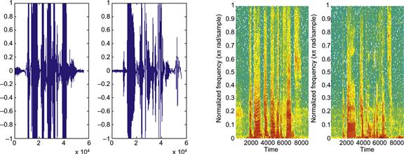
• Take the spectrogram of the sound files. Use those as the inputs to your neural network. See Figure 37.10 for the amplitude and spectrogram of the sentence “The dog jumped over the fence.” The left subplot is a female speaker, and the right subplot is a male speaker.
• a=spectrogram(b, 256) will return an array of complex numbers in a. They have an imaginary and a real part. For our purposes, the real part will do. For this, type
c=real(a). c will now contain the real part of the complex numbers in a.
• This project is deliberately under-constrained. Basically, you can try whatever you want to solve the problem. As a matter of fact, we encourage this, since it will help you understand neural networks that much better. Don’t be frustrated, and don’t panic if you can’t figure it out right away.
• If you take a spectrogram of the speech patterns with which you are supposed to train the network, it will return 129 rows and multiple columns. A neural network that takes the entire information from this matrix has to have 129 inputs.
• This is obviously rather excessive. If you closely observe the spectrogram (see Figure 37.10, right), you might be able to get away with less. The rows tessellate the frequency spectrum (y axis). Power in a particular frequency band is at a particular row. Power in a particular frequency band at a particular time is in a particular combination of row and column.
• The point is that the left spectrogram has much more power in the upper frequencies than the one on the right. If you properly combine frequency bands (or sample them), you might be able to get away with a neural network that has only five or ten inputs.
• The same applies for time. Your spectrogram will have several thousand columns. This kind of resolution is not necessary to get the job done. Try combining (averaging) the values in 100 or so columns into one. Then feed that to the neural network for training.
• Try having a large number of hidden units (definitely more than 1).
• You will be using a supervised learning rule. The target is defined by which file the data came from (Pascal or Kira). Create an artificial index, assigning 1 and 0 or 1 and 2 to each.
• Always remember what the rows and columns of the variables you are using represent. Be aware of transformations in dimensions.

