8

Fluid-Flow Measurements

8-1.  INTRODUCTION

Fluid flow touches every aspect of engineering, from industrial processing to research. Flow measurements and control are described in books and symposiums [1]. Surveys of the subject are published periodically in journals [2]. General-purpose flowmeters are often updated for high-tech applications [3].

Fluid flow measurement is a diverse field of study, which includes liquid and gas, compressible and incompressible, subsonic and supersonic, laminar and turbulent flow, steady state and pulsating, average flow and flow field, volumetric and mass flow, two-phase medium and slurry, closed and open channel. Flow measurements are influenced by a host of parameters, such as viscosity, temperature, pressure, and specific heat. Moreover, there are important variations within a class of flowmeters. In view of the diversity, this brief study cannot be comprehensive.

In this chapter we present a perspective of flowmeters by classifying flow measurements as “direct” and “indirect.” The study is mostly for flow in closed channels. It is important to note that the direct method to be described is not the direct comparison or null-balance method presented in Chapter 3.

Flow is a transport phenomenon. This allows a “direct” measurement. Flow can also be measured by its effect. This is loosely called an “indirect” measurement. In other words, any variable in a flow-related equation can be utilized for a flow measurement. This approach is used in Secs. 7-6 and 7-8 for the discussion of force and pressure transducers. It is hoped that a perspective can be gained by illustrating the principles and physical laws employed, pointing out variations of the same principle, showing sufficient examples, and discussing some applications. For convenience, conversions of commonly used units to SI for flow measurements are shown in Table 8-1.

TABLE 8-1 Conversions to SI Units

To convert from:	To:a	Multiply by:
barrel (for petroleum)	m3	1.589 873 E-1
centipoise	Pa·s	1.000 000 E-3
centistoke	m2/s	1.000 000 E-6
foot	m	3.048 000 E-1
foot-pound-force	J	1.355 818 E+0
gallon (U.S. liquid)	m3	3.785 412 E-3
pound-force	N	4.448 222 E+0
pound-force/in2	Pa	6.894 757 E+3
pound-mass	kg	4.535 924 E-1

^am, meter; N, newton, Pa, pascal, J, joule, kg, kilogram; 1N = 1 kg · m/s²,1 Pa = 1 N/m² = 1 kg/(m · s²).

8-2.  LAMINAR AND TURBULENT FLOW

Reynolds number, viscosity, laminar flow, and turbulent flow of incompressible fluids are examined briefly in this section. Turbulent flow occurs in mostflowmeters.

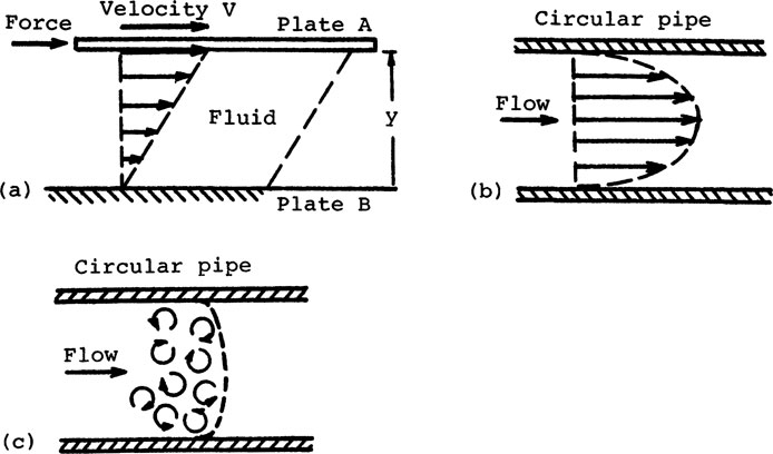
Viscous force of a fluid is an internal frictional force. Let plate A shown in Fig. 8-1a move in a fluid with a velocity V parallel to a stationary plate B. Thin layers of fluid adhere to the plates. The flow profile is as shown in the figure. Absolute (dynamic) viscosity of the fluid is defined as

$\text{absolute viscosity,μ=}\frac{\text{shear stress}}{\text{rate of shear strain}}$

(8-1)

$\text{μ=}\frac{\text{force}/\text{area}}{\left(\text{velocity }V\right)/\left(\text{distance }y\right)}$

(8-2)

An absolute (or dynamic) viscosity of 1 poise is 0.1 Pa · s or 0.1 kg/(m · s). The centipoise, or 0.01 poise, is a common unit. Its conversion to SI unitsis shown in Table 8-1. Kinematic viscosity is absolute viscosity divided by density. The common unit is the centistoke, expressed in units of m²/s. The stress/strain ratio in Eq. 8-1 resembles a shear modulus. A fluid in static equilibrium cannot sustain a shear stress as in a solid. Viscosity is due to the rate of shear strain between laminas of a fluid. The velocity gradient dV/dy is assumed constant. Viscosity is nonlinear for some fluids, such as greases.

The flow characteristics of fluids are described by the Reynolds number N_R, which is

FIGURE 8-1 Laminar and turbulent flow in fluids. (a) Flow between parallel plates.

$\text{Reynolds number,}{N}_R=\frac{\text{inertia force}}{\text{viscous force}}$

(8-3)

It can be shown from dimensional analysis that inertia force is proportional to D²ρV² and viscous force to μVD, whereρ is the fluid density in kg/m³, V its velocity in m/s, D a characteristic dimension in meters (such as a pipe diameter), and μ the absolute viscosity in Pa·s. Thus N_R in SI units reduces to

$N_R=\frac{\text{ρ}VD}{\text{μ}}$

(8-4)

In English units, ρ is in lb_m/ft³, V in ft/sec, D in feet, and μ in lb_f·sec/ft². Since N_R is nondimensional, it must be written as N_R = ρVD/μg_c, where g_c = 32.17 lb_m·ft/lb_f·sec² is a dimensional constant. Note that g_c in SI units is 1 kg.m/N·s² and it is not necessary in Eq. 8-4.

Laminar flow in a pipe, shown in Fig. 8-1b, occurs at low N_R when the viscous force dominates (see Eq. 8-3). Conditions for laminar flow are low density, low velocity, small diameter, and high viscosity, as shown in Eq. 8-4. The opposite is true for turbulent flow, as shown in Fig. 8-1c. This occurs at high N_R when the inertia force dominates. From experimental studies, the N_R for a transition from laminar to turbulent flow is from 2000 to 3000. The flow for this range is unstable.

Since N_R is based on dimensional analysis, relations obtained for one fluid are applicable for another fluid. For example, the drag coefficient of a circular disk versus Reynolds number is universally applicable for all fluids. This is the basis for target flowmeters described in a later section.

Flowmeters for viscous (laminar) flow at low N_R are governed by the Hagen-Poiseuille law.

$Q=\frac{\text{π}{r}^4}{8\text{μ}L}\text{Δ}P$

(8-5)

where Q is the volumetric flow rate, r the tube radius, μ the absolute viscosity, L the tube length, and ΔP the pressure drop. Flowmeters for turbulent flow at high N_R are governed by the square-root law. It can be shown from Bernoulli equation (Eq. 7-48) that the volumetric flow rate Q is proportional to the square root of the differential pressure ΔP across the flowmeter:

$Q=C\sqrt{\text{Δ}P}$

(8-6)

where C is a constant. The equation is derived in Sec. 8-5. Many types of flowmeters are governed by the square-root law and characteristics of square-root-law flowmeters are examined in Sec. 8-5B.

8-3.  DIRECT FLOW MEASUREMENTS

Flow is a transport phenomenon. Hence it can be measured directly. These methods can be classified as (1) weighing or volumetric, (2) positive displacement, (3) flow visualization, and (4) tracer technique. A tracer is a carrier in the sense that it moves with the flow and carries the flow information.

A.  Weighing and Volumetric Methods

Flow measurement by a weighing or volumetric method removes the fluid from a system and integrates the flow rate over a specific period. The procedure is basic and conceptually simple, but it is not always convenient for field applications.

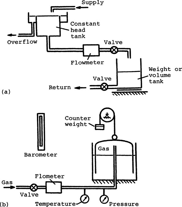
With proper precautions and procedures, this is the most accurate method. It relates a flow rate to the fundamental units of mass, length, and time. The uncertainty in measurement is of the order of 1 part in 10³[4]. It is often used for the steady-state calibration of other flowmeters, as shown schematically in Fig. 8-2.

FIGURE 8-2 Calibration of flowmeters. (a) Calibration of liquid flowmeter. (b) Calibration of gas flowmeter. (From Ref. 5.)

B. Positive-Displacement Meters

A positive-displacement meter measures volumetric flow rate by dividing the flow into segments. If each segment has a precise volume, the number of segments counted is the total volume.

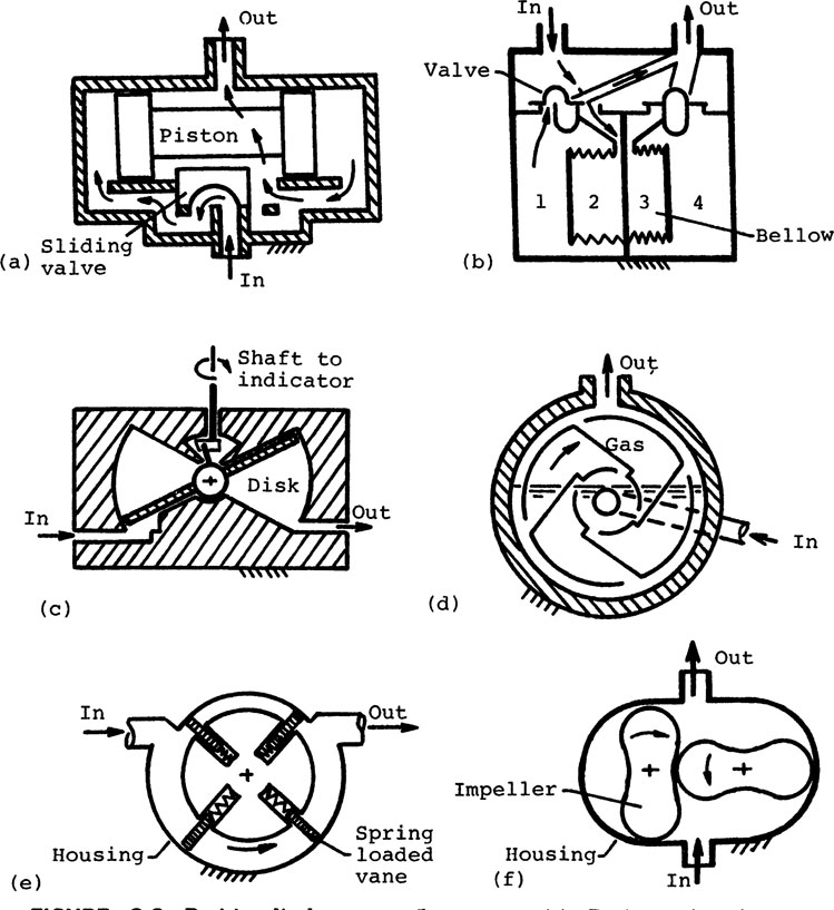
These flowmeters can be classified as reciprocating or rotary. Various constructions are used for both types. The reciprocating piston flowmeter in Fig. 8-3a is for liquids. The bellow type in Fig. 8-3b is for gases. As shownin the figure, chamber 1 is emptying to the outlet, chamber 2 is filling fromthe inlet, chamber 3 is empty, and chamber 4 is just filled. The gas flow is less pulsating by employing four chambers.

FIGURE 8-3 Positive-displacement flowmeters. (a) Reciprocating-piston meter. (b) Bellow-type meter (from Ref. 6). (c) Nutating-disk meter. (d) Sealed-drum meter. (e) Rotating-vane meter. (f) Lobed-impeller meter.

Four rotary flowmeters are shown in Fig. 8-3c to f. The nutating-disk meter is similar to a household water meter. The wet-type sealed-drum gas meter is superseded by the dry-type, because the liquid seal is subjected to freezing and evaporation. The rotary-vane meter is generally for liquids. The lobed-impeller meter is for liquid or gas. Many variations of the lobes are in use, including helical lobes, oval-shaped gears, and meters with more than two rotating parts.

The positive-displacement flowmeters above are essentially fluid motors. The pressure drop across the meter, typically 10 to 40 psi, is due to restrictions in the meter and friction of the moving parts. The accuracy is of the order of 1%, depending on the viscosity and the type of fluid. The performance of the meter will deteriorate with time because of wear and increasing leakages.

Positive-displacement meters are favored for start/stop short runs, medium-and high-viscosity fluids, and certain contaminated products. Their applications include tank truck metering, blending operations, refinery processing, and processes in crude oil production [7].

C.  Flow Visualization

Flow visualization [8] utilizes the flow stream itself for a qualitative and/or quantitative measurement of a flow field. Generally, the flow-related change in a property of fluid in the flow stream is examined, and the flow can be observed with minimum disturbance. A tracer is sometimes introduced in the fluid, assuming that the tracer follows the flow pattern and the flow pattern is least disturbed. The method is useful for research but rather inconvenient for most industrial applications.

Flow visualization for flow at low velocities [9] is well established. Smoke is commonly used as a tracer in airstreams. The smoke is generated by permitting air saturated with hydrochloric acid to come into contact with fumes of ammonia. Color dyes can be introduced in a fluid stream. Quantitative data for a three-dimensional flow can be obtained by using small particles of polystyrene suspended in the air and a stroboscopic light [10]. Oil can be injected in water with an atomizer. The oil droplets in suspension can be illuminated sharply by means of a thin sheet of light. Small pieces of aluminum and mica are suitable aids for flow visualization.

Schlieren, shadowgraph, and interferometry can be used for supersonic flows[11]. Schlieren and shadowgraph methods make use of the reflection of light due to variations in density in a compressible flow, similar to the passage of light through a glass prism. Interferometry makes use of changes in the speed of light passing through regions of varying density in a compressible flow. Quantitative data can be obtained from fringes (see Fig. 7-3) due to the interference between the affected and unaffected light beams.

D.  Carrier Systems

The term carrier systems is coined to describe a large class of flowmeters suitable for industrial applications. It is a tracer technique. A carrier moves with the flow and carries the flow information. Similar to flow visualization, the method is direct because the fluid itself is used to convey the flow information. Typical examples are described in this section.

The term carrier or tracer is used in the broad sense. It may be injected externally into a flow stream, such as radioisotopes, or be inherent in the fluid, such as air bubbles. The method can be used to obtain an average steady-state flow velocity or to probe the local velocity in a fluid. For an average velocity measurement, the tracer may not reveal the true profile of the flow, and the accuracy of measurement is influenced by this uncertainty.

1.  Electrolytic Tracers [12]

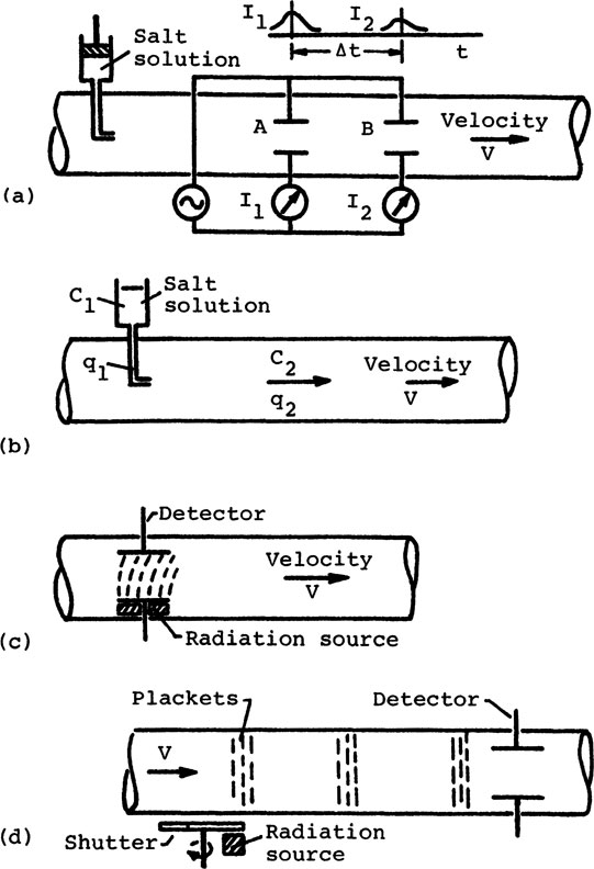
A transit time method is shown in Fig. 8-4a. A shot of salt solution is injected into the water in a pipe. The subsequent cloud of electrolyte in the water has higher conductivity than the water. Electric currents I₁ and I₂ are detected as the cloud of electrolyte passes the electrodes at A and B, separated by a distance L. The time difference or the transit time between I₁ and I₂ is Δt. The average velocity is V = L/Δt. The volumetric flow rate is the product of V and the cross-sectional area of the pipe.

The method is used for intermittent measurement of constant flow rates in large pipes. The accuracy is from 1 to 6%. The actual flow rate tends to be larger than that indicated, but the accuracy improves with higher Reynolds number because of greater turbulence. Error due to uncertainties in At can be minimized by using the At between the center of gravity of the current-time areas, as shown in the figure.

Alternatively, the volumetric flow rate can be determined by the dilution method, shown in Fig. 8-4b. A salt solution of concentration C₁ is introduced into the water at a steady and known flow rate q₁. The flow rate of the water q₂ is unknown. The concentration after mixing is C₂. Thus q₂ = q₁(C₁/C₂). The accuracy of the method is from 0.03 to 0.06% [13].

2.  Radioisotope Tracers

Radioisotope tracers can be substituted for the salt solution for both the transit time and the dilution method described above. Moreover, in using the dilution method, a sample of the fluid, either liquid or gas, can be withdrawn down stream from the point of injection. A more precise reading can be obtained by counting the radiation off-line. The number of counts is inversely proportional to the average velocity of the flow. Krypton 85 and argon 41 have been used to measure gas flow rates [14],

FIGURE 8-4 Tracer methods for flow measurement. (a) Transit-time method. (b) Dilution method. (c) Deflection method. (d) Signal modulation.

The deflection method probes the flow in a gas stream at only one location, as shown in Fig. 8-4c. The radiation is from an alpha or a beta soruce. For zero flow, almost all the ions are collected at the detector from the continuous ionization. As the gas velocity increases, some ions are swept out by the flow before they are collected. The ions collected can be correlated with the gas velocity.

A signal modulation method, shown in Fig. 8-4d, consists of a radiation source, a shutter, and a detector. The shutter is a rotating slotted disk. It modulates the constant radiation source to produce a sequence of ion plackets in the flow stream. The technique eliminates the dependence on gas composition, temperature, pressure, viscosity, humidity, and the inherent instability of ion-current-detecting electronics [15].

3.  Sonic Flowmeters [16]

Sonic or ultrasound flowmeters are applicable for pipe lines and open channels. The accuracy depends on the installation, operating conditions, and measuring technique. Accuracy of 0.02% is attainable [17]. A sales catalog [18] can be used as a guide, but the ultimate test of accuracy is by means of a field calibration [19].

The sonic method is generally considered a transit-time measurement. The flowmeter consists of a transmitter and a receiver; piezoelectric crystals are commonly used for both. The frequency of sonic signals is from 600 kHz to 10 MHz. Three basic techniques or their combinations are used: (1) transit time, (2) beam deflection, and (3) Doppler effect. Doppler effect describes the apparent frequency shift when a sonic wave is superposed on a flowing medium. An example is the increase in pitch of a train whistle as the train approaches an observer, followed by a decrease in pitch as the train passes and moves away from the observer.

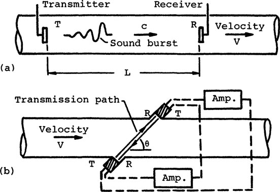
a. Transit-time method. Several methods using the transit-time technique and Doppler effect are described in this section. A sound burst or a train of sonic pulses is injected into a flowing fluid by means of a transmitter T and detected by a receiver R, as shown in Fig. 8-5a. When the sonic wave is injected downstream, the actual velocity of the wave is (c + V), where c (= 5000 ft/sec for water) is the sonic velocity in the fluid at rest and V the flow velocity. For a distance L between T and R, the transit time is t₁ = L/(c – V). Similarly, the transit time is t₂ = L/(c – V) when the sonic wave is injected upstream. Assuming that c ≫ V, the time difference Δt is

FIGURE 8-5 Ultrasound transit-time methods. (a) Basic transit-time method. (b) Nonintrusive transit-time method.

$\begin{array}{lll}\Delta t\hfill & =\hfill & t_2-t_1=\frac{L}{c-V}-\frac{L}{c+V}=\frac{2LV}{c^2-V^2}\hfill \\ \hfill & \simeq \hfill & \frac{2LV}{c^2}\hfill \end{array}$

(8-7)

An application of this method using four transducers is shown in Fig. 8-5b. If a transducer is used for both transmitting and receiving by time sharing, only two instead of the four transducers are required. The transducers are nonintrusive, and they can be clamped on the outside wall of a pipe. Note that this is a variation of the two-point transit-time method (see Fig. 8-4a) with the sonic wave superposed on the flow.

This technique is used successfully for large-diameter pipes, but the Δt is quite small and the uncertainty in its measurement can be large. For example, if c = 5 × 10³ ft/sec, L = 6 in., and V = 1 ft/sec, the Δt from Eq. 8-7 is 40 × 10⁻⁹ sec. When the leading edge of the pulse is used to indicate the pulse arrival time, error due to the overall pulse length or envelope shape has little effect on the measurement. The sonic velocity c, however, is not constant and is a function of fluid composition, temperature, and density.

The phase difference Δϕ between the upstream and downstream signals can be used to measure the flow velocity V instead of Δt. When a sinusoidal signal of frequency f is used, the Δϕ from Eq. 8-7 is

$\Delta \varphi =2\text{π}f\Delta t=\frac{4\text{π}fLV}{c^2-V^2}$

(8-8)

This technique is subject to the same limitation as the transit time method, because the associated electronics use Δt for determining the phase angle.

A frequency difference method using two resonant circuits is widely used. A resonant circuit is created by using the pulses received to trigger the transmitting pulses in a feedback loop. The feedback paths for the two resonant circuits are shown as dashed lines in Fig. 8-5b. The resonant frequencies f₁ and f₂ and the frequency difference Δf are

$\begin{array}{lll}{f}_1=\frac{1}{t_1}=\frac{c+V}{L}\hfill & \text{and}\hfill & f_2=\frac{1}{t_2}=\frac{c-V}{L}\hfill \end{array}$

(8-9)

$\Delta f=\frac{1}{t_1}-\frac{1}{t_2}=\frac{2V}{L}$

(8-10)

The method is independent of the sonic velocity c, but Δf tends to be small.

For the methods described above, if D is the internal diameter of the pipe and θ the angle as shown in Fig. 8-5b, then Δt, Δϕ, and Δf in Eqs. 8-7, 10 become

$\Delta t=\frac{2DV/\tan \theta }{c^2-{\left(V\cos \theta \right)}^2}$

(8-11)

$\Delta \varphi =\frac{2\text{π}f/\tan \theta }{c^2-{\left(V\cos \theta \right)}^2}$

(8-12)

$\Delta f=\frac{V\sin 2\theta }{D}$

(8-13)

b. Deflection method. In principle, the deflection method using ultrasound is similar to that using radiation shown in Fig. 8-4c. The transmitter and receiver are perpendicular to the pipe axis and separated by adistance L. The fluid flow with velocity V causes the sonic emission E to deflect by an amount X.

$X=\frac{V}{c}LE$

(8-14)

where c is the sonic velocity in the fluid at rest. Again, c is not constant. An additional uncertainty in the measurement is the strength of the emission E.

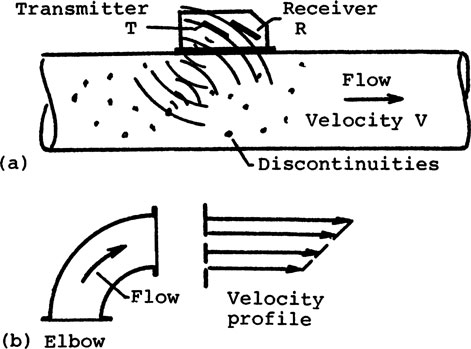
c. Doppler shift method [20]. A clamp-on Doppler flowmeter with a transmitter T and a receiver R as a single unit is shown in Fig. 8-6, although T and R may be separate units placed around the circumference of a pipe. T injects a continuous ultrasound beam at a frequency f_T (about 600 kHz) into the liquid. The beam is scattered by solid particles, bubbles, or any discontinuity in the liquid and is reflected back to R at a frequency f_R. The Doppler shift due to the velocity V of the liquid is the difference Δf = f_T–f_R.

FIGURE 8-6 Effect of velocity profile on Doppler meter. (a) Doppler flowmeter. (b) Flow profile due to elbow.

$\Delta f=f_T-f_R=\frac{2f_{T}V\cos \theta }{c}$

(8-15)

where c is the sonic velocity in the liquid at rest, 9 the angle as shown in Fig. 8-5b, and c ≫ V.

The Doppler effect measures the point value at a discontinuity. Since discontinuities are dispersed in a liquid, the receiver detects multiple frequencies. Some averaging scheme is used to obtain an average velocity for the volumetric flow rate. Hence the flowmeter is sensitive to the velocity profile across a flow section, as illustrated in Fig. 8-6b. In other words, changing the location of a flowmeter could invalidate its calibration.

In addition to the transducer location, other uncertainties to be considered are concentration of sonic discontinuities, size of suspended particles, depth of penetration of the ultrasonic beam, and air pockets in a pipe [21]. Note that a Doppler flowmeter depends on discontinuities in a liquid for its operation, while a transit-time meter must work with clean liquids to minimize signal attenuation and dispersion.

Doppler flowmeters are commonly used to measure industrial waste and mineral slurries. They are used successfully in such industries as papermaking, pharmaceuticals, and sewage disposal.

4.  Laser Velocimeter [22]

A laser velocimeter utilizes a frequency shift due to the scattering of a laser beam to measure local fluid velocities. It is suitable for measurements in liquids and gases. Both the Doppler flowmeter and the laser velocimeter employ the same principle; one is sonic and the other optical. Their operations can be compared by the similarity in properties of sound and light waves [23]. The laser velocimeter, however, is more complex.

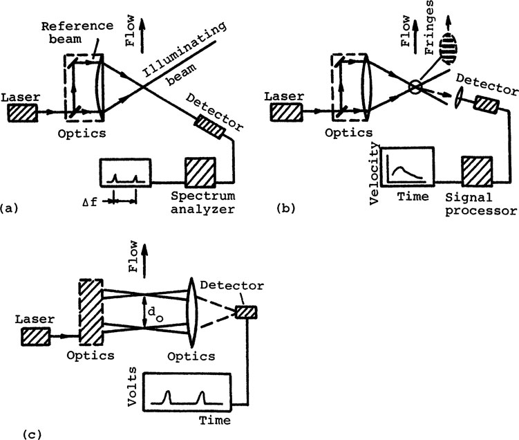
Many optical configurations have been proposed [24], and three commonly used ones are described briefly below [25]. The one shown schematically in Fig. 8-7a is based on the Doppler frequency shift from light scattered by particles moving with the flow. The frequency shift is small, but the light can be mixed (heterodyned) with the unshifted light from the laser. The mixing produces a beat frequency, equal to the frequency difference Δf of the Doppler shift. The flow velocity is proportional to Δf, as shown in the figure.

The dual-scatter system shown in Fig. 8-7b is called the differential mode or the fringe method. Due to scattering, a set of fringes (see also Fig. 7-3d) is formed from the optical interference of the two beams intersecting at the probed volume. A sensor detects the passing fringes. The resulting signal is processed to give the flow velocity versus time at the output. The fringes can be observed over a wide viewing angle, since the differential Doppler frequency is independent of the direction of detection.

The two-focus system shown in Fig. 8-7c uses two beams from an optical beam splitter. The beams are brought into focus in the focal plane of a lens. The foci are separated by a short distance d₀. The transit time of particles across d₀ gives the flow velocity. The output shown is produced by a single particle.

Laser velocimetery has many advantages: (1) as the sensors are nonintrusive, this will be one of the more popular techniques for measuring flow fields and turbulence in turbomachinery; (2) the probed volume of the observation is very small, of the order of a cube 0.2 mm on a side; and (3) extremely high-frequency response is possible. The disadvantages are high cost and the need for tracer particles in the flow stream. The natural or seeded particles must be small enough to follow the local flow acceleration accurately. Ease of optical alignment, space limitation, and signal/noise ratio are the main considerations in applications.

FIGURE 8-7 Laser-velocimetry systems. (a) Doppler anemometer. output shows A. (b) Dual-scatter system, output in velocity versus time. (c) Two-focus system, output from a single particle.

5.  Magnetic Flowmeters [26]

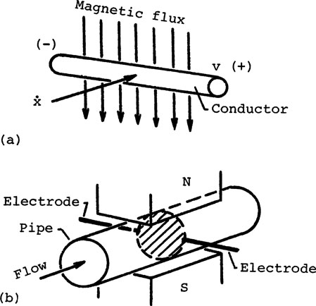
The basis of magnetic flowmeters is Faraday’s law of electromagnetic inductuion, which is the generator effect described in Chap. 5 (see Figs. 5-17 and 5-20). When a conductor moves with a transverse velocity $\dot{x}$ across a constantuniform magnetic field, as shown in Fig. 8-8a, the induced voltage υ is proportional to $\dot{x}$ of the conductor.

The schematic of a magnetic flowmeter shown in Fig. 8-8b consists of a moving conducting liquid in a magnetic field. The liquid at the cross section forms the conductor. The pipe section at the flowmeter must be non-magnetic to allow the magnetic flux to penetrate the pipe. The magnetic flux from north to south is generated by two coils laid on the pipe wall. Pulsed dc or ac can be used to power the coils. Electrodes are placed at points of maximum potential difference for a voltage output. The conducting path in the meter is a function of the conductivity of the liquid and the diameter of the electrodes.

FIGURE 8-8 Principle of magnetic flowmeter. (a) Electromagnetic induction. (b) Schematic of magnetic flowmeter.

The liquid must be conductive. The threshold is 10 μS/cm, where the unit siemens (S) is 1/ohm. For tap water, the conductivity is 200 μS/cm. Some liquids, such as gasoline, have low conductivity and are not appropriate for magnetic flowmeters. The conductivity of aqueous solutions is given in the literature [27]. Note that electrical conductivity may be a function of temperature, but it does not always increase with the solution concentration for some liquids.

Magnetic flowmeters are suitable for numerous applications. They are nonintrusive and have fast response. Forward and reverse flow can be measured with equal accuracy. The flow rate may range from 10⁻³ mm/s to high values. The lining for the pipe can be selected to accommodate the type of liquid. The meters are insensitive to viscosity, density, and type of flow conditions (turbulent or laminar) as long as the velocity profile is symmetrical. The operating characteristics of magnetic flowmeters can be obtained from manufacturers [28].

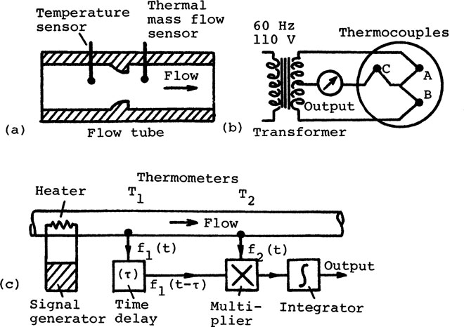
6.  Thermal Flowmeters

A thermal flowmeter uses temperature as its “tracer.” Since heat transfer to a flow stream is proportional to its mass flow rate, thermal flowmeters are basically mass flowmeters. Many methods of heat injection and signal extraction are used. For this discussion, these flowmeters are classifiedas being of heated tube or immersion type.

Thermal flowmeters are particularly useful for precision measurement of gases at low flow rates [29] from vacuum to high pressure when other types of meters are not suitable. Examples of applications are the measurement of low-velocity air in buildings and the accurate control of tungsten hexafluoride in the vacuum processing of semiconductors [30]. Within their design ranges, these flowmeters are relatively insensitive to changes in density, pressure, fluid viscosity, and temperature. As a thermal device, however, the response time of the meters is generally not high, but can be as short as 20 ms [31].

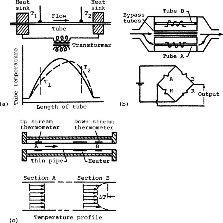
a. Heated-tube type. The mass flowmeter shown in Fig. 8-9a consists of a heated capillary tube and two heat sinks. The heat sinks keep the ends of the tube at the same temperature. The temperature profile is symmetrical (solid line) for zero flow, as shown in the figure. The flow causes an asymmetrical temperature profile (dashed line), and (T₂ – T₁) is a function of the mass flow rate. Note that this is another application of the deflection method (see Fig. 8-4c).

The laminar flowmeter shown in Fig. 8-9b consists of a sensor tube A and a reference tube B. A and B are exposed to an identical environment, but no flow occurs in B. Resistance thermal detectors RTDs can be used for both heating and temperature sensing. The flow is a function of the resistances of the RTDs, and the output is measured by means of a Wheatstone bridge. A range of 100:1 can be accomplished with this flowmeter. For low flow rates, only tube A is used. For high flow rates, tube A and the bypass tubes are used. Since the flow is laminar, the flow ratio between the sensor tube A and the bypass tubes is constant. Several flowmeters are based on variation of the same principle.

The boundary layer flowmeter shown in Fig. 8-9c is suitable for laminar and turbulent flow. It consists of a thin-walled pipe with temperature sensors, which are thermally insulated from each other. Assume that the thermal conductance of the pipe material is high and the heat loss to the surroundings is negligible. Heat is injected into the boundary layer of the fluid adjacent to the inner pipe wall, and the temperature profiles of the fluid at the sections are as shown in the figure. Heat transfer to the fluid depends on the surface film coefficient h of the boundary layer, and h is a function of mass flow rate. For a given fluid composition and design configuration, we have

FIGURE 8-9 Heated-tube mass flowmeters. (a) Deflection method (Model ST/STH Series Flowmeters. courtesy of Teledyne Hastings-Raydist, Hampton, Va.). (b) Laminar flowmeter (TMF Model 124, courtesy of Rosemont Engineering Co., Minneapolis, Minn.). (c) Boundary layer meter (from Ref. 32.

$\begin{array}{ll}Q=C_1{\dot{m}}^{0.8}\text{Δ}T\hfill & \text{for turbulent flow}\hfill \end{array}$

(8-16)

$\begin{array}{ll}Q=C_2{\dot{m}}^{1/3}\text{Δ}T\hfill & \text{for laminar flow}\hfill \end{array}$

(8-17)

where Q is the injected heat, C₁ and C₂are constants, m is the mass flow rate, and ΔT is the temperature difference.

b. Immersion type. The immersion-type mass flowmeter shown in Fig. 8-10a consists of two resistance thermal detectors RTDs in a flow tube. The heated RTD is the mass flow sensor. The unheated one is for temperature compensation. The resistance of the sensors form opposite arms of a Wheatstone bridge. The two RTDs may be packaged in a single probe (e.g., Series 100, Datametrics, Watertown, Massachusetts; FMA 300 Series, Omega Engineering, Stamford, Connecticut).

The flowmeter in Fig. 8-10b consists of two noble-metal thermocouples A and B in a low-voltage ac bridge circuit. The couples are heated by an ac current. The flow causes a change in the temperature of A and B and therefore a change in the dc output from the thermocouples. An identical unheated thermocouple C is placed in the dc metering circuit for temperature compensation. Note that the flowmeters in Fig. 8-10a andb use the same principle, consisting of a temperature sensor for the flow measurement and another for temperaturecompensation.

FIGURE 8-10 Immersion-type heat-transfer mass flowmeters, (a) Immersion type (Accu-Mass Series 370, courtesy of Sierra Instruments, Inc., Camel Valley, Calif.), (b) Heated thermocouples (Type K Flowtube, courtesy of Teledyne Hastings-Raydist, Hampton, VA.). (c) Cross-correlation of T₁ and T₂ (from Ref. 33).

A transit-time measurement using the cross-correlation technique is shown in Fig. 8-10c. The technique has general applications [34]. A train of heatpulses from a signal generator in a pseudo-random mode is injected into the field. Downstream are two fast-responding temperature sensors. The transit time detected by the sensors can be completely masked by noise. A cross-correlation function R₂₁(τ) measures the interdependency between f₁(t) and f₂(t) as a functionof the parameter τ, which is the time shift of one function with respect to the other [35].

$R_{21}\left(\text{τ}\right)={\displaystyle {\int }_{-\infty }^{\infty }{f}_2\left(t\right)f_1\left(t-\text{τ}\right)dt}$

(8-18)

As shown in the figure, (1) f₁(t) is shifted (delayed) by the time τ to become f₁(t – τ), (2) f₁(t – τ) and f₂(t) are multiplied, and (3) their product is integrated to yield an output. The process is repeated by varying the parameter τ. The correlated output peaks sharply when the delay time τ is equal to the transit time. The mathematical manipulations can be mechanized.

8-4.  INDIRECT FLOW MEASUREMENTS

As stated in the introduction, methods of flow measurements are classified as direct and indirect in this chapter. The basis of direct methods is the transport phenomenon of the fluid. The fluid itself is utilized to convey the flow information as it moves from one point to another in a flow stream.

An indirect method examines the effect of flow in a given flowmeasuring device, and the flow is measured by means of related physical quantities. In other words, an indirect method examines the flow and other physical quantities in a flow-related equation as prescribed by a physical law for the given problem. Any flow-related physical law can be utilized for a flow measurement.

The flowmeters described below are classified by the physical laws employed. For example, the square-root law, derived from Bernoulli’s equation, is the basis for a large class of flowmeters, and the flow is measured by means of a differential pressure. This includes orifices, venturi meters, flow nozzles, flow tubes, pitot-static tubes, and variable-area flowmeters. Turbine flowmeters operate on the momentum principle. Hot-wire and hot-film anenometers utilize the rate of convective heat transfer. Only commonly used flowmeters are described. It is evident that this study cannot be exhaustive.

8-5.  SQUARE-ROOT-LAW FLOWMETERS

The square-root-law flowmeter measures a fluid flow by means of a differential pressure, which is induced by placing an obstruction in the flow stream. This includes a large class of meters. They are generally designed for high Reynolds numbers.

The basis of the square-root law for incompressible flow is Bernoulli’s equation. Characteristics of square-root-law flowmeters will be examined after the description of a few examples. Bernoulli’s equation (Eq. 7-45) is modified to include the lost head h and to accommodate SI and English units.

$\frac{P_1-P_2}{\text{ρ}}{g}_c=\frac{V_2^2-V_1^2}{2}+g\left(Z_2-Z_1\right)+gh$

(8-19)

The equation shown has the dimensions (m/s)² or (ft/sec)².

P = absolute pressure	N/m2 (or Pa)	lbf/ft2
ρ = density	kg/m3	lbm/ft3
V = velocity	m/s	ft/sec
Z = elevation	m	ft
h = lost head	m	ft
g = acceleration due to gravity	9.807 m/s2	32.17 ft/sec2
gc = dimensional constant	1 kg · m/N · s2	32.17 lbm·ft/lbf·sec2

From continuity of flow, the theoretical volumetric flow rate Q_t is

$Q_t=A_{\text{1f}}{V}_{1\text{f}}=A_{2\text{f}}{V}_{2\text{f}}$

(8-20)

where the velocities V_1f and V_2f are measured at the fluid stream cross-sectional areas A_1f and A_2f, respectively. For an orifice, A_2f usually refers to the vena contracta or the minimum stream dimension. Neglecting the change in elevation and the lost head in Eq. 8-19, we get

$Q_t=\frac{A_{2\text{f}}}{{\left[1-{\left(A_{2\text{f}}/A_{1\text{f}}\right)}^2\right]}^{1/2}}{\left[\frac{2g_c\left(P_1-P_2\right)}{\text{ρ}}\right]}^{1/2}$

(8-21)

The theoretical volumetric flow rate Q_t is modified to obtain the actual flow rate Q_a.

$Q_a=\frac{C_d{A}_2}{{\left[1-{\left(A_2/A_1\right)}^2\right]}^{1/2}}{\left[\frac{2g_c\left(P_1-P_2\right)}{\text{ρ}}\right]}^{1/2}$

(8-22)

where A₁ is the internal cross-sectional area of a conduit, A₂ the flow area at the obstruction, and C_d the discharge coefficient. C_d = (actual flow rate)/(theoretical flow rate). Note that $1/{\left[1-{\left(A_2/A_1\right)}^2\right]}^{1/2}$ is a velocity of approach coefficient. It accounts for the change in cross-sectional areas of the flow stream. The discharge coefficient C_d accounts for losses in the flow process and the geometry of the setup, such as the nonoptimum location of pressure taps. The value of C_d for a given setup is mainly a function of Reynolds number N_R. Hence the results from the calibration with one fluid can be used for another.

Experimental values of C_d have been extensively investigated [36]. If a flowmeter is constructed according to certain standard dimensions, including the pressure tap locations, the value of C_d is predictable to within 1% for N_R > 10⁵. Although C_d is a function of N_R, it is relatively constant for certain design geometry of a flowmeter and N_R > 10⁴. The values of C_d, however, are sensitive to upstream flow disturbances caused by elbows, tees, valves, and so on. The error introduced may be as much as 15%. A rule of thumb is that a minimum run of 20 to 30 pipe diameters or straightening vanes must be used to smooth out the flow disturbances ahead of a flowmeter.

A.  Orifice and Venturi Flowmeters

1.  Orifice Meter

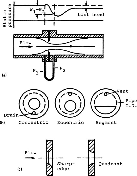
The sharp-edged orifice is commonly used because of its simplicity, low cost, and standardization. A sharp-edged orifice is a flat piece of metal with a hole machined to precise dimensions. Note that the standard design of a sharp-edged orifice requires that the edge be sharp and the plate be sufficiently thin relative to the diameter. Wear from long usage or abrasion may round off the upstreamedge of the orifice to cause a significant change in the value of its discharge coefficient C_d.

a. Incompressible flow. The flow pattern of a fluid in a concentric orifice is shown in Fig. 8-11a. The static pressure distribution and the permanent pressure loss (see Eq. 8-19) are as shown. Several schemes are used to locate the pressure taps, and the widely used flange taps are shown in the figure.

Three orifices are shown in Fig. 8-11b. The drain hole, when necessary, is for condensates in a gas flow, and the vent hole is for gases in a liquid flow. Eccentric and segment orifices are primary for liquids containing solids.

FIGURE 8-11 Orifices and flow patterns. (a) Flow pattern and pressure taps. (b) Orifices. (c) Profile of orifices.

The discharge coefficient C_d of an orifice is a function of Reynolds number N_R. The sharp-edged and quadrant orifices shown in Fig. 8-11c can be combined to give a constant C_d for N_R from 100 to 10⁴ [37]. The C_d of a sharp-edged orifice drops from 0.7 to 0.6 for this range. The quadrant orifice is developed to measure liquid flow with low Reynolds number. Its C_d rises from 0.7 to 0.9 for the same range. Hence a constant C_d can be obtained by using the two orifices in series or in parallel.

b. Compressible flow. Compressible flow is a study in thermodynamics [38]. The isentropic flow equation for orifices of an ideal gas is derived in this section [39]. The idealized conditions are zero heat transfer, mechanical work, mechanical friction, change in elevation, unrestrained expansion, and fluid turbulence. The last assumption is more appropriate for a venturi-type meter, since turbulence is unavoidable in an orifice.

The idealized pressure-volume relation of a gas is

$P{\upsilon }^k=\text{constant}$

(8-23)

where k is the ratio C_p/C_v of the specific heat, P the absolute pressure, and v the specific volume. For a one-dimensional compressible flow, the idealized energy balance equation is

$\frac{dP}{\text{ρ}}{g}_c+VdV=0$

(8-24)

where V is a velocity, ρ = 1/υ a density, and g_c a dimensional constant (g_c = 1 kg·m/N·s² or 32.17 lb_m·ft/lb_f·sec²). Substituting Eq. 8-23 into Eq. 8-24 and integrating, we obtain

$\frac{V_2^2-V_1^2}{2}=g_c\frac{k}{k-1}\left(\frac{P_1}{{\text{ρ}}_1}-\frac{P_2}{{\text{ρ}}_2}\right)$

(8-25)

For continuity, the mass flow rate is $\dot{m}={\rho }_1{A}_1{V}_1={\rho }_2{A}_2{V}_2$ where A₁ and A₂ are the areas of the flow sections. For circular sections, let the diameter ratio of the sections be $\beta ={\left({\text{A}}_{\text{2}}{\text{/A}}_{\text{1}}\right)}^{1/2}$. Combining these with Eq. 8-25, we obtain the theoretical mass flow rate ${\dot{m}}_t$

${\dot{m}}_t=\frac{A_2}{{\left[1-{\text{β}}^4{\left(P_2/P_1\right)}^{2/k}\right]}^{1/2}}{\left\{2g_c\frac{k}{k-1}{P}_1{\text{ρ}}_1\left[{\left(\frac{P_2}{P_1}\right)}^{2/k}-{\left(\frac{P_2}{P_1}\right)}^{\left(k+1\right)/k}\right]\right\}}^{1/2}$

(8-26)

The equation is multiplied by an appropriate discharge coefficient C_d to obtain the actual flow. The same C_d can be used for liquid and gas flow having the same Reynolds number. Note that the simpler incompressible flow equation, (Eq. 8-22), is often used for compressible flow at low velocities. An investigation of the error due to the simplification is given as an exercise.

There is a lack of basic references for measuring the flow of compressible fluids. The properties of a fluid, such as pressure and temperature, are more variable for a compressible flow. Different types of meters for compressible flow can give different results in a field test with the meters on the same line [40].

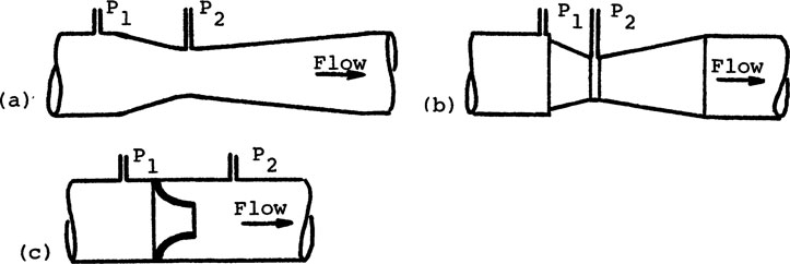
2.  Venturi, Dall Flow Tube, and Flow Nozzle

The venturi meter shown in Fig. 8-12a has a smooth entrance and exit cone, like a convergent-divergent nozzle. It has a well-formed streamlined flow. The Dall flow tube in Fig. 8-12b is similar to a venturi. The flow nozzle in Fig. 8-12c does not have an exit cone. These meters can handle large flows at high Reynolds number N_R. They cost more than orifices, occupy more space, and are not easily removed from the line for inspection.

Due to the more complex geometry, these flowmeters are less standardized compared with sharp-edge orifices and are calibrated individually. The discharge coefficient C_d of a venturi and a flow nozzle ranges from 0.94 at N_R = 10⁴ to 0.99 at N_R = 10⁶. The C_d of a Dall tube is about 0.67, like that of an orifice.

Flow nozzles have less permanent lost head than do orifices (see Fig. 8-11). Dali flow tubes have the least head loss among these meters. The lost head is an energy cost in pumping. The energy cost of an orifice is about $900 per year for an industrial setting [41]. The total cost, of course, must include many items, such as the initial cost, startup, and maintenance.

B.  Characteristics of Square-Root-Law Flowmeters

Characteristics of the square-root-law or “obstruction” type flowmeters are briefly examined. Their range is limited because the flow rate is proportional to the square root of the differential pressure for the flow measurement. If the readable range of (P₁ – P₂) is 16:1, the range of the flow rate is only 4:1.

The meter is more sensitive and therefore more accurate for higher flow rates than for lower flow rates, since (P₁ – P₂) is proportional to Q² and ΔP/ΔQ is larger for higher flow rates. For consistent accuracy, the error should be a constant percentage of the flow. By the same token, the error in a total flow for the same meter is also a function of its flow rates. For example, the total flow over a time interval is the integral of flow rates. If the total flow is mainly from low flow rates, accuracy cannot be improved by integrating over a longer interval.

Error in flow rates for pulsating flow is somewhat controversial. An experimental study shows that the pulsating flow of incompressible fluids can be accurately metered with orifices if the time average of the square root of ΔP is determined [42]. It is erroneous to use the square root of the time average of ΔP. This is expressed in the inequality

FIGURE 8-12 Flowmeters. (a) Venturi. (b) Flow tube. (c) Flow nozzle.

$\frac{1}{T}{\displaystyle {\int }_0^T{\left(\Delta P\right)}^{1/2}dt\ne {\left(\frac{1}{T}{\displaystyle {\int }_0^T\Delta Pdt}\right)}^{1/2}}$

(8-27)

In other words, the average should be based on the square-root law, but noton the average of the differential pressure. This seems self-evident, because the change in flow rate is larger for a +ΔP than for a −ΔP. Hence an average differential pressure tends to give a larger flow rate.

The accuracy of an orifice meter also depends on its physical dimensions [43]. Assuming that there is no change in ΔP and fluid properties, it can be shown from Eq. 8-22 that

$\frac{\Delta Q}{Q}=\frac{\Delta C_d}{C_d}+\frac{2}{1-{\text{β}}^4}\frac{\Delta d_2}{d_2}-\frac{2{\text{β}}^4}{1-{\text{β}}^4}\frac{\Delta d_1}{d_1}$

(8-28)

where β = d₂/d₁ is a ratio of the diameter of the orifice and the pipe. The error ΔC_d/C_d may be due to changes in flow conditions or an erosion of the sharp edges of an orifice. The error Δd₂/d₂ due to the diameter of the orifice, however, may dominate the overall error in a measurement.

C.  Pitot-Static Tubes

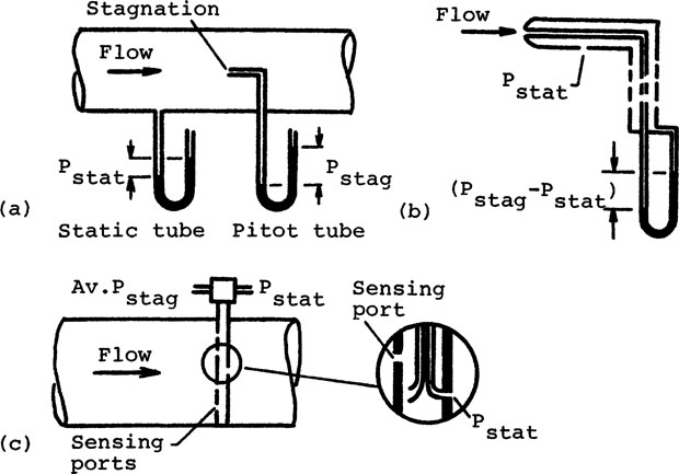
A pitot-static tube measures the local velocity of a flow instead of an average flow as in flowmeters. The pitot or impact tube shown in Fig. 8-13a is a tube with one end bent at a right angle toward the flow direction. The flow stagnates at the impact tube. The difference between the stagnation and static pressure is used to indicate the local velocity of a free stream.

FIGURE 8-13 Pitot-static tubes. (a) Pitot and static tube. (b) Pitot-static tube. (c) Annubar.

The pitot-static tube as a single unit is shown in Fig. 8-13b. The annubar [41] shown in Fig. 8-13c measures the average stagnation pressure across a pipe section by means of a number of sensing ports. It measures the average flow rate across a pipe without the penalty of high lost head as in orifices.

1.  Incompressible Flow [44]

The basis of the pitot-static tube is the square-root law. From Eq. 8-19, P₁ is the static pressure P_s of the undisturbed free stream at the velocity The fluid is brought to rest (V₂ = 0) isentropically at stagnation. Hence the stagnation pressure is the total pressure P_t (= P₂) due to P_s and the velocity V₁. From Eq. 8-19 we get

$V={\left[\frac{2g_c}{{\text{ρ}}_{\text{stat}}}\left(P_t-P_S\right)\right]}^{1/2}$

(8-29)

The static pressure is usually more difficult to measure. The equation can be modified by a calibration constant if the static pressure indicated is not the true value. A correction is not necessary in a Prandtl pitot-static tube [45].

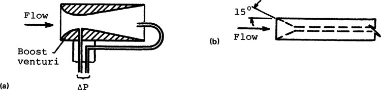
A pitot-static tube becomes insensitive at low velocities. A larger ΔP signal can be obtained by means of a boost venturi, as shown in Fig. 8-14a, but the P_s is no longer that of the free stream. Error in the total pressure due to a misalignment depends on the geometry of the impact tube. The square-ended tube with a 15° internal bevel angle shown in Fig. 8-14b is capable of providing total pressure data with errors of less than 1% if the misalignment with the flow stream is less than 25°.

FIGURE 8-14 Configurations of pitot-static tubes. (a) Pitot-static tube. (b) Pitot tube.

2.  Compressible Flow

The free-stream velocity V for compressible flow is obtained by substituting Eq. 8-23 into Eq. 8-25. Letting V₁ = V, V₂ = 0, P₁ = P_s, P₂ = P_t, and simplifying, we get

$V={\left\{\frac{2g_{c}k}{k-1}\frac{P_s}{{\text{ρ}}_{\text{stat}}}\left[{\left(\frac{P_t}{P_s}\right)}^{\left(k-1\right)/k}-1\right]\right\}}^{1/2}$

(8-30)

In gas dynamics, Eq. 8-30 is usually expressed in terms of Mach number N_M of the free stream, where N_M = V/c and $c={\left(kP/\rho \right)}^{1/2}$ is the sonic velocity. Thus Eq. 8-30 can berewritten as

$P_t=P_s{\left(1+\frac{k-1}{2g_c}{N}_{\text{M}}^2\right)}^{k/\left(k-1\right)}$

(8-31)

For supersonic flow (N_M > 1), a shock wave is formed ahead of the pitot tube. Velocity calculations for this case is beyond the intended scope of this book.

D.  Variable-Area Flowmeters

A variable-area flowmeter may have a fairly wide working range. For the meters described above, such as a flow orifice, the area of the obstruction is fixed, and the differential pressure changes with flow rate. For a variable-area meter, the area of the obstruction changes with flow rate, but the differential pressure generally remains constant.

1.  Flow Indicators

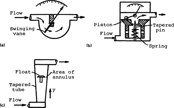
A flow indicator with a swinging vane is shown in Fig. 8-15a. A spring load (not shown) closes the meter for zero flow. An increasing flow forces the vane to rotate, thereby providing a larger area for the flow. The flow indicator shown in Fig. 8-15b changes the flow area between a taper pin and a fixed-size orifice in a spring-loaded piston. An increasing flow forces the piston to rise, thereby increasing the annular area between the pin and the orifice.

2.  Rotameter

Rotameters are commonly used for medium flow rates and for visual flow indications. Their working range is 10:1 instead of 4:1 as described above. They can also be used for very small flow rates, of the order of 0.05 cm³/min for liquids and 2 cm³/min for gases [46]. The accuracy is about 2%.

The rotameter shown in Fig. 8-15c consists of a float and a vertical transparent tapered tube with graduations along its axial direction. The tube diameter is larger at the top than the bottom. Fluid enters from the bottom of the tube, passes upward through the annulus between the float and the tube, and exits through the top. For a given flow rate, the float assumes an equilibrium position y to indicate the flow rate. The float may be spherical or cylindrical. It may be shaped to obtain particular effects, such as to induce turbulence in the flow to minimize the effect of viscosity.

FIGURE 8-15 Variable-area flowmeters, (a) Swinging-vane meter (Series LL and LG, courtesy of Universal Flow Monitors, Hazel Park, Mich.). (b) Taperedpin meter (Series W, courtesy of Universal Flow Monitors, Hazel Park, Mich.). (c) Rotameter.

When the float is at equilibrium, the vertical forces due to differential pressure, viscosity, buoyancy, and gravity are balanced. A simplified model assumes that the downward force due to gravity minus buoyancy is equal to the upward force due to the differential pressure across the float. Thus a force balance on the float gives

$A_F\text{Δ}P={\text{Vol}}_F\left({\text{ρ}}_F-\text{ρ}\right)\frac{g}{g_c}$

(8-32)

where

A_F = projected area of the float

ΔP = differential pressure across the float

Vol_F = volume of the float

ρ_F = density of the float

ρ = density of the fluid

g = acceleration due to gravity

g_c = dimensional constant (see Eq. 8-19)

The volumetric flow rate Q_a is obtained by substituting ΔP for (P₁ – P₂) from Eq. 8-32 into Eq. 8-22:

$Q_a=\frac{C_d\left(A_T-A_F\right)}{{\left\{1-{\left[\left(A_T-A_F\right)/A_T\right]}^2\right\}}^{1/2}}{\left[\frac{2{\text{Vol}}_F\left({\text{ρ}}_F-\text{ρ}\right)g}{\text{ρ}{A}_F}\right]}^{1/2}$

(8-33)

where C_d is the discharge coefficient, A_T the cross-sectional area of the tapered tube at the float, and A_T – A_F the annular flow area. Hence A_T = A₁ and A_T – A_F = A₂.

Q_a is approximately linear with the float position y when the variation in C_d is small, the fluid density ρ is constant, and the tube is shaped that the annular area A_T – A_F = Ky, where K is a constant. Since [(A_T – A_F)/A_T]² is always much less than 1, we obtain the approximate equation

$Q_a\simeq \left(\text{constant}\right)y$

(8-34)

If the density of the float to that of the fluid is 2:1, the same meter can be used to measure the mass flow rate of any fluid [47]. Mass flow rate is the product of Q_a and the fluid density ρ. Assume that A_T – A_F ≃ Ky and {1 – [(A_T – A_F)/A_T]²}^1/2 ≃ 1. From Eq. 8-33, the mass flow rate is

$\dot{m}=C_{1}y{\left[\text{ρ}\left({\text{ρ}}_F-\text{ρ}\right)\right]}^{1/2}$

(8-35)

where C₁ is constant. The differential $d\left(\dot{m}/y\right)/d\rho$ gives

$\frac{d\left(\dot{m}/y\right)}{d\text{ρ}}=\frac{C_2\left({\text{ρ}}_F-2\text{ρ}\right)}{{\left[\text{ρ}\left({\text{ρ}}_F-\text{ρ}\right)\right]}^{1/2}}$

(8-36)

where C₂ is constant. The condition for $\dot{m}/y$ independent of the fluid densityρ is

${\text{ρ}}_F=2\text{ρ}$

(8-37)

E.  Drag-Force Flowmeters

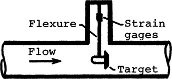
The drag-force or target flowmeter shown in Fig. 8-16 consists of a drag body immersed in a flow stream and a flexture with strain gages to indicate the drag force due to the flow. The drag force on the immersed body is

$F=CA\frac{\text{ρ}{V}^2}{2g_c}$

(8-38)

where

F = drag force on the body

C = nondimensional drag coefficient

A = target area

ρ = fluid density

V = free-stream velocity

g_c = dimensional constant

The volumetric flow rate is the product of V and the free-stream cross-sectional area. For sufficient high Reynolds number and properly shaped body [48], C is fairly constant. The flowmeter is also governed by the square-root law, since the velocity V is proportional to the square root of the drag force F.

The meter is bidirectional if the drag body is symmetrical. The flow measured is independent of pressure and temperature when the value of C and the fluid density ρ are reasonably constant. The flexure-and-drag body is a lightly damped second-order system. Hence one advantage of the meter is its high frequency response.

FIGURE 8-16 Drag-force (target) flowmeter.

8-6.  TURBINE FLOWMETERS

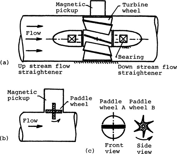
A turbine-type flowmeter works on the momentum principle. It consists of a free-running small turbine suspended in a pipe. The rotation speed of the turbine is proportional to the velocity of the fluid, similar to the familiar anemometer for wind velocity measurements. Since the flow area of the meter is fixed, the rotational speed is proportional to the volumetric flow rate.

The turbine flowmeter shown in Fig. 8-17a consists of a straight pipe, a free-running multibladed turbine wheel on bearings, the upstream and downstream flow straighteners (not shown), and a pickup outside the fluid passage. Generally, an installation requires a minimum of 10 diameters of straight pipe upstream and five downstream.

The pickup gives one voltage pulse for each blade passing the pickup.

FIGURE 8-17 Turbine flowmeters. (a) Turbine flowmeter. (b) Paddle-wheel flowmeter. (c) Paddle wheels.

Thus the flow rate or the total flow is measured by counting. The pulse output is a convenience for digital control. A magnetic pickup is commonly used (see Fig. 5-20a). The magnetic drag on the turbine wheel will degrade the linearity of the meter at low flow rates, but this can be compensated by using a carrier type system.

Turbine flowmeters are commonly used. Since the operation is not based on the square-root law, the range is about 10:1 instead of 4:1. They are available in sizes from ⅛ to 8 in. in diameter, and are used for many type of fluids for a wide range of pressure and temperature. The effect of viscosity is secondary within the linear range. The pressure drop across a meter is about 3 to 10 psi. The accuracy is about 0.1% for liquids and 0.5% for gases with excellent repeatability. With a low-inertia rotor, the meter has good dynamic response, although it always reads high for pulsating gas flows [49].

In addition to the advantages above, these flowmeters are relatively maintenance free. A limitation is the bearing wear. Since the meter has a large range, an oversized flowmeter should be selected to prolong bearing life and to avoid damage to the meter due to overspeeding.

The paddle-wheel type shown in Fig. 8-17b is less expensive. The accuracy is about 2%, but the same transducer can be used for a limited range of pipe sizes. Two designs for paddle wheels, labeled A and B, are shown in Fig. 8-17c.

8-7.  VORTEX-SHEDDING FLOWMETERS

Vortex-shedding and swirl flowmeters are described in this section. The flow of fluid around solid bodies is studied extensively [50]. Vortex-shedding flowmeters are based on the von Karman effect. These meters were introduced in the late 1960s. They have gained wide acceptance, and their applications are studied actively [51].

Vortices or eddies shed alternately from a body immersed in a fluid at a steady flow, and the vortices travel downstream with the flow. The frequency of the shedding is given by the Strouhal number N_S, which is a function of Reynolds number N_R:

$N_{\text{S}}=\frac{fD}{V}=\varphi \left(N_R\right)$

(8-39)

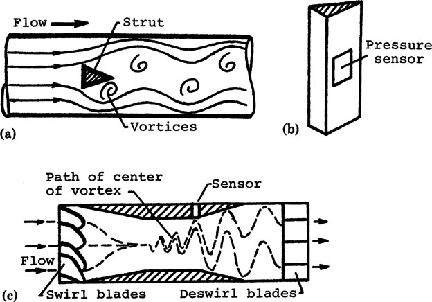
where f is the shedding frequency, D a characteristic dimension of the shedding body, and V the fluid velocity. For the triangular bluff body or strut shown in Fig. 8-18a, N_S is reasonably constant for 10⁴ < N_R < 10⁶. Within this range, the frequency of shedding is directly proportional to the fluid velocity and therefore the volumetric flow rate. Note that the output signal is the shedding frequency rather than the magnitude of the vortices.

FIGURE 8-18 Flowmeters based on fluid oscillations. (a) Vortex shedding. (b) Triangular strut. (c) Swirlmeter.

Many schemes are used to count the shedding frequency. Since the vortices cause local pressure pulses to alternate on the shedder, the frequency signal can be sensed by a pressure transducer. The frequency signal can also be detected by means of the turbulence from the vortices, which are at regular intervals. An ultrasonic, laser Doppler, or a resistance thermal detector RTD-type sensor can all be employed for this purpose.

Many bluff bodies are used to produce vortex shedding. Two bluff bodies of radical different shapes could be identical vortex shedders if their Strouhal numbers were identical. In fact, the same calibration of a meter can be used for both liquid and gas. This “universal” design simplifies calibration, maintenance, and the interchanging of parts. A triangular strut with provision for pressure sensing is shown in Fig. 8-18b. In some meters, a second strut can be used for the hydrodynamic amplification of the vortex shedding (e.g., DV Series, Fisher Controls, St. Louis, Missouri).

Accuracy of vortex-shedding flowmeters is about 0.5% of reading with excellent repeatability. The working range is 20:1 and a linear range of 100:1 is attainable. Upstream and downstream straight piping are necessary for proper installation. The meter can be used for a wide range of fluids, but slurries or high-viscosity liquids are not recommended.

The main advantages of vortex-shedding flowmeters are no moving parts, good accuracy with long-term repeatability, large operating range, linear output with reasonable lost head, suitable for gas or liquid, and calibration not affected by viscosity, density, pressure, or temperature. It is cost-effective compared with many common flowmeters. The main sources of error are turbulent eddies carried into the meter, mechanical vibration, and sound waves in the fluid.

The swirlmeter [52] shown in Fig. 8-18c also uses oscillations of a fluid for velocity measurement, but employs the vortex precession principle instead of vortex shedding. It has no moving parts. The swirl traces a helical path through the flow. The pitch of the helix is fixed by the meter, but the rate at which the helix passes a point is proportional to the volumetric flow rate. The operation is analogous to the threads of a screw which travel in accord with the rate of rotation. The signal can be sensed by a thermister or a RTD-type transducer.

8-8.  HOT-WIRE AND HOT-FILM ANEMOMETERS

Hot-wire anemometers have been used since the late nineteenth century. The hot-film type is more rugged and is a recent introduction. Constant-temperature and constant-current hot-wire anemometers are described in this section. The latter has largely been replaced by the constant-temperature type.

The instrument is based on the convective heat transfer from a heated sensor to its surrounding fluid. The heat loss depends on the fluid velocity, temperature, pressure, density, and thermal properties, as well as the temperature and physical parameters of the sensor. Since these are potential noise inputs in a measurement, they also show potential applications of the instrument (see Eq. 2-4). Literature on th subject is extensive [53]. A basic text by Lomas [54] is well worth reading.

Hot-wire anemometers are used mainly to measure rapid fluctuating velocities in gas and liquid. The instrument has excellent frequency response and an upper frequency limit of 400 kHz is commercially available. Among the flowmeters described in this chapter, only the laser Doppler velocimeter is comparable in this performance.

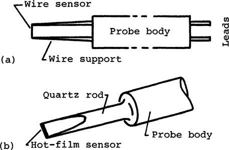
The probe of a hot-wire anemometer, shown in Fig. 8-19a, consists of a fine-wire sensor, the wire supports, a probe body, and electrical leads. The wire is about 1 mm (40 × 10^–3 in.) in length and 5 μm (0.2 × 10^–3 in.) in diameter. Tungsten, platinum, and platinum alloys are used for the wire. The sensor of a hot-film probe, shown in Fig. 8-19b, is usually made of platinum deposited in a thin layer onto a substrate of fused quartz.

FIGURE 8-19 Probes for hot-wire and hot-film anemometers. (a) Hot-wire probe. (b) Wedge hot-film probe.

The energy balance of a heated wire at equilibrium is

$\underset{\begin{array}{l}\text{power}\\ \text{input}\end{array}}{\underbrace{I^{2}R}}=\underset{\begin{array}{l}\text{Convective}\text{heat}\\ \text{transfer}\end{array}}{\underbrace{hA\left(T-T_f\right)}}$

(8-40)

where I is an electric current, R the wire reistance, h the heat transfer film coefficient, A the heat transfer area, and T and T_f are the wire and fluid temperatures. The heat transfer from a cylinder ofinfinite length is commonly expressed in King’s law:

$h={C^{\prime }}_1+{C^{\prime }}_2{\sqrt{N}}_R$

(8-41)

or

$h=C_1+C_2{V}^n$

(8-42)

where the C’s are parameters [55], N_R is the Reynolds number, V the fluid velocity, and n ≃ 0.5. The resistance R of a hot-wire sensor is

$R=R_0\left[1+\text{α}\left(T-T_0\right)\right]$

(8-43)

where R₀ is the resistance at the reference temperature T₀, and α the coefficient of resistivity. Thus the temperature of a wire can be measured by means of its resistance.

A. Constant-Temperature Anemometers

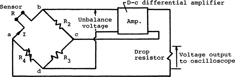
The simplified circuit of the constant-temperature anemometer shown in Fig. 8-20 consists of bridge circuit and a high-gain dc differential amplifier in a feedback loop. Let the bridge be initially balanced with zero excitation and fluid velocity V. The bridge is unbalanced by increasing R₄ and keeping V = 0. Thus the voltage across b-d is the unbalance input to the amplifier. This increases the excitation voltage to the bridge across a-c and the current I through the sensor. Subsequent increase in temperature and resistance R of the sensor reduces the unbalance voltage. The process is self-adjusting. An equilibrium is reached when the imbalance voltage becomeszero and the sensor is at a desired temperature. The differential temperature (T – T_f) in Eq. 8-40 is typically maintained at about 450°F in air and 80°F in water. This gives the reference current I₀.

A fluid flow cools the sensor, decreases its resistance R, and unbalances the bridge. Since the feedback loop is self-adjusting, it automatically increases the excitation to the bridge to restore the balance. The velocity V of the fluid can be measured by means of the voltage across the terminals a and c at the bridge. Alternatively, a drop resistor can be inserted to measure the total current to the bridge as shown in the figure. Assuming n ≈ 0.5in Eq. 8-40, it can be shown that

$V=C_0{\left[{\left(\frac{I}{I_0}\right)}^2-1\right]}^2$

(8-44)

where C₀ is a calibration constant and I₀ the current through the sensor to give the desired temperature for V = 0. An anemometer is calibrated by exposing the probe to a known velocity in the fluid in which it is to be used.

FIGURE 8-20 Constant-temperature anemometer with feedback.

B.  Constant-Current Anemometers

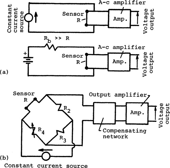
Feedback is not used for constant-current anemometers. The circuits for the constant-current drive in Fig. 8-21a are the basic circuits presented in Sec. 3-5 (see Figs. 3-36b and 3-37b). A constant-current source can be replaced by a constant-voltage source with a high series resistance R_b(R_b = 2 kΩ and R = 1 Ω.

The frequency response of the anemometer in Fig. 8-21a is only about 160 Hz [56]. This can be deduced from the time constant of the sensor in an energy balance equation, similar to finding the time constant of a thermometer (see Prob. 4-2). The frequency response can be improved by means of series compensation as shown in Fig. 8-21b (see Fig. 4-30). The time constant of the sensor, however, is unknown, and the scheme for obtaining the correct compensation involves additional circuitry [57].

FIGURE 8-21 Constant-current anemometer circuits. (a) Velocity fluctuation measurement. (b) Anemometer with compensation.

Hot-wire instruments are sensitive and versatile. They are available in numerous configurations [58] for specific applications. However, they are delicate instruments and must be used properly. Breakage and burnout are not uncommon. An unexpected flow reversal in the vicinity of the probe may be interpreted as an decrease in velocity followed by an increase. Some conditions that may cause difficulties are misalignment, probe fouling, sensor aging, conducting liquids such as mercury [59], low-velocity measurements, air bubbles in the liquid, vortex shedding from parts of the probe, and hydrodynamic interference from another probe or a nearby object.

8-9.  MASS FLOWMETERS

Mass flowmeters are used when a product is sold by weight or when the performance of a machine is based on mass measurements, such as a liquid-fueled rocket engine. The mass flow rate of a fluid can be obtained from the product of its density and volumetric flow rate. This is an indirect method and commonly used, but the density measured at one location is not always that at the flowmeter, such as in cryogenics [60]. Mass flow rate can also be measured directly. Examples of both methods are described in this section.

A.  Density Measurements

Density measurements as an intermediate step for finding mass flow rates are described in this section. Some instruments must be compensated for effects of flow, pressure, temperature, or viscosity.

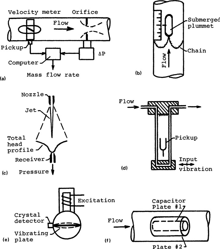
The turbine-orifice combination shown in Fig. 8-22a measures the fluid velocity V and the ΔP across the orifice. Since V is determined, the density ρ can be deduced from Eq. 8-22. The submerged plummet in Fig. 8-22b is a “hydrometer.” A change in density changes the effective weight of the plummet and chain. The jet and the coaxial receiver shown in Fig. 8-22c are separated by a fixed distance. Clean air is supplied to the jet. The pressure detected at the output is a measure of the gas density between the jet and the receiver. The density of a flowing liquid is measured as shown in Fig. 8-22d, in which the resonant frequency of the liquid-filled pipe is sustained by means of feedback. A density change in the liquid causes a change in resonant frequency. Similarly, a vibrating plate is used in the densitometer shown in Fig. 8-22e. The resonant frequency of a plate immersed in a confined volume changes with the density of the surrounding fluid. The capacitance between the coaxial plates shown in Fig. 8-22f changeswith the dielectric constant of the fluid, which is a function of its density. Dielectric densitometers are used for flowmetersin cryogenics.

FIGURE 8-22 Techniques for density measurement. (a) Indirect method. (b)“Hydrometer.” (c) Jet pressure (Model 601D, Turbojet Densitometer. courtesy of Fluid Dynamic Devices Ltd., Mississauga, Canada). (d) Resonant frequency. (e) Vibrating plate. (f) Dielectric “constant.”

The examples above show that any density-related equation can be used for a density measurement. Some equations feasible for density measurements are

$I=I_0{e}^{-\text{μ}d}$

(8-45)

$c=\sqrt{\frac{kP}{\text{ρ}}}$

(8-46)

$\text{ρ}=\frac{P}{RT}$

(8-47)

The nuclear-radiation absorption coefficient μ of a material is proportional to its density. It is feasible to use radiation attenuation in Eq. 8-45 for density measurement, where the I’s are radiation intensities and d is the separation between the radiation source and detector. The density ρ of a gas in Eq. 8-46 is related to the sonic velocity c, pressure P, and specific heat ratio k (= C_p/C_v). The gas law in Eq. 8-47 relates the density ρ, absolute pressure P, absolute temperature T, and gas constant R.

B.  Direct Mass Flowmeters

A true mass flowmeter should be independent of other physical variables of the fluid, the type of flow, and ambient conditions. The simplest method is to determine the mass flow rate by weighing (see Fig. 8-2), but this is not always convenient in field applications. Thermal flowmeters (see Figs. 8-9 and 8-10) are basically mass flowmeters, provided that the specific heat remains constant. Examples of direct mass flowmeters are described in this section.

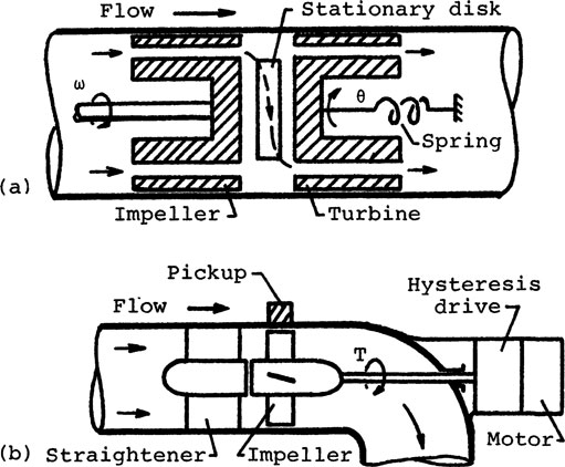
Angular momentum principle is used in the direct mass flowmeter shown in Fig. 8-23a. It consists of an impeller driven at a constant angular velocity ω, a stationary disk to decouple the viscosity effect of the fluid, a turbine for the momentum transfer, and a torsional spring to restrain the turbine from free rotation. The impeller gives a swirl or an angular momentum to the flowing fluid. The swirl is removed by the turbine. From Newton’s second law, the torque T on the turbineis

$T=\frac{d}{dt}\left(J\omega \right)$

(8-48)

or

$T=\text{ω}{k}^2\frac{dm}{dt}$

(8-49)

where J is the mass moment of inertia of the fluid of mass m, ω a constant angular velocity of the motor, and k the radius of gyration of the fluid mass m. For constant ω and k, the torque T indicated by the spring is proportional to the mass flow rate dm/dt. The range of the meter is 10:1 for constant flow rates. Under unsteady flow conditions, the viscous force in the system may become large.

FIGURE 8-23 Momentum-type mass flowmeters. (a) Constant-co impeller/turbine meter (courtesy of General Electric Aerospace Div., Wilmington, Mass.). (b) Constant-torque impeller meter.

The mass flowmeter shown in Fig. 8-23b works on the same principle. It consists of an impeller, a motor, and a hysteresis drive (similar to a slip clutch) to give a constant torque T. The constant T can also be maintained by means of a servo system. For T and k constant in Eq. 8-49, the mass flow rate dm/dt is proportional to 1/ω. If a magnetic pickup is used to measure the speed, the time interval At between pulses from the pickup is inversely proportional to ω. Hence dm/dt is linear with Δt. The meter has high resolution at low flow rates, but the resolution decreases at higher flow rates.

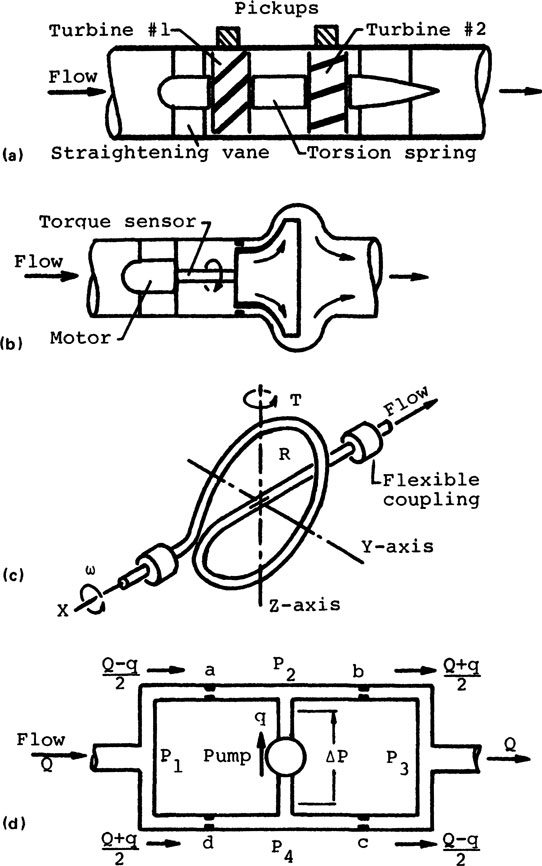
Variations of the momentum principle are used in other mass flowmeters. The design shown in Fig. 8-24a consists of two free-running rotors coupled through a torsional spring. Each rotor has a different pitch angle for its blades. The spring allows the rotors to rotate at the same speed but out of phase with one another. The mass flow rate is proportional to the relative angular displacement between the rotors. The “Coriolis” meter shown in Fig. 8-24b measures mass flow rate by means of the torque required to maintain a constant angular velocity in the fluid while it moves radially. The fluid in the gyroscopic mass flowmeter shown in Fig. 8-24c is forced through a 360° loop while the loop is rotating about the X axis at a constant angular velocity. The precession moment produced about the Z axis is proportional to the mass flow rate. This is measured at the flexible couplings shown in the figure.

FIGURE 8-24 Mass flowmeters. (a) Twin-turbine mass flowmeter. (b) Coriolis mass flowmeter (from Ref. 61). (c) Gyroscopic mass flowmeter. (d) Bridge-circuit mass flowmeter (courtesy of Flo-Tron, Inc., Paterson, N.J.).

A differential pressure bridge as a mass flowmeter is shown in Fig. 8-24d. It consists of a bridge with four identical orifices and a positive-displacement pump at a constant flow rate q. Liquid at a volumetric rate Q is supplied to the meter. Assume that q < Q. The flow through the orifices are as shown in the figure. The flow and pressure drop across orifice a and orifice d are

$\begin{array}{lll}\frac{Q-q}{2}=C\sqrt{\frac{P_1-P_2}{\text{ρ}}}\hfill & \text{and}\hfill & \frac{Q+q}{2}=C\sqrt{\frac{P_1-P_4}{\text{ρ}}}\hfill \end{array}$

(8-50)

where C’s are constants. Combining the equations and simplifying, the mass flow rate ρQ is

$\text{ρ}Q=\frac{C}{q}\left(P_2-P_4\right)=k\left(P_2-P_4\right)$

(8-51)

where k = C/q is a constant. It can be shown that the mass flow rate ρQ is proportional to (P₁ – P₃) for q > Q. The operation of the meter is independent of pressure, temperature, and density of the liquid, but the density must remain unchanged within the meter. Hence the meter is suitable only for liquids. Its range is from 30:1 to 100:1 with accuracy of 0.5% of reading. These flowmeters are available from 0.1 to 50,000 lb_m/hr.

PROBLEMS

  8-1.  Water flows in a 4-in.-diameter pipe with an average velocity of 15 ft/sec. The temperature is T = 80°F, density ρ = 62.2 lb_m/ft³, and viscosity μ = 1.77 × 10⁻⁵ lb_rsec/ft². (a) Calculate the Reynolds number, (b) Convert the data into SI units and verify the answer.

  8-2.  The on-line measurement of the viscosity of a fuel oil is as shown in Fig. 7-33e. The apparatus consists of a temperature-controlled tubing (L = 25 cm and D = 4 mm) and a constant-delivery pump. Calculate the absolute viscosity if the average velocity of the flow is V = 1.5 m/s, the differential pressure across the tubing (P₁ – P₂) = 2.5 kPa, temperature T = 40°C, the specific gravity is 0.90, and the density of water is 992 kg/m³.

  8-3.  A model study is proposed for airflow in a 1.0-m-diameter duct with a gage pressure of 10 kPa and an average velocity of 10 m/s. Select one of the models below and give your reasons for the selection. (a) Airflow in a 10-cm-diameter pipe. (b) Water flow in a 6-cm-diameter pipe. (c) Oil flow in a 6-cm diameter pipe.

 Data (at atmospheric pressure):

	Absolute viscosity (Pa · s)	Kinematic viscosity (m2/s)
Air	1.78 × 10–5	1.49 × 10–5
Water	1.08 × 10–3	1.08 × 10–6
Oil	3.75 × 10–3	4.38 × 10–6

  8-4.  The drag force F on a submerged body is a function of the fluid density ρ, absolute viscosity μ, velocity V, and a characteristic dimension D. Use dimensional analysis (a) to And the dimensionless ratio of F and μ, and (b) to show that the force coefficient is a function of Reynolds number N_R.

  8-5.  The accuracy of a lobed-impeller meter (see Fig. 8-3f) for volumetric airflow from 1000 to 4000 ft³/min is ±1%. If the air pressure is (20.0 ± 0.2) psia and temperature is (120 ± 2)°F, calculate the uncertainty in the mass flow rate.

  8-6.  Show a sketch of the ASME recommended proportions for each of the obstruction meters and give reference(s) for the information: (a) sharp-edged orifice; (b) venturi tube; (c) long-radius flow nozzle.

  8-7.  Show a plot of the discharge coefficient C_d versus Reynolds number N_R for each of theobstruction meters and give reference(s) for the information: (a) sharp-edged orifice; (b) venturi tube; (c) long-radius flow nozzle.

  8-8.  A sharp-edged concentric orifice is used to measure the flow of water in a 10-cm-diameter pipe. The diameter ratio of orifice to pipe is 0.40 and the differential pressure is 100 kPa. (a) Calculate the flow in gallons per minute. Data: Density ρ = 997 kg/m³, viscosity μ = 8.94 × 10⁻⁴ Pa.s, C_d = 0.61,1 gallon = 3.786 × 10⁻³ m³. (b) Convert the data to SI units and verify the calculations.

  8-9.  A venturi for metering fuel oil is calibrated as shown in Fig. 8-2a. Pipe diameter D₁ = 4 in. and D₂:D₁ = 0.5:1. The flow rate is 500 gal/min. (a) Calculate its discharge coefficient C_d. Data: oil specific gravity = 0.86, μ = 6.02 lb_f·sec/ft², water density = 62.4 lb_m/ft³, ΔP = 15 psi. (b) Convert the data into SI units and verify the calculations.

8-10.  The flow of a heavy oil through a 20-cm-diameter pipe at 3000 barrels per hour is measured by means of a sharp-edged concentric orifice, (a) Calculate the pressure drop across the orifice and estimate the power requirement. Data: temperature T = 40°C, density ρ = 892 kg/m³, viscosity μ = 0.0521 Pa·s, C_d = 0.62, diameter ratio (orifice):(pipe) = 0.5:1. (b) Repeat part (a) for a ventuir tube with C_d = 0.95.

8-11.  (a) Derive Eq. 8-28, showing the error in flow rate ΔQ/Q due to ΔC_d/C_d, Δd₂/d₂, and Δd₂/d₂. (b) If the uncertainty in C_d is ±0.2%, that in d₂ is ±0.15% and in d₁ is ±0.25%, plot (ΔQ/Q)_rss versus ρ for 0.3 < β < 0.8.

8-12.  A sinusoidal pulsating flow Q_p sin cot is superposed on the average flow Q_av of an obstruction-type flowmeter, where Q_av > Q_p. Verify the inequality in Eq. 8-27, where ΔP is the differential pressure across the obstruction.

8-13.  (a) Select a venturi flowmeter and a differential pressure transducer for metering water from 100 to 200 gal/min. Data: throat Reynolds number N_R ≽ 2 × 10⁵, d₂/d₁ = β = 0.5, C_d = 0.975, water T = 70°F, density ρ = 62.3 lb_m/ft³, absolute viscosity μ = 2.02 lb_f·sec/ft², and 1 gallon = 0.1337 ft³, (b) Estimate the root-sumsquare error (ΔQ/Q)_rss for the flow rates if the tolerance in d₁ is ±0.003 in., in d₂ is ±0.001 in., the uncertainty in C_d is ±0.003, and in (P₁ – P₂) is ±1% full scale, (c) Estimate the (ΔQ/Q)_rss for the flow rate of 50 gal/min.

8-14.  Show the details in deriving Eq. 8-26 for compressible flow of an obstruction-type flowmeter.

8-15.  (a) Calculate the mass flow rate of air in a 5-in.-diameter duct with a 3-in. sharp-edged orifice. Data: Inlet pressure P₁ = 20 psia at 80°F, differential pressure (P₁ – P₂) = 15 in. of 0.84 specific gravity oil, density of water ρ_w = 62.3 lb_m/ft³, density of air (at atmospheric pressure of 14.696 psia) ρ = 0.0735 lb_m/ft³, absolute viscosity of water μ = 0.385 × 10⁻⁶ lb_f·sec/ft², and the discharge coefficient C_d = 0.62. (b) Find the percentage error if the calculation is based on the incompressible flow equation (Eq. 8-22).

8-16.  It is desired to calculate the mass flow rate for compressible flow (Eq. 8-26) by means of the simplier incompressible flow equation (Eq. 8-22). Plot the percentage error versus pressure ratio P₂/P₁ with the diameter ratio β as a parameter. Use 0.99 > P₂/P₁ > 0.80 and β = 0.30, 0.50, 0.6, and 0.70.

8-17.  A pitot-static tube is used to measure the air velocity V in a 15-cm-diameter duct. Determine V if the air temperature is T = 30°C, specific heat ratio k = 1.4, density (at atmospheric pressure) ρ = 1.14 kg/m³, static pressure P_s = 150 kPa, differential pressure (P_t – P_s) = 12 cm of specific gravity 0.82 oil, and water density ρ_w = 996 kg/m³.

8-18.  (a) A pitot-static tube is used to measure the velocity V of an aircraft. Calculate V in mph if the air temperature is T = 40°F, specific heat ratio k = 1.4, density (at atmospheric pressure) ρ = 0.0794 lb_m/ft³, static pressure P_s = 13 psia, differential pressure (P_t – P_s) = 20 in. of water, water density ρ_w = 62.42 lblb_m/ft³. (b) Calculate the error in V if the uncertainty in (P_t – P_s) is ±1 in. of water.

8-19.  A rotameter with a steel float is designed to meter the volumetric flow rate Q of water at 5°C (41°F). (a) Estimate the error in Q if the water is at 50°C (122°F). Data: water density is ρ (5°C) = 1000 kg/m³, ρ (50°C) = 988.1 kg/m³, and steel density ρ_F = 0.382 lb_m/in³. (b) Estimate the error in Q due to the temperature change in the steel float. The linear expansion of steel is +13.6 × 10^–6/°C.

8-20.  The velocity profile for the turbulent flow of air in a smooth pipe of diameter d (= 2R) is

$V_r=V_c{\left(1-r/R\right)}^{1/n}$

where r is a radius from the pipe center, V_r its velocity, V_c the velocity at the center, and n = 6, 8, or 10, depending on the Reynolds number, (a) For n = 6, find the radius at which the average velocity V_av can be probed by means of a single measurement with a pitot-static tube, (b) Repeat part (a) for n = 8 and n = 10. (c) Discuss the possible disadvantage of this method of measurement.

8-21.  The velocity profile of air in a circular duct is asymmetrical. To obtain an average velocity, the flow area is divided into three equal-area annuli and a pitot-static tube is used to probe the center of area of each annulus, (a) Calculate the probe locations. (b) If the true velocity profile is V_r = V_c(1 – r/R)^1/8 (see Prob. 8-20) calculate the error in the measurement (c) Repeat the problem using an annubar (see Fig. 8-13c) that divides the flow area into two equal areas.

8-22.  Typical review questions: With the aid of a sketch, briefly discuss each of the following:

(a) Positive-displacement flowmeters.

(b) Techniques using ultrasound for flow measurements.

(c) Principles used in magnetic flowmeters.

(d) Characteristics of obstruction-type flow meters.

(e) Vortex shedding flowmeters.

(f) Constant-temperature anemometers.

REFERENCES

1.  Miller, R. W. (ed.), Flow Measurement Engineering Handbook, McGraw-Hill Book Company, New York, 1983.

Dowdell, R. B., Flow Its Measurement & Control in Science & Engineering, Instrument Society of America, Pittsburgh, Pa., 1974.

IMEKO Conference, Elsevier Science Publishing Co., Inc., New York, 1984.

2.  Lomas, D. J., Selecting the Right Flowmeter, Part I, Instrum. Technol., Vol. 24, No. 6 (1977), pp. 71–77.

Flowmeter Survey, Instrum. Control Syst., Vol. 42 (Mar. 1969), pp. 115–130; (July 1969), pp. 100–102.

3.  Krigman, A., Flow Measurement: Some Recent Progress, InTech, Vol. 30, No. 4 (1983), pp. 9–13.

Krigman, A., Flow Measurement: A State of Flux, InTech, Vol. 31, No. 10 (1984), pp. 9–13.

Walters, S., New Instrumentation for Advanced Turbine Research, Mech. Eng., Vol. 106, (Feb. 1984), pp. 43–51.

Mattingly, G. E., Improving Flow Measurement Performance: Research Techniques and Prospects, InTech, Vol. 32, No. 1 (1985), pp. 57–65

4.  Galley, R. L., Aerospace Flow Metrology, Instrum. Control Syst., Vol. 39, No. 12 (1966), pp. 113–117.

5.  Specification, Installation, and Calibration of Turbine Flowmeters, DR31.1, Instrument Society of America, Pittsburgh, Pa., 1972.

6.  Walker, R. K., Displacement Meters, Instrum. Control Syst., Vol. 39 (Oct. 1966), pp. 141–144.

7.  Bloser, B. L., Positive Displacement Liquid Meters, Instrum. Control Syst., (Sept.-Oct. 1977), pp. 80–83.

Hendrix, A. R., Positive Displacement Flowmeters: High Performance—with Little Care, InTech, Vol. 29 (Dec. 1982). pp. 47–49.

8.  VanDyke, M., An Album of Fluid Motion, Parabolic Press, Stanford, Calif., 1982

9.  Prandtl, L., and O. G. Tietjens, Applied Hydro- and Aeromechanics, McGraw-Hill Book Company, New York, 1934, pp. 265–274.

10.  Allen, M., and A. J. yerman, Visualizing Three-Dimensional Flow, Instrum. Control Syst., Vol. 39 (Mar. 1966), pp. 93–95.

11.  Wu, J. H., and J. H. Lee, A Simple Schlieren System, ISA J., Vol. 13 (April 1966), pp. 56–58.

12.  Lion, K. S., Instrumentation in Scientific Research, McGraw-Hill Book Company, New York, 1959, p. 119.

13.  Lion, Ref. 12, p. 120.

14.  Rhodes, D. F., Measuring Flow with Radiotracers, Instrum. Technol., Vol. 22, (Oct. 1975), pp. 43–48.

15.  Fishmann, J. B., Using Radioactivity in the Natural Gas Industry, Instrum. Control Syst., Vol. 40, No. 11 (1967), pp. 111–113.

16.  MacKenzie, K. V., A Decade of Experience with Velocimeters, in Under Water Sound, V. M. Albers (ed.), Dowden, Hutchinson & Ross, Inc., Stroudsburg, Pa., 1972, Sec. 12.

Urick, R. J., Principles of Underwater Sound, McGraw-Hill Book Company, New York, 1983.

17.  Brown, A. E., and G. W. Allen, Ultrasonic Flow Measurement, Instrum. Control Syst., Vol. 40, No. 3 (1967), pp.130–134.

Liptak, B. G., Flow Metering Accuracy, Instrum. Technol., Vol. 18, (July 1971), pp. 36–38.

Lowel, F. C., Jr., Acoustic Flowmeters for Pipelines, Mech. Eng., Vol. 101, (Oct. 1979). pp. 29–35.

18.  Flow and Level Measurement Handbook and Encyclopedia, Omega Engineering, Inc., Stamford, Conn., 1986.

19.  Liptak, B. G., and R. K. Kaminski, Ultrasonic Instruments for Level and Flow, Instrum. Technol., Vol. 21 (Sept. 1974), p. 59.

20.  Sanderson, M. L., A Review of State of the Art, in Advances in Flow Measurement Technology, BHRA Fluid Engineering, Cranfield, Bedford, U.K., 1981, pap. Gl.

Schmidt, T. R., What You Should Know About Clamp-on Ultrasonic Flowmeters, InTech, Vol. 28, (May 1981), pp. 59–62.

21.  Waller, J. M., Guidelines for Applying Doppler Acoustic Flowmeters, InTech, Vol. 27, (Oct. 1980), pp. 55–57.

22.  Kock, W. E., Engineering Applications of Lasers and Holography, Plenum Press, New York, 1975.

Durst, F., Principles and Practice of Laser-Doppler Anemometry, Academic Press, Inc., New York, 1976.

Borrego, C., Simultaneous Measurements of Hot-Wire Anemometer and Laser Doppler Velocimeter in a Turbing Flow, in Advances in Flow Measurement Techniques, BHRA Fluid Engineering, Cranfield, Bedford, U.K., 1981, pap. E3.

Drain, L. E., Laser Doppler Techniques, John Wiley & Sons, Inc., New York, 1980.

Augus, J. C., D. L. Morrow, J. W. Dunning Jr., and M. J. French, Motion Measurement by Laser Doppler Techniques, Ind. Eng. Chem., Vol. 61, No. 2 (1969), pp. 8–20.

23.  Kock, W. E., Sound Waves and Light Waves, Doubleday & Company, Inc., New York, 1965.

24.  Durrani, T. S., and C. A. Greated, Laser Systems in Flow Measurements, Plenum Press, New York, 1977, Chap. 2.

25.  Walters, S., New Instrumentation for Advanced Turbine Research, Mech. Eng., Vol. 105 (Feb. 1983), pp. 41–51.

26.  Lion, Ref. 12, pp. 120–123.

27.  Ref. 18, pp. H-19–20.

28.  Christopher, R. M. (ed.), ISA Directory of Instrumentation 1985–1986, Instrument Society of America, Research Triangle Park, N.C.

29.  Laub, J. H., Read Mass Flow Directly with Thermal Flowmeters, Control Eng. Vol. 13 (Apr. 1966), pp. 69–72.

30.  Benson, J. M., Thermal Flow Sensors, Instrum. Technol., Vol. 18, (July 1971), pp. 39–43.

31.  Laub, J. H., Ref. 29, p. 72.

32.  Laub, J. H., Measuring Flow with the Boundary Layer Flowmeter, Control Eng. (March 1957), p. 112.

33.  Sydenham, P. H., Transducers in Measurement and Control, Instrument Society of America, Research Triangle Park, N.C., 1980, p. 62.

34.  Beck, M. S., Correlation in Instruments: Cross-Correlation Flowmeters, J. Phys. Vol. E41, No. 1 (1981), pp. 7–19.

35.  Hsu, H. P., Fourier Analysis, Simon and Schuster, New York, 1970. p. 94.

36.  Fluid Meters: Their Theory and Applications, 6th ed., American Society of Mechanical Engineers, New York, 1971.

Miller, Ref. 1.

37.  Bloom, G., Errorless Orifices, Prod. Eng. (Oct. 1965), pp. 61–64

38.  Shapiro, A. H., The Dynamics and Thermodynamics of Compressible Fluid Flow, Vol. 1, The Ronald Press Company, New York, 1953.

39.  Benedict, R. P., Fundamentals of Temperature, Pressure, and Flow Measurements, 2nd ed., John Wiley & Sons, 1977, p. 416.

40.  Evans, H. J., Measurement of Compressible Fluids, Instrum. Control Syst., Vol. 47 (Feb. 1977), pp. 61–64.

41.  Alston, N. A., Flow Measurement Energy Cost, Meas. Control., Vol. 11 (Sept.-Oct. 1977), pp. 97–99.

42.  Sauser, H. J., Jr., P. D. Smith, and L. V. Field, Metering Pulsating Flow in Orifice Installations, Instrum. Technol., Vol. 14, (Mar. 1967), pp. 41–44.

43.  Kinpis, L., Simplified Flow Instrument Specification by Standardizing Primary Element Sizes, InTech, Vol. 27, (June 1980), pp. 40–42.

44.  Folson, R. G., Review of the Pitot Tube, Trans. ASME, (Oct. 1956), p. 1447.

45.  Prandtl and Tietjens, Ref. 9, p. 230.

46.  Blechman, S., Techniques for Measuring Low Flows, Instrum. Control Syst., Vol. 36 (Oct. 1963), pp. 82–85.

47.  Buzzard, W., Measure Mass Flow with a Rotameter, Control Eng. (Mar. 1966), pp. 96–98.

48.  Binder, R. C., Fluid Mechanics, 3rd ed., Prentice-Hall, Inc., Englewood Cliffs, N.J., 1955, pp. 179–184.

49.  Haalman, A., Pulsating Errors in Turbine Flowmeters, Control Eng. (May 1965), pp. 89–91.

50.  Flow Around Bluff Bodies: Numerical and Experimental Approaches, von Kármán Institute of Fluid Dynamics, Lecture Series 1984-06, Rhode Saint Genese, Belgium, May 1984.

51.  Krigman, Ref. 3.

Mattingly, Ref. 3.

52.  Woodring, E.D., Magnetic Turbine Flowmeters, Instrum. Control Syst., Vol. 42 (June 1969), pp. 133–135.

Rodely, A. E., The Swirl Flowmeter, Instrum. Control Syst., Vol. 41 (Mar.1968), pp. 109–111.

53.  Freymuth, P., A Bibliography of Thermal Anemometer, TSI Q., TSI Inc., St. Paul, Minn., Vol. 4, No. 4 (Nov.-Dec. 1978); Vol. 5, No. 1 (Feb.-Mar. 1979); Vol. 5, No. 4 (Nov.-Dec. 1979).

54.  Lomas, C. G., Fundamentals of Hot Wire Anemometry, Cambridge University Press, New York, 1986.

55.  Smol’yakov, A. V., and V. M. Tkachenko, The Measurement of Turbulent Fluctuations, Springer-Verlag, New York, 1980, p. 68.

56.  Doebelin, E. O., Measurement Systems, Application and Design, McGraw-Hill Book Company, New York, 1983, pp. 508–510.

57.  Doebelin, Ref. 56, p. 512.

58.  DISA Probe Manual, DISA Electronik A/S, DK 2730, Herler, Denmark.

59.  Hoff, M., Hot-Film Anemometry in Liquid Mercury, Instrum. Control Syst., Vol. 42 (Mar. 1969), pp. 83–86.

60.  Alspach, W. J., C. E. Miller, and T. M. Flynn, Flow Measurement, Part 2: Mass Flowmeters in Cryogenics, Mech. Eng., Vol. 89 (May 1967), pp. 105–113.

61.  Li, Y. T., and S. Y. Lee, A Fast Response True Mass Rate Flowmeter, ASME Trans., Vol. 75 (1953), p. 835.