9

Temperature Measurements

9-1.  INTRODUCTION

The objective of this chapter is to give an overview of modern industrial temperature sensors. The emphasis is on thermocouples and resistance devices, since they are used for more than 80% of temperature measurements in industry [1]. Pyrometers and integrated circuits are gaining popularity. Some sensors for temperature monitoring are mentioned for completeness.

Temperature is measured by its effect. Any object that has a property influenced by temperature is potentially a thermometer. The effect may be a change in (1) the physical/chemical states of an object, (2) dimensions, (3) electrical properties, (4) radiation properties, and (5) others [2]. The topics in the chapter are also grouped by the type of changes.

The temperature of an object can also be related to the mean kinetic energy of its molecules, but the kinetic energies are not measurable at present. The thermodynamic temperature scale based on the Carnot cycle is independent of material properties, but it is not practical and gives only the ratio of temperatures. The temperature scale based on ideal gas law is identical to the thermodynamic scale [3], but its implementation is not practical except in a standards laboratory [4].

The four fundamental units in measurement are mass, length, time, and temperature. The first three are extensive quantities. For example, the addition of two bodies of equal mass gives twice the mass. Temperature is an intensive quantity. When two bodies of the same temperature are brought together, they are in thermal equilibrium, and no change in temperature is observed. This is the basis for using fixed points in the International Practical Temperature Scale (IPTS) for calibration. Instrumentation and temperature measurement practices are covered by many standards [5]. For the foreseeable future, the IPTS based on property of materials is the ultimate standard temperature scale.

9-2.  INTERNATIONAL PRACTICAL TEMPERATURE SCALE [6]

The International Practical Temperature Scale (IPTS) is based on changes in the physical state of substantances, such as from a solid state to a liquid state. It is set up by agreement to conform as closely as practical with the thermodynamic scale. Several revisions were made since its acceptance in 1927 [7]. The IPTS-68 is based on six primary and many secondary reproducible equilibrium temperatures (fixed points), to which numerical values are assigned. The primary and secondary fixed points are shown in Table 9-1, in which the asterisks (*) denote the primary fixed points. A freezing point (fp) is an equilibrium temperature for the liquid-solid phase of a substance, a boiling point (bp) for the liquid–vapor phase, and a triple point (tp) for the solid-liquid-vapor phase. All primary fixed points are in degrees Celsius, and are at the pressure of 1 standard atmosphere except the triple point of water.

The IPTS-68 is divided into four temperature ranges. Instruments, equations, and precise procedures are specified for the interpolation in each of the ranges. Range 1 is from 13.81 K (tp hydrogen) to 273.15 K (fp water). Range 2 is from 0°C (fp water) to 630.74°C (fp antimony). The interpolating instrument for ranges 1 and 2 is a platinum resistance thermometer. Range 3 is from 630.74 to 1064.43°C (fp gold). A platinum/10% rhodium and platinum thermocouple is used for the interpolation. Range 4 is above the gold point, and the IPTS-68 is defined by Planck’s radiation formula with an optical pyrometer. If extreme high accuracy is not required, chemicals are available as secondary temperature standards for the 50 to 300°C range, certified to ±0.05% (e.g., Fisher Scientific Co., Pittsburgh, Pennsylvania; Omega Engineering, Inc., Stamford, Connecticut).

TABLE 9-1 Fixed-Point Values; IPTS-68^a, ^b

Fixed points	°C	°F	K
tp hydrogen	–259.34	–434.81	13.81
bp hydrogen	–252.87	–432.17	20.28
bp neon	–246.04	–410.89	27.102
tp oxygen	218.789	361.820	54.361
*bp oxygen	–182.962	–297.332	90.188
*tp water	0.01	32.02	273.16
*bp water	100.00	212.00	373.15
*fp zinc	419.58	787.24	692.73
*fp silver	961.93	1763.47	1235.08
*fp gold	1064.43	1947.97	1337.58
fp tin	231.9681	449.5426	505.1181
fp lead	327.502	621.504	606.652
bp sulfur	444.674	832.413	717.824
fp antimony	630.74	1167.33	903.89
fp aluminum	660.37	1220.67	933.52

^atp, triple point; bp, boiling point; fp, freezing point.

^bAsterisk denotes primary fixed points.

9-3.  EXPANSION AND FILLED THERMOMETERS

Expansion thermometers are based on dimensional changes, such as the increase in length of metals with temperature. The change in length is quite small. Generally, a differential or some scheme is used to magnify the change. A filled thermometer works on the expansion principle if it is completely filled with fluid, and works on the pressure principle if filled with a gas or partially filled with a volatile liquid [8]. Expansion and filled thermometers are described briefly in this section.

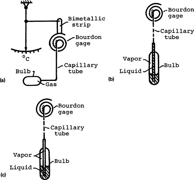
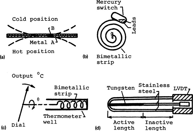
A bimetallic thermometer measures temperature by means of the differential thermal expansion of two metals. The bimetallic strip, shown in Fig. 9-1a, consists of a bonded composite of two metals. One of the metals is usually a copper alloy and the other Invar, a nickel steel with low thermal expansion coefficient. A temperature change will cause the bimetallic strip to bow, as shown in the figure.

Many types of bimetallic thermometers are commonly used. The bimetallic spiral with a mercury switch at its free end, shown in Fig. 9-1b, is for temperature sensing in a home thermostat. The bimetallic helix, shown in Fig. 9-1c, is placed in a thermometer well to serve as a mercury-in-glass thermometer. In this case, the output is the rotation of a pointer. The bimetallic probe, shown in Fig. 9-1d, can be placed in the duct of a jet engine to measure the average gas temperature [9]. Accuracy of bimetallic thermometers is from ±2 to ±5% and the upper temperature limit is about 500°F.

The familiar mercury-in-glass thermometer is an example of a filled thermometer that works on the expansion principle. It consists of a thin-walled glass chamber (bulb) filled with mercury, a uniform capillary in a glass stem with a scale, and an expansion chamber above the capillary for protection. The volume coefficient of expansion of mercury is about eight times that of glass. Due to the difference in coefficient between mercury and glass, the mercury rises up the capillary in the stem to indicate temperature. Other liquids are also used, because mercury freezes at −38.9°C.

FIGURE 9-1 Bimetallic thermometers (a) Bimetallic strip (b) Spiral (c) Helix (d) Differential.

If a thermometer is for partial immersion, an immersion ring is etched on the glass stem to indicate the correct depth of immersion. A total immersion type is preferred, because of the uncertainty of the exposed mercury thread to ambient temperature. When a total immersion thermometer is used in a partial immersion mode, the mercury thread above the liquid surface is not at the temperature of the bath. The temperature correction [10] is

$C_s=kn\left(T_B-T\right)$

(9-1)

where

 C_s = temperature correction

 k = correction factor (for mercury thermometers, k = 0.00016 for Celsius scale, and k = 0.00009 for Fahrenheit scale)

 n= number of degrees between the surface of the bath and the end of the mercury thread in the capillary T_B = indicated bulb temperature

 T_B = average temperature of the emergent mercury column, measured by means of another thermometer attached to the stem

Certified mercury-in-glass thermometers are widely used as working standards. For the total immersion type, the maximum accuracy is ±0.01°C from 0 to 150°C, and ±1°C from 300 to 500°C. Error due to viscous flow of glass under stress is about 0.2°F, due to hysteresis effect in heating and cooling is about 0.01 °F per 10°F, and due to external pressure is 0.2°F per atmosphere [11]. The ice point must be checked or the thermometer calibrated [12] if an accuracy of ±0.2°F or better is required.

The constant-volume gas thermometer, shown in Fig. 9-2a, is an example of a filled system that works on the pressure principle. It follows the gas law and has a pressure gage for its readout. The bimetallic strip shown in the figure is for ambient temperature compensation. The bulb of a gas-filled thermometer tends to be large, but the averaging effect of a large bulb may be advantageous for some applications.

FIGURE 9-2 Fluid-filled thermometers. (a) Constant-volume gas thermometer. (b) Bulb temperature > ambient temperature. (c) Bulb temperature < ambient temperature.

A vapor-pressure thermometer has a larger pressure change with temperature than that of a gas thermometer. The bulb can be smaller, and its operation is not influenced by dimensional changes of the bulb. The scheme shown in Fig. 9-2b is used when the bulb temperature is higher than the ambient temperature, and that in Fig. 9-2c used when the bulb temperature is lower than ambient. The discussion of these arrangements is left as an exercise.

Filled thermometers are used mostly for monitoring, although the pressure output can be utilized for pneumatic control. Their dynamic response is slow, and the time constant is of the order of 5 to 10 s. The trend is toward other types of sensors in order to obtain multipoint measurements, electric signal transmission, multiplexing, data logging, and computer control.

9-4.  THERMOCOUPLES

The thermocouple, or thermoelectric thermometer, is probably the most versatile and inexpensive temperature sensor. It is applicable for almost the entire temperature range, and is used for 50% of temperature measurements in industry [1]. Numerous metals, alloys, and even refractory materials can be paired as thermocouples [13]. Thermoelectric effects of materials, thermocouple “laws,” the gradient approach, construction, and practical thermocouple measurements are described in this section.

A.  Thermoelectric Effects

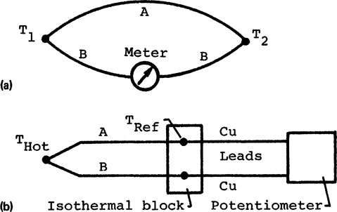
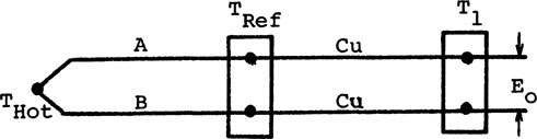
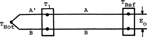
A thermocouple, shown in Fig. 9-3a, consists of two dissimilar metallic wires A and B. It measures the differential junction temperatures T₁ and T₂. The electric current or voltage measured by the meter in the circuit is a function of (T₁ – T₂). Generally, (1) the circuit is as shown in Fig. 9-3b, with the “hot” junction at T_Hot and the “cold” junction at T_Ref, the reference temperature of an electrically insulated isothermal block; and (2) the voltage is measured under zero-current condition by means of a thermocouple potentiometer (see Fig. 3-1b) or a sensitive high-input-impedance voltmeter. In other words, the thermal electromotove force (EMF) is measured with an open circuit.

There are three effects in a thermocouple circuit: the Seebeck, Peltier, and Thomson effects. The Seebeck effect describes the open-circuit voltage developed in a thermocouple circuit. The Peltier effect relates the reversible heating and cooling that usually occurs when an electric current crosses a junction between two dissimilar metals. The Thomson effect relates the reversible heating and cooling in a homogeneous conductor, subjected to a thermal gradient and a current flow. The physical effects can be explained from a macroscopic viewpoint by irreversible thermodynamics [14]. Generally, no current is drawn from a thermocouple circuit in a temperature measurement, and the Seebeck effect is sufficient to explain the circuit behavior.

FIGURE 9-3 Basic thermocouple circuits. (a) Thermocouple circuit. (b) Circuit with potentiometer readout.

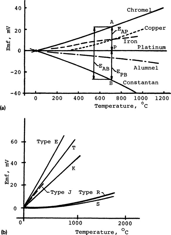
The voltage-temperature (E-T) characteristics of materials that are usually paired as thermocouples are shown in Fig. 9-4a. The slope S_A of the E-T curve of a material A is its voltage-temperature sensitivity, or the Seebeck coefficient, commonly called the thermoelectric power. S_A is a material property of A, but it can not be determined alone because it takes two dissimilar materials to produce a Seebeck EMF. Traditionally, pure platinum is used as the reference material. Hence S_A isnot an absolute coefficient. It should be written as S_AP = S_A – S_P, referring to platinum as the datum.

The Seebeck EMF E_AB from a pair of thermocouple wires A-B is illustrated in Fig. 9-4a. Let S_A be the sensitivity of material A (chromel). S_A is positive, because the E-T curve of A has a positive slope relative to platinum. The Seebeck EMF of material A is at a given temperature. Similarly, S_B is the sensitivity of material B (constantan). S_B is negative, and its Seebeck EMF is E_PB. Evidently, the Seebeck EMF of thermocouple A – B is E_AB = E_AP + E_PB. The Seebeck coefficient of thermocouple A–B is S_AB – S_PB.

If the thermal EMF of each material realtive to platinum is known, as shown in Fig. 9-4a, the EMF from the combination of two materials is the algebraic sum of their EMFs. In other words, it is only necessary to determine the voltage-temperature characteristics of each material with respect to a reference separately. Thermocouples can then be selected from pairs of these materials without a recalibration.

FIGURE 9-4 Voltage−temperature characteristics of thermoelements and thermocouples. (a) EMF of thermal elements versus platinum. (b) EMF of thermocouples.

A number of common thermocouples have been given designations by the Instrument Society of America ISA. Types E, J, K, and T are base-metal thermocouples. They are useful up to about 1000°C. Types S, R, and B are noble-metal thermocouples. They are useful up to about 2000°C.

Type E: chromel vs. copper-nickel alloy (constantan)

Type J: iron vs. copper-nickel alloy (constantan)

Type K: chromel vs. nickel-aluminum alloy (alumel)

Type T: copper vs. copper-nickel alloy (constantan)

Type S: platinum/10% rhodium vs. platinum

Type R: platinum/13% rhodium vs. platinum

Type B: platinum/30% rhodium vs. platinum/6% rhodium alloy

It is important to note that the names for the alloys above identify only the voltage-temperature characteristics of the alloys, but not the exact chemical composition. For example, the constantan for type J thermocouple is not thermoelectrically interchangeable with the constantan for type T.

Typical voltage-temperature characteristics of thermocouples are shown in Fig. 9-4b. Reference tables for thermocouples and the individual materials (thermoelements) relative to platinum are given in the NBS monograph 125 [15]. The Seebeck coefficients are also tabulated because they are not constants; that is, the Seebeck EMF is not linear with temperature. A scheme is used to designate the polarity of thermocouple wires. If wire A is positive relative to wire B, A is positive relative to B at the reference junction, when T_Hot > T_Ref (see Fig. 9-3b). The first-named material of a thermocouple is always positive, and the second-named material is negative. For example, iron is positive and constantan negative for an iron-constantan thermocouple. Color codes are used to identify the type of couples and the polarity of thermocouple wires; however, red, or red with a color trace, is always negative.

B.  Thermoelectric Laws

Referring to Fig. 9-5, the behavior of thermocouple of homogeneous materials can be described by thermoelectric laws [16].

1.  Intermediate Temperature

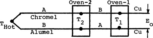
The thermal EMF E_AB of a thermocouple A−B due to temperatures T₁ and T₂ at the junctions is not affected by any intermediate temperature T₃ in the circuit, as shown in Fig. 9-5a. This allows thermocouple wires to be exposed to unknown and varying temperatures of the environment.

2.  Intermediate Metal

The thermal EMF E_AB of the circuit shown in Fig. 9-5b is not affected by any intermediate material C, provided that the junctions are at the same temperature, T₃. This permits the insertion of a material at any intermediate point in the circuit, such as shown in Fig. 9-5c. This becomes the basic thermocouple circuit shown in Fig. 9-3b, in which T₂ is at T_Ref of the isothermal block. Another implication is that soldering, welding, or other methods can be used to form thermocouple junctions, since the solder is an intermediate material. Thermocouple wires can be welded directly to a metal to measure its temperature, because the metal is an intermediate material. In fact, a weld may be unnecessary if good contacts can be made between the thermocouple wires and the metal.

3.  Successive Metals

From Fig. 9-5d, if the thermal EMF for thermocouple A-C of materials A and C is E_AC and that for C-B is E_CB, the EMF for the thermocouple A-B is E_AB = E_AC + E_CB. This allows the pairing of materials to form thermocouples.

4.  Successive Temperature

Referring to Fig. 9-5e, if E₂₁ is the thermal EMF due to the temperatures (T₂, T₁) and E₃₂ due to (T₃, T₂), the thermal EMF due to (T₃, T₁) is E₃₁ = E₃₂ + E₂₁. This permits the use of standard tables referenced at 0°C when the actual is at another temperature. For example, let T₃ = unknown temperature being measured, T₂ = 20°C = actual T_Ref, and T₁ = 0°C = standard reference temperature. From reference tables, E₂₁ = 1.019 mV. Let the measured thermal EMF be E₃₂ = 6.438 mV. Thus E₃₁ = E₃₂ + E₂₁ = 6.438 + 1.019 = 7.457 mV. The unknown T₃ from tables referenced at 0°C is 140°C.

C.  Gradient Approach to Thermocouple Circuitry

The gradient approach to thermocouple circuitry by Moffat [17] is an invaluable supplement to the thermocouple laws, which assume homogeneous materials. Yet inhomogeneity is often inevitable due to environmental contamination, cold work, and selective oxidation at high temperatures [18]. Note that a thermocouple always gives an output signal, regardless of its validity or the condition of the installation, unless a wire is broken. The gradient approach gives a systematic method of dealing with inhomogeneity, to troubleshoot, and to understand the behavior of more complex thermocouple circuits.

FIGURE 9-5 Circuits illustrating thermoelectric laws. (a) Homogeneous circuit. (b) (c) Intermediate metal. (d) Three metals. (e) Successive temperature.

The gradient approach states that the net thermal EMF E_net in a thermocouple, consisting of materials A and B, is due to the thermal gradient along the wires.

$E_{\text{net}}={\displaystyle {\int }_0^L{S}_A\frac{dT}{dx}dx+{\displaystyle {\int }_L^0{S}_B\frac{dT}{dx}dx}}$

(9-2)

where S_A and S_B are the total thermoelectric power of materials A and B, T = temperature, x = distance along the wires, and L = length of wire. It can be shown that Eq. 9-2 does not invalidate the thermoelectric effects described above. If S_A and S_B are not functions of position, then E_net is a function of the junction temperatures only.

$E_{\text{net}}={\displaystyle {\int }_{T_0}^{T_L}{S}_{A}dT+{\displaystyle {\int }_{T_L}^{T_0}{S}_{B}dT}}$

(9-3)

$E_{\text{net}}={\displaystyle {\int }_{T_0}^{T_L}\left(S_A-S_B\right)dT}$

(9-4)

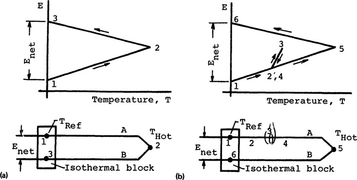
Let us illustrate the method with a simple example. The steps to find Enet for the thermocouple of materials A and B, shown in Fig. 9-6a, are as follows:

1.  Identify the points of interest (1,2,3) and assign nominal temperatures (T_Ref, T_Hot) to each point.

FIGURE 9-6 Gradient approach to find E_net. (a) E_net from thermocouple AB. (b) Intermediate temperature.

2.  Obtain the EMF versus temperature E-T calibration curves for the materials (see Fig. 9-4a).

3.  Starting from T_Ref at point 1, construct a curve in the E-T plot with the slope S_A of metal A until T_Hot at point 2, where A contacts B.

4.  Similarly, starting from point 2, construct a curve with the slope S_B back to T_Ref at point 3.

5.  The E_net for the thermocouple is from the E-T plot. Note that the graphical construction simply performs the line integration in Eq. 9-3.

Using the gradient approach, the E-T plot to verify the “law of intermediate temperature” is shown in Fig. 9-6b. The points of interest are from 1 to 6. Following the procedure above, the steps for obtaining E_net from the E-T plot are self-evident.

The decalibration of a thermocouple and the difficulties in its recalibration are well known. The thermocouple, shown in Fig. 9-7a, is used to measure the temperature of a metal bath. Since steep thermal gradients exist in the shaded section, this section will produce virtually the entire output EMF. Now, let the decalibration of the thermocouple wires, shown in Fig. 9-7b, occur in the sections between points 2-3 and 5-6, and the thermocouple is being recalibrated. The output E is from the recalibration with section 3-4-5 at the same temperature. The output E* is from the recalibration of the same thermocouple with section 2-3-4-5-6 at the same temperature, as shown in Fig. 9-7c. The EMF E* is generated by the unaffected wires, because all the affected wires are at a uniform temperature, that is, by the good thermocouple wires that have not been decalibrated. The result of the recalibrations is not predicted by the thermocouple laws above. The gradient approach is a useful operational method for troubleshooting.

D.  Reference Junctions

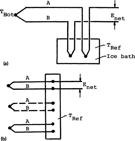
The thermal EMF E_net of a thermocouple is a function of (T_Hot – T_Ref). Hence the T_Ref of the reference junction must be known accurately. A ±1°C error in T_Ref will result in a ±1°C error in the measured temperature.

If the T_Ref is at 0°C, reference tables can be used to convert the measured EMF directly into temperature. An ice bath, shown schematically in Fig. 9-8a, is the simplest method to keep the T_Ref at 0°C. Details of an ice bath are described in the literature [19]. However, errors of more than ±1°C are often found in a poorly made ice bath [20]. An ice-bath is generally restricted to laboratory use, since it is awkward for a mobile test.

When the T_Ref is at a fixed temperature, software compensation can be used in a data acquisition system to convert the thermocouple output to temperature. For example, when the T_Ref is at 0°C, the conversion from the output x mV to T°C is expedited using a power series polynomial [21] such as

FIGURE 9-7 Recalibration of decalibrated thermocouple (a) Thermal gradient (b) Recalibration.

FIGURE 9-8 Thermocouple reference junctions. (a) T_Ref = 0°C. (b) T_Ref > 0°C.

$T=a_0+a_{1}x+a_2{x}^2+a_3{x}^3+\cdots +a_n{x}^n$

(9-5)

where the a’s are coefficients unique to each type of thermocouple. It is expedient to compute the temperature, because to store the lookup-table values in a computer could consume an inordinate amount of memory. Similarly, the temperature can be computed when the T_Ref is at a known elevated temperature instead of 0°C. A large isothermal block, as shownin Fig. 9-8b, can be used to maintain a fixed T_Ref for many themocouples.

Many schemes are used for hardware reference junction compensation [22]. Essentially, a compensating voltage E_Ref is added to the thermocouple output to simulate a constant T_Ref at 0°C. The scheme shown in Fig. 9-9a consists of a bridge circuit in which R₄ is temperature sensitive. Both R₄ and T_Ref are allowed to drift with the ambient temperature. The voltage change across R₄ is added to the thermocouple output for the compensation. The scheme shown in Fig. 9-9b is widely used in data acquisition systems. The T_Ref at the isothermal block is allowed to drift with the ambient temperature. A sensor at the isothermal block measures the T_Ref and actuates a circuit to yield a compensating voltage for the thermocouples.

FIGURE 9-9 Compensation for drifts in reference junction. (a) Bridge circuit. (b) Multiple input.

E.  Thermocouple Probes

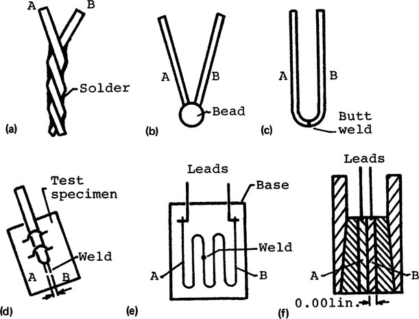
General- and special-purpose thermocouple probes are available for all temperature ranges [23]. General-purpose thermocouples are fabricated with a soldered, welded, or butt joint, as shown in Fig. 9-10a to c, in which A and B are thermocouple wires. Details for fabrication are given in the literature [24].

Three special-purpose thermocouples are illustrated in Figs. 9-10d to f. The intrinsic couple in Fig. 9-10d has an extremely fast response [25]. The couple is made from 0.001-in. wires, flattened to 200-μin. ribbons, and spot welded to the surface of a test specimen. The metal between the wires is an intermediate metal in the circuit. The time constant of this thermocouple is about 20 μs. The filament thermocouple shown in Fig. 9-10e is on an insulating base, similar to a strain gage. It can be attached to an irregular surface. The renewable junction thermocouple, shown in Fig. 9-10f is for extremely abrasive environments, such as the cone of a rocket engine. The sensor consists of 0.001-in. thermocouple ribbons insulated by 0.0002-in. mica. The abrasive action destroys the junctions of the thermocouple, but as fast as the old junctions are destroyed, new junctions are formed continuously by the abrasive action itself. In the same vein, a fine-wire platinum thermocouple (not shown) that destroys itself after one reading is available for temperature sensing of hot, molten metals with a 0. 25% accuracy (e.g., Leeds and Northrup, North Wales, Pennsylvania). The thermocouple is destroyed, but it has performed the task and costs less than a dollar.

FIGURE 9-10 Fabrication of general- and special-purpose thermocouple probes. (a) Soldered junction. (b) Beaded junction. (c) Butt-welded junction. (d) Intrinsic welded. (e) Filament sensor (courtesy of BLH Electronics, Waltham, Mass.). (f) Renewable junction (Model P, courtesy of Nanmac Corp., Indian Head, Md.).

Thermocouples for industrial applications are usually protected by sheathing, as shown in Fig. 9-11a to c, in which A and B are the thermocouple wires. The thermocouple may be insulated from the sheath, grounded to the sheath, or end welded to the sheath. For faster response, the thermocouple junction may protrude beyond the sheath (not shown).

Many special probes are commercially available. The probe shown in Fig. 9-11d is for sensing the surface temperature of a moving treadline of nylon or similar textile material [26]. The sensor consists of a cross arrangement with a thermocouple junction. Half of the cross is heated by an electric current, and the system is initially balanced. It is unbalanced when a treadline touches the junction. Temperature is measured by the current required to rebalance the system. Another example is a thermocouple in the form of a leave spring (not shown) to measure the temperature of a smooth-moving surface with velocity up to 300 ft/min (e.g., Series 68000, Omega Engineering, Inc., Stamford, Connecticut). The simple total-temperature probe shown in Fig. 9-11e consists of a thermocouple in a cavity. It is used when maximum economy, small size, and moderate accuracy are required.

FIGURE 9-11 Industrial general- and special-purpose thermocouple probes. (a) Insulated junction. (b) Grounded junction. (c) End-welded probe. (d) Filament probe. (e) Total temperature (from Ref. 27). (f) Pulse-cooled sensor (from Ref. 28).

The pulse-cooled probe shown in Fig. 9-11f extends the range of a chromel-alumel thermocouple (melting point 2550°F) to 7000°F. Normally, the thermocouple is air cooled. The solenoid valve shuts off the normal cooling air in order to measure the hot gas temperature T_gas. Thus a step temperature input is applied to the thermocouple, and it heats up as a first-order instrument (see Sec. 4-4C and Eq. 4-50):

$\text{τ}\frac{dT}{dt}+T=T_{\text{gas}}$

(9-6)

where τ is the time constant of the thermocouple, T the instantaneous temperature, and dT/dt the time rate of change of T. Both τ and dT/dt are measured with additional circuitry and a computer. Thus T_m can be estimated from the sum [τdT/dt + T]. The air is turned on again before the thermocouple becomes overheated.

F.  Practical Thermocouple Measurements

The overall error in a thermocouple measurement arises from many sources, from materials tolerances of wires, through all stages of the measurement, to data acquisition and noise documentation (see Secs. 3-7 and 3-8). Noise consideration is particularly important for thermocouple measurements, because of the low-level signal. For example, the Seebeck coefficient of base-metal thermocouples is of the order of 40 μV/°C and that of noble-metal couples 7 μV/°C. Hence the detection of 0.1°C requires resolutions of 4 μV and 0.7 μV, respectively, for the overall system. Instead of a systematic discussion of errors, some common problems in thermocouple measurements are described in this section.

1.  Thermocouple Wires

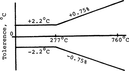
The quality of thermocouple wires must conform to standard reference tables. The industry-accepted ANSI Standard specify the allowable deviations for a temperature range [29]. The limits are materials tolerances for thermocouple wires only, that is, the possible error inherent of new thermocouples, prior to an exposure to adverse temperature or operating conditions. The error limit for special-grade wires is one-half that of the standard grade.

For example, the ASTM wire error [30] for a 8 AWG type J standard grade thermocouple is ±2.2°C from 0 to 277°C and ±0.75% from 277 to 760°C, as shown in Fig. 9-12. The possible error at 760°C is ±[2.2 + 0.0075(760 – 277)] = ±5.8°C, and the thermocouple still meets the guarantee. Again, this is an “acceptable” error for a new thermocouple, not necessarily its accuracy in service. Evidently, a thermocouple should be calibrated individually when a higher accuracy is required.

FIGURE 9-12 ASTM Standard for No. 8 AWG Iron–constantan thermocouple.

Less expensive extension wires for thermocouples have the same error limit, but their applications are restricted to lower temperature ranges. Extension-grade wires for base-metal thermocouples are of the same material as the thermocouples. Extension-grade wires for noble-metal thermocouples are made from less expensive proprietary alloys, to match the relative Seebeck coefficient of the thermocouples. Since extension wires are relegated to much lower temperature ranges, their thermal gradient is small and their contribution to the overall error is minimal.

2.  Practical Thermocouple Measurements

Some errors pertaining to thermocouple operations are described. Topics such as decalibration and reference junctions are not repeated here. Note that long-term stability and repeatability are often as important as absolute accuracy for some applications [31].

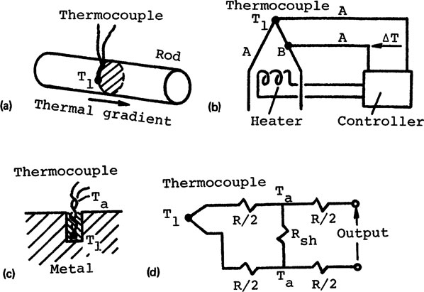
a. Thermal Shunting. A thermocouple is designed to measure the temperature of its “hot” junction. Thermal shunting is due mostly to the heat transfer at the hot junction. The thermocouple and its sheath may change the temperature of the hot junction and/or the local temperature at the point of measurement. In other words, thermal shunting is a thermal “loading” problem. Loading can occur under both steady-state and dynamic conditions.

A method to minimize thermal shunting in a surface temperature measurement is to place the leads from the hot junction along an isotherm, as shown in Fig. 9-13a. An elaborate system to avoid thermal shunting for a surface temperature measurement is shown in Fig. 9-13b.

FIGURE 9-13 3 Thermal and electrical shunting in thermocouples. (a), (b) Surface temperature measurement [(b) from Ref. 32]. (c), (d) Electrical shunts.

The thermocouple A–B is used to measure the surface temperature T₁ A portion of B is used as a differential thermocouple. A ΔT is detected if there is a thermal gradient along B, that is, if there is heat transfer to or from T₁. The signal ΔT isfed back to regulate a heater to render ΔT to zero. Thus the thermocouple wires are long an isotherm.

b. Electrical shunting. Electrical shunting may be due to a local short circuit or a deterioration of insulation. A short circuit is shown in Fig. 9-13c. The wires are shorted at T_a. Thus T_a become the temperature of the hot junction instead of T₁. A short between lead wires may be due to a mechanical damage. Moisture is often the culprit in lowering the resistance between leads. Moreover, the voltaic effect, due to moisture and the dye for wire insulation, or moisture and traces of flux from soldering, may be of the order of millivolts. The error follows no particular pattern [33].

The distributed shunt resistance in a thermocouple circuit is generally caused by a deterioration of insulation. The resistivity of common oxide insulations decreases exponentially with increasing temperature. Hence shunting is more prominent at high temperatures, such as in the insulation between the thermocouple wires in a sheath. It is a good practice to avoid using thermocouples near their maximum rated temperatures. The schematic of an electrical shunt is shown in Fig. 9-13d, where R_sh is the shunt resistance and R that of the thermocouple. Errors for different degree of shunting can be estimated [34]. Shunting can only degrade a temperature measurement. If R_sh ≪ R, the T_a at the shunt becomes a virtual junction in the circuit, and the measured temperature is dictated by T_a.

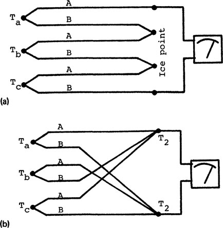
c. Series-parallel circuits. The series circuit (thermopile) shown in Fig. 9-14a is often used to increase the voltage output for greater sensitivity. All junctions must be electrically insulated from one another. A series circuit is analogous to batteries in series. The total voltage output is the sum of the individual voltages. If the hot junctions are at T_a, T_b, and T_c and the cold junctions at T_Ref, an arithmatic mean of the hot-junction temperatures can readily be obtained. This is the preferred method for temperature averaging.

The parallel circuit shown in Fig. 9-14b is also used for temperature averaging. The circuit is analogous to batteries in parallel, but current may flow among the thermocouples. The parallel circuit for averaging should be used with caution [35] since there is an undetermined current flow in the circuit and the voltage output is not entirely from Seebeck effect.

FIGURE 9-14 (a) Thermocouples in series. (b) Thermocouples in parallel.

3.  Data Transmission

Line-related noise, or error due to data transmission, is described briefly. The low-level dc signal from a thermocouple can be completely masked by noise pickups. A guard input [36] is generally provided at the digital voltmeter (DVM) for noise reduction.

A high common-mode voltage V_CM (see Sec. 3-1C) may occur in a thermocouple circuit. For example, assume that a grounded-junction thermocouple is used to measure the temperature of molten metal in an electric furnace. The thermocouple is placed in the molten metal and a 240 V_rms supply is used to heat the metal. Thus the V_CM at the thermocouple junction is on the order to 100 V.

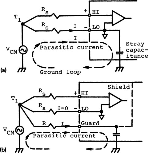
As shown in Fig. 9-15a, the V_CM causes a parasitic current I in the ground loop, which consists of the V_CM, the R_s of the LO lead, and the stray capacitance from the LO terminal of the DVM to ground. The IR_s drop in the LO lead is a signal between the HI and LO terminals at the DVM. This is interpreted as a signal from the thermocouple. Note that the HI terminal represents a higher input impedance than the LO terminal, because the power supply in the instrument is referenced to the LO terminal. Hence the ground loop flows through the LO lead.

FIGURE 9-15 Guard input in instruments to increase CMR. (a) Error due to parasitic current. (b) Passive guard.

The guard, shown in Fig. 9-15b, is physically a metal box surrounding the entire voltmeter circuit. It is connected to the shield of the thermocouple wires to shunt the parasitic current I. The guard input provides a low-impedance path for the V_CM. If R_s is 1 kΩ, guarding can yield a 40-dB common-mode rejection [37]. Many schemes, including active electronic components, are used to minimize line-related noise in instruments [38].

Other noise reduction techniques described in this book are filtering/shielding and analog-to-digital (A/D) conversion. The power-line-related noise and its harmonics are virtually eliminated when the integration dining the A/D conversion is an integer multiple of the power-line frequency (see Sec. 6-7E).

9-5.  RESISTANCE TEMPERATURE DETECTORS

Resistance temperature detectors (RTDs) are simply resistive elements. The resistance of metals increases with temperature. This common property is used for temperature sensing. Characteristics and applications of metallic RTDs are described in this section.

A.  Materials and Construction

Common materials for RTDs are platinum (from −260 to 1000°C), copper (from −200 to 260° C), nickel and Balco (70% Ni/30% Fe) (from −100 to 230°C), and tungsten (from -100 to 2500°C). The temperatures in parentheses are approximate figures. Temperatures recommended by manufacturers may differ considerably, depending on the construction of the sensor, materials for the capsule and sheathing, and the duty cycle in application. For example, a sensor can be exposed to a higher-than-steady-state temperature for a short duration without damage.

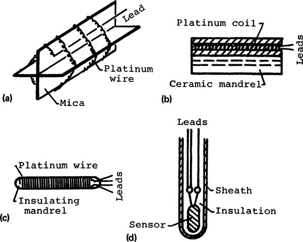
The sensing element can be broadly classified as wire-wound or film type. The latter is a more recent introduction. The wire-wound RTD, illustrated in Fig. 9-16a, is an early design to obtain strain-free wires. Helical coils of annealed platinum wire are loosely supported on a crossed mica web. The assembly is encapsulated in a glass tube for protection. This RTD is fragile and the thermal coupling between the sensing element and the point of measurement is poor.

The partially supported sensing element, shown in Fig. 9-16b, is more suitable for industrial applications. It consists of small coils of wire inserted into the axial holes of an insulating mandrel. Adhesive is introduced into the holes and the assembly is fired. Part of each turn of the coils is thus sintered to the mandrel, but the remainder of each turn is free.

FIGURE 9-16 Construction of RTD sensors and probe. (a) Platinum RTD. (b) Partially supported. (c) Fully supported. (d) RTD probe.

A fully supported and less expensive element is shown in Fig. 9-16c. The wire for sensing is wound on an insulating mandrel and then coated with an insulation. A fully supported element is more rugged and can survive shocks of 100g. It must be carefully designed to minimize a strain-related resistance change.

A RTD probe usually consists of an encapsulated sensing element in a protective sheath, as shown in Fig. 9-16d. General-purpose and special probes are commercially available [39]. Some are designed to operate in fluids, and others for the surface temperature measurement of solids. The time constant of wire-wound RTDs ranges from 0.5 to 10 s, depending on the heat transfer rate of the service condition.

Metallic film RTDs (not shown) are made by depositing a metal film on a substrate and then encapsulated. The film type is usually smaller than the wire-wound type and has a shorter time constant. Bondable film of nickel, Balco, or copper foil can be handled like strain gages (e.g., TG Series, Measurement Group, Inc., Raleigh, North Carolina). These RTDs are used for surface temperature measurements from -195 to 250°C. Due to the low thermal mass and large bonded area, the time lag of bondable RTDs is almost negligible.

B.  Characteristics and Standards

The resistance-temperature (R-T) characteristics of metals can be expressed as a polynomial:

$R=R_0\left(1+a_{1}T+a_2{T}^2+\cdots +a_n{T}^n\right)$

(9-7)

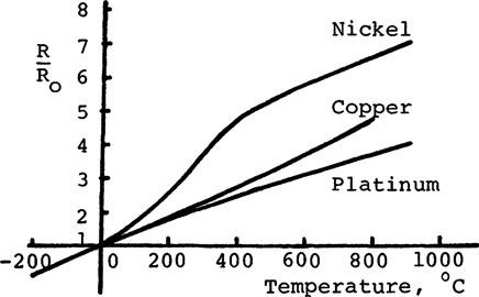
where the a’s are constants, R the resistance at a temperature T, and R₀ the resistance at base temperature T₀. A polynomial interpretation is used in the IPTS-68 to define temperatures from −190 to 660°C between fixed points by means of a platinum RTD [40]. Platinum and copper have almost linear E-T characteristics for a reasonable temperature range, as shown in Fig. 9-17. Nickel and Belco (70% Ni/30% Fe) are nonlinear, but Belco bondable sensors are easy to fabricate and the alloy has 2.4 times the resistivity of pure nickel. The result is lower-cost sensors and the ability to make higher-resistance sensors in smaller sizes [41].

When a material is almost linear over a temperature range, the first approximation from Eq. 9-7 can be used to determine temperature from a measured resistance.

$R=R_0\left(1+\text{α}T\right)$

(9-8)

FIGURE 9-17 Resistance-temperature characteristics of metals.

From Eq. 9-8, the a or average value of the temperature coefficient of resistance between 0 and 100° C is

$\text{α=}\frac{R\left({100}^{\circ }\text{C}\right)-R\left(0^{\circ }\text{C}\right)}{100\times R\left(0^{\circ }\text{C}\right)}$

(9-9)

where α has dimensions of (ΔR/R)/°C. Since a is a linearized value, the base temperature for the linearization, commonly at 0°C, must be specified [42] (see Fig. 2-11). An equivalent expression for Eq. 9-9 is the resistance ratio:

$\text{resistance}\text{ratio}=\frac{R\left({100}^{\circ }\text{C}\right)}{R\left(0^{\circ }\text{C}\right)}$

(9-10)

For example, if α = 0.003850 for a 100-Ω platinum RTD, R(100°C):R(0°C) = 138.50:100 = 1.3850:1.

Over a limited temperature range, an unknown temperature T can be calculated conveniently from the measured resistance R by means of Eq. 9-8.

$T=\frac{R/R_0-1}{\text{α}}$

(9-11)

For example, if R = 132.5Ω for a 100-Ω RTD and a = 0.00385, the temperature is T = (132.5/100 – 1)/0.00385 = 84.42°C.

Unfortunately, Eq. 9-11 must be used with caution, because there are several standards of a for platinum RTDs [43]. A manufacturer may use its own standard or that of several specifying agencies: for example, a = 0.00392 (US-MIL-T-24388) and α = 0.003850 (German-DIM43760). The difference between these two standards is 1.9%. Higher-purity platinum is required for the U.S.standard, but the trend is toward the Europen standard (DIM). Standards in some countries may differ. The British standard includes grade I and grade II. The nominal resistance of platinum RTDs at 0°C is 100Ω, but the American Scientific Apparatus Manufacturers Association standard is 98.129Ω [43].

The overall resistance of RTDs is not standardized. Platinum RTDs with resistances of 10, 50, 100, 200, 1000, and 2000Ω are available for different applications. Many “standard” values are found in sales literature, such as 10Ω for copper RTDs (T_Ref = 25°C), 120Ω for nickel RTDs (T_Ref = 0°C), and 670Ωfor nickel-iron RTDs (T_Ref = 25°C). The resistance ofthin film RTDs can be thousands of ohms.

C.  Circuits

Since a RTD is a resistive element, the basic circuit for its measurement is a bridge or an ohmmeter. A precision bridge is necessary for the resistance measurement. For example, the sensitivityof a 100-Ω platinum RTD is 0.385Ω, and a modest 0.1°C accuracy would require a resolution of 0.0385Ω. This is a small value, although a high-precision Mueller bridge with an uncertainty not exceeding 3 μΩ is possible [44]. On the other hand, a reasonable output is obtainable by measuring the voltage across an RTD. A current of 1 mA through a 100-ΩRTD gives an output of 100 mV, which is a large signal compared with that from a thermocouple. The associated I²R heating is examined later.

The null-balance bridge, shown in Fig. 9-18a, is a common technique for resistance measurements, where R is the resistance of the RTD and the DVM is used as a null detector (see Sec. 3-4). The circuit is modified, as shown in Fig. 9-18b, for three reasons.

1.  R must be physically separated from the bridge by extension wires to avoid subjecting the balancing resistors to the temperature of the RTD.

2.  The bridge has three lead wires. The source leads A and B have no effect on the bridge balance, and the third lead C is a sensing lead and carries no current.

3.  A potentiometer is used to balance the bridge. This avoids the uncertainty of the contact resistance for balancing at R₄, as shown in Fig. 9-18a.

When the bridge is used in an unbalanced mode, the voltage output V_o is not linear with the resistance in the RTD. This nonlinearity of an unbalanced bridge is acceptable for metallic strain gages, because ΔR/R is small in strain measurements (see Eq. 3-10), but the ΔR/R is large for a RTD. For example, if α = 0.00385, the ΔR/R for a ΔT = 100°C is 38.5%. If the bridge is initially balanced, the resistance R from Fig. 9-18a is

$R=\frac{V_{\text{ι}}+2V_o}{V_i-2V_o}{R}_2$

(9-12)

If the resistance R_L of the leads must be considered, the R of the RTD from the circuit in Fig. 9-18b is

$R=\frac{V_i+2V_o}{V_i-2V_o}{R}_2+\frac{4V_o}{V_i-2V_o}{R}_L$

(9-13)

The resistance R of a RTD can be measured with a constant-voltage or constant-current drive (see Sec. 3-5). The constant-voltage drive, shown in Fig. 9-18c, is not recommended, because the resistance R_L of the leads may cause a large error. For example, if R_L = 2Ω and the sensitivity of the RTD is 0.385 Ω/°C, the output is biased by an error of 2/0.385 = 5.2°C.

FIGURE 9-18 Basic circuits for resistance−temperature detectors. (a) Bridge circuit. (b) Bridge circuit with extended leads. (c) Constant-voltage drive. (d) Constant-current drive.

A four-wire ohmmeter circuit with a constant-current drive, shown in Fig. 9-18d (see also Fig. 3-51), is preferred, because the constant current is independent of the resistance of the source leads A and B. The input impedance of the DVM is of the order of 100 MΩ; therefore, the resistance in the signal leads C and D has no effect on the voltage signal at the DVM.

D.  Sources of Error

Both the thermocouple and the RTD are susceptible to errors from materials tolerances, electrical shunting, and thermal shunting. Materials tolerances for RTDs are similar to that for thermocouples (see Fig. 9-12). If the material standard is ±0.3°C at 0°C and up to ±3°C at 600°C, the readings from two RTDs at 600°C may differ by as much as 6°C. Thermal shunting may be more a problem with RTDs because the physical bulk of the RTD is greater than that of the thermocouple.

The RTD is also susceptible to errors in lead resistances, self-heating, and thermoelectric effects. The effect of lead resistance is minimized by using larger lead wires or a four-wire ohmmeter circuit as shown in Fig. 9-18d.

The self-heating effect is the I²R heating from a resistance measurement. It is stated as a self-heating error in °C/mW for a specific environment, such as in still air, air at 1 m/s, or water at 70°F and 3 ft/s. It is also called a dissipating constant, expressed in mW/°C. Self-heating is not problematic for most applications. For example, the I²R due to 1 mA through a 100-Ω RTD is 0.1 mW. If the self-heating error is 0.1°C/mW, the heating due to 1 mA is 0.01°C.

The measuring current I for a RTD ranges from 2 to 20 mA. A method to reduce self-heating and to increase sensitivity is to use short current pulses for the measurement. It takes several seconds to minutes for the self-heating to reach its final value. If the measuring current is in pulses of millisecond duration, the current can be increased by 10 to 100 times. Most pitfalls with platinum RTD applications result from using probes exceeding their specifications, particularly for temperatures greater than 550°C [45].

The thermoelectric effect is reduced by placing junctions of dissimilar metals closed to one another and by avoiding steep thermal gradients near these junctions. Alternatively, an ac can be used for the resistance measurement, since a thermal EMF is not detectable by ac instruments.

A mistake, peculiar to RTD measurements, is the inadvertent mixing of RTDs and readout or control devices [46]. As noted in Sec. 9-5B, the difference in a between the U.S. and DIM standard is 1.9%. A readout device for one RTD cannot be used for another RTD with a different specification.

9-6.  THERMISTORS

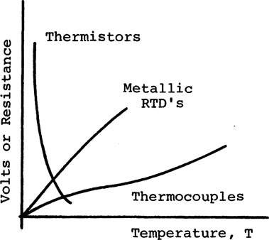
Both the RTD and the thermistor are simply resistive elements. Thermistors are used for temperature sensing as well as components in electronics and control systems [47]. The thermocouple, RTD, and thermistor as temperature sensors are compared briefly in this section.

The temperature ranges for the three type of thermometers are compared qualitatively in Fig. 9-19. The thermocouple has the widest temperature range but the lowest sensitivity. The RTD and thermistor do not require reference junctions. The RTD is more limited in temperature range but has higher sensitivity than the thermocouple. The advantages of RTDs are long-term stability and the capability for high precision. The thermistor has the least temperature range, typically from −100 to 150°C, but its sensitivity is 10 times that of the RTD. The resistivity of metals increases with temperature; therefore, RTDs have positive temperature coefficients. Thermistors are available with positive or negative coefficients. For temperature sensing, thermistors with negative resistance-temperature coefficients are used almost exclusively.

Thermistors are available commercially in the form of beads, rods, flakes, and so on. A thermistor probe can be made very small, and its time constant comparable with that of a thermocouple, but much shorter than that of a RTD. Within its narrow temperature range, the thermistor compares favorably with the RTD in stability, repeatability, and interchangeability, but is far superior in response time and sensitivity.

Figure 19 Characteristics of temperature transducers.

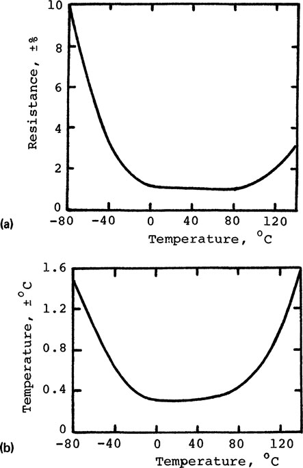
Materials tolerances for thermocouples, RTDs, and thermistors are specified in like manner. Tolerance data must be considered when speaking of errors or interchangeability. Thermistors with a 0.2°C interchangeability are available. Data for a typical thermistor are shown in Fig. 9-20. A tolerance is the possible error for a new probe, prior to exposure to service conditions, although the error represents the “worst case,” or limits, rather than typical error.

FIGURE 9-20 Characteristics of typical thermistor. (a) Resistance tolerance versus temperature. (b) Temperature tolerance versus temperature. (From Ref. 48.)

The negative resistance-temperature relationship of a thermistor can be expressed as [49]

$R=R_0{e}^{\text{β}\left(1/T-1/T_0\right)}$

(9-14)

where R is the resistance in ohms at the temperature T, T the absolute temperature K, R₀ the resistance at T₀, and 3000 < β < 5000 is a material constant. Generally, T₀ is at 980 K (25°C). The value of R₀ ranges from 100Ωto 1 MΩ, and a typical value is R₀ = 5 kΩ. The value of R for a thermistor may change from 3700 Ω at −80°C to 100Ω at 145°C.

The sensitivity S of a thermistor from Eq. 9-14 is

$S=\frac{d\left(R/R\right)}{dT}=\frac{-\text{β+}Td\text{β}/dT}{T^2}$

(9-15)

$S=\frac{d\left(R/R\right)}{dT}\simeq -\frac{\text{β}}{T^2}$

(9-16)

$\frac{dR}{dT}\simeq -\frac{\text{β}}{T^2}R$

(9-17)

From Eq. 9-16, if β = 4000, T = T₀ = 298 K, and R₀ = 5 kΩ, the sensitivity is 0.045, or ΔR/R = 4.5% per °C. For a platinum RTD, if the sensitivity from Eq. 9-8 is 0.00385, the ΔR/R is 0.38% per °C. Hence the thermistor has 10 times the sensitivity of a RTD.

An empirical expression is used to convert the measured resistance R of a thermistor into temperature T [48].

$\frac{1}{T}=A+B\text{ln }R+C{\left(\ln R\right)}^3$

(9-18)

where R is in ohms, T in kelvin, and A, B, and C are curve-fitting constants. Their values are obtained by substituting three pairs of values of (R,T) about the operating range into Eq. 9-18 to obtain three simultaneous equations. The equations are then solved simultaneously to give the constants. The output of a thermistor is nonlinear, but the computation of T from a measured value R is not a problem in data acquisition.

Due to the high resistance and high sensitivity, the effects of lead-wire resistance and self-heating are negligible for thermistors. For example, if R₀ = 5 kΩ and ΔR/R = 4.5% per °C, the resistance change is ΔR = 225 Ω/°C. This is much larger than the resistance of 500 ft of No. 18 AWG copper extension wire (6.5 Ω/1000 ft). The self-heating effect is also small. If R₀ = 5 kΩ and the rated dissipation constant is 4 mW/°C, an I²R input of 0.04 mW relates only to 0.01°C of self-heating, but gives an output of 0. 45 V.

All the circuits in Fig. 9-18 can be used for thermistors, because of neglectable lead-wire and self-heating errors. Using the bridge in Fig. 9-18a in an unbalanced mode with equal resistors and initial V₀ = 0, the measured resistance R is

$R=R_0\frac{1+2V_0/V_i}{1-2V_0/V_i}$

(9-19)

The resistance R can be used to calculate the temperature T from Eq. 9-18, or to obtain T from tables. For the four-wire ohmmeter circuit in Fig. 9-18d, the current I is constant and R at the measured temperature T is

$R=R_0\frac{V}{V_0}$

(9-20)

where R₀ and V₀ are the respective initial values at T₀, and R and V are the respective values at the temperature T.

9-7.  PYROMETERS: PRINCIPLES [50]

A pyrometer, or radiation thermometer, is a noncontact instrument that measures the electromagnetic radiation emitted from a body and infers its temperature from the detected radiation. All objects emit radiation by virtue of their temperature. Principles employed for pyrometry are Planck’s law and the Stefan-Boltzmann law. It will be shown in Sec. 9-8 that pyrometers can generally be classified as narrowband and broadband. Planck’s law is used for the narrowband and the Stefan-Boltzmann law for the broadband or total radiation pyrometer.

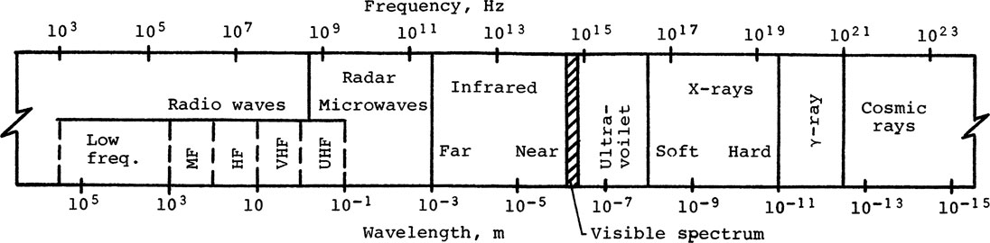
Pyrometers are applicable for wide temperature ranges and are not restricted to high temperatures. The electromagnetic radiation spectrum is shown in Fig. 9-21. A portion of the spectrum can be used for pyrometry, and the spectrum normally used is from 0.3 to 40 μm. The visible spectrum, shown crosshatched, occupies only a very limited band, from 0.35 μm (blue-violet) to 0.78 μm (red). In the visible spectrum, a piece of steel in a furnace appears red at about 600°C, and it changes from a dull red, through orange and yellow, to white at about 1600° C. The infrared spectrum is not visible, but infrared pyrometers are common. A commercial unit can be used to −100°C (e.g., Model ST, Barber-Colman, Loves Park, Illinois). The frequency of radiation for other applications is also shown in the figure. As radiation propogates at the speed of light at 3 × 10⁸ m/s, the product of frequency and wavelength is 3 × 10⁸ m/s.

A.  Physical Laws

The distribution of radiant power intensity from a blackbody at a given temperature for varying wavelengths is described by Planck’s law in Eq. 9-21. The concept of a blackbody will be described presently.

FIGURE 9-21 Electromagnetic radiation spectrum.

$W_b\left(\text{λ,}T\right)=\frac{2\text{π}{c}^{2}h}{{\text{λ}}^5\left[e^{\left(hc/k\text{λ}T\right)}-1\right]}=\frac{C_1}{{\text{λ}}^5\left[e^{\left(C_2/\text{λ}T\right)}-1\right]}$

(9-21)

where

W_b(λ, T) = radiant power intensity from a blackbody in W/m³

λ = wavelength in m

T = absolute temperature in kelvin

h = Planck’s constant = 6.625 × 10^–34 J.s

c = speed of light = 3 × 10⁸ m/s

k = Boltzmann’s constant = 1.380 × 10⁻²³ J/K

C₁ = 2πc²h = 3.74 × 10⁻¹⁶ W·m²

C₂ = hc/k = 1.44 × 10⁻² m·K

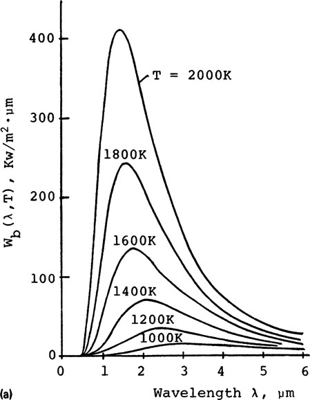
The distribution of W_b (λ, T) versus λ is shown in Fig. 9-22a. W_b(λ, T) is the intensity of radiant energy emitted from a blackbody at temperature T and wavelength λ, per unit time, per unit wavelength interval, per unit area, per unit solid angle, that is, the radiation from a flat surface onto a hemisphere. It is also called the hemispherical spectral radiant intensity.

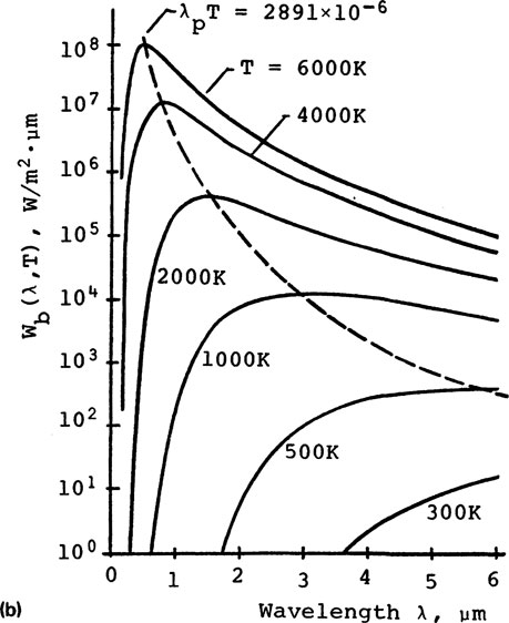
FIGURE 9-22 Blackbody radiation power intensity W_b(λ, T)

Wien’s radiation law is often used instead of Planck’s law:

$W_b\left(\text{λ,}T\right)=\frac{C_1}{{\text{λ}}^5{e}^{\left(C_2/\text{λ}T\right)}}$

(9-22)

The difference between the two equations is the −1 term in the demominator. The −1 can be omitted when the exponential term is large compared with unity. For example, for T = 2500 K and λ = 1 ¼m, values of W_b(λ, T) from the two equations differ only by 0.3%. It may be of interest to note that historically Wien’s law preceded Planck’s law. The wavelengths λ_p at peak intensities for higher temperatures skew toward shorter wavelengths, as shown in Fig. 9-22b. This is described by Wien’s displacement law:

${\text{λ}}_{p}T=2891\times {10}^{-6}$

(9-23)

The area under each of the curves in Fig. 9-22 is the total power W_b(T) emitting from a blackbody at a given temperature T. This is described by the Stefan-Boltzmann law in Eq. 9-25.

$W_b\left(T\right)={\displaystyle {\int }_{\text{λ}}{W}_b\left(\text{λ},T\right)d\text{λ}}$

(9-24)

$W_b\left(T\right)=\sigma T^4$

(9-25)

where σ = 5.67 × 10^–8 W/m²·K is the Stefan-Boltzmann constant. The total power emitting from a blackbody is proportional to the fourth power of its absolute temperature.

B.  Emittance

The concepts of blackbody and emittance are central to the study of pyrometry. Let us first describe a blackbody. Imagine that radiation is beamed at a small hole on the surface of a hollow sphere. All the energy entered the hole is being absorbed because there is no escape. Hence the area of the hole receiving the radiation is a perfect absorbing surface, or blackbody. Black here refers to the ability to absorb radiant energy rather than color.

Conversely, radiation emitting from the hole on the surface of the hollow sphere is also radiation from a blackbody. From KirchhofPs law, the absorptivity of a material is equal to its emissivity, and a perfect absorber is also a perfect emitter. The emittance of a blackbody is unity; that is, a blackbody would emit the maximum amount of thermal radiation possible for a given temperature. If the sphere is at a constant temperature, radiation emitting from the hole is radiation from a blackbody, as described by Planck’s law in Eq. 9-21. In practice, the blackbody behavior can be approximated by means of a blackened conical cavity of about 15° at a constant temperature. A blackbody is useful for the calibration of pyrometers and as a thermal reference in instruments.

Emittance describes the relative amount of thermal energy radiating from a body. It is expressed as a ratio of the actual radiation W_a versus the blackbody radiation W_b at the same temperature. The emittance of an actual body is always less than unity, and W_a < W_b. From Eq. 9-21, the spectral emittance ε_λ. of a body at a constant temperature T is defined as

${\text{ε}}_{\text{λ}}=\frac{W_a\left(\text{λ},T_m\right)}{W_b\left(\text{λ},T\right)}\le 1$

(9-26)

where T is the target temperature, or the true temperature, and T_m is the measured temperature. In other words, if the target were a blackbody, the pyrometer would give the true temperature T. Since W_a(λ, T_m) < W_b(λ, T), the measured temperature is T_m. Evidently, ε_λ ≤ 1 and T_m < T, because the greater the amount of energy emitting from the target, the higher the temperature indicated by a pyrometer. The integration of Eq. 9-26 gives the total emittance ε due to all wavelengths:

$\text{ε}=\frac{W_a\left(T_m\right)}{W_b\left(T\right)}\le 1$

(9-27)

A gray body is a body whose emittance is independent of wavelength; that is, ε_λ = constant for all λ at a given T, or ε_λ = ε. Hence the actual W_a(λ, T_m) versus X curve has exactly the same shape as that for W_b(λ, T) shown in Fig. 9-22.

Emittance rather than emissivity is used in this discussion. Like emittance, emissivity is a ratio, but emissivity is a material property in the sensethat it is defined only for highly polished surfaces or controlled conditions [51]. Emittance describes an actual condition. It depends on many variables, such as size and shape of an object, surface roughness and oxidation, angle of viewing, temperature, wavelength, and so on. There is no simple relationship between the variables [52].

It will be shown in the next section that the importance of using accurate values of emittance in pyrometry cannot be overstated.

1.  Due to the difference in emittance, two targets at the same temperature may emit significantly different amount of energies. Consequently, the same pyrometer may give different readings for two bodies of identical temperature.

2.  Due to a change in emittance, such as oxidation or even angle of viewing, the same pyrometer may give different readings for the same body at the same temperature.

C.  Measurement Uncertainty

The emittance of an object must be known in a temperature measurement. An inherent error in pyrometry is due to the uncertainty in the value of emittance. The error relating to Planck’s law and the Stefan−Boltzmann law is described in this section.

Consider a narrowband pyrometer employing Planck’s law for a temperature measurement at a known wavelength λ From Eq. 9-26, T_m relates to theactual radiation W_a(λ, T_m) from the target, but the target temperature T relates to W_b(λ, T). Writing W_b(λ, T) explicitly and substituting into Eq. 9-26, we get

$W_a\left(\text{λ},T_m\right)=\frac{{\text{ε}}_{\text{λ}}{C}_1}{{\text{λ}}^5\left[e^{\left(C_2/\text{λ}T\right)}-1\right]}$

(9-28)

Although W_a(λ, T_m) is known, there are two unknowns in one equation in Eq. 9-28, ε_λ and T. The procedure in using a pyrometer is to assume a reasonable value for the emittance ε_λ, adjust the pyrometer accordingly, and then proceed with the measurement to deduce the temperature T.

The error in temperature due to the uncertainty in emittance ε_λ can be estimated from Eq. 9-26. Using Wein’s law to simplify the calculation, defining

$\begin{array}{lll}{W}_a\left(\text{λ,}{T}_m\right)=\frac{C_1}{{\lambda }^5{e}^{\left(C_2/\text{λ}{T}_m\right)}}\hfill & \text{and}\hfill & W_b\left(\text{λ},T\right)=\frac{C_1}{{\text{λ}}^5{e}^{\left(C_2/\text{λ}T\right)}}\hfill \end{array}$

(9-29)

substituting Eq. 9-29 into Eq. 9-26, and simplifying, we obtain

$T=\frac{T_m}{1+\left(\text{λ}{T}_m/C_2\right)\left(\ln {\text{ε}}_{\text{λ}}\right)}$

(9-30)

where T is the true temperature of the emitting body, T_m the measured temperature, and ε_λ. the assumed emittance. The error dT/T from Eq. 9-3 is

$\frac{dT}{T}=\frac{\text{λ}T}{C_2}\frac{d{\text{ε}}_{\text{λ}}}{{\text{ε}}_{\text{λ}}}$

(9-31)

The error in T is not greatly influenced by the uncertainty in ε_λ for this type of pyrometer. For example, if λ = 0.65 μm and T −2000 K, a 10% error in ε_λ results only in a 0.90% error in T.

Consider a broadband pyrometer using the Stefan-Boltzmann law for a temperature measurement. Substituting Eq. 9-25 into Eq. 9-27 and simplifying, we get

$T=T_m{\text{ε}}^{-1/4}$

(9-32)

$\frac{dT}{T}=-\frac{1}{4}\frac{d\text{ε}}{\text{ε}}$

(9-33)

where T is the true target temperature, T_m the measured temperature, and E the total emittance. The uncertainty due to the value of emittance is greater for this instrument than that using Planck’s law above. For example, a 10% error in ε results in a 2.5% error in T.

It should be restated that the uncertainty due to the value of emittance is inherent in pyrometry. Emittance, however, is a complex relation of many variables and not a simple constant. No single emittance value can be used for all types of pyrometers, for widely different temperatures, or for the same pyrometer under different conditions. For example, the spectral emittance ε_λ of tungsten increases with increasing temperature and decreasing wavelength, but existing theory is insufficient to predict this behavior accurately [52].

Finally, the calibration for emittance uncertainty depends largely on past experience.

1.  It is proper to use relaible published data when similar conditions exist. The error can then be estimated from Eq. 9-31 or 9-33.

2.  It may be possible to create a blackbody condition at the target.

3.  Preliminary tests can be performed to obtain typical emittance values for various target conditions. For example, pyrometer readings can be made for targets of known temperatures, obtained by means of contact thermometers such as thermocouples. This is creating one’s own lookup table.

4.  The effect of emittance may be minimized by using a ratio pyrometer. This is discussed in the next section.

9-8.  PYROMETERS

The theory of pyrometry described above is not new. In response to current demands [53], however, design efforts have led to more convenience, improved sensitivity, new materials, faster response, specialized applications, and (unfortunately) greater variations in detail. In this section we describe applications, general construction of narrowband and broadband pyrometers, and components common to the instrument.

Pyrometers are noncontact radiation instruments for measuring the average temperature of objects. The noncontact, radiation, and averaging features are necessary for some problems. These features also dictate the areas of application.

A noncontacting instrument is used when a contacting type, such as a thermocouple, is not practical. For example, pyrometers are used for temperature measurements of (1) delicate surfaces, such as paper and plastic sheets; (2) fast-moving objects, such as ingots in a steel mill; and (3) onetime applications, such as determining the temperature of high-tension power lines and energy audit of buildings [54]. Furthermore, a thermocouple must assume the high temperature of the object, but the sensor of a pyrometer is at a low temperature.

Temperature measurement by radiation is a convenience under hostile environmental conditions, such as in the presence of strong chemicals, high pressures, and extreme temperatures. The temperature of an object under strong electrical interference, as in an induction heating furnace, can be measured routinely by means of pyrometers. Fiber optics can be used for the signal transmission of high temperatures, such as inside the catalytic converter of an automobile (e.g., Model TM-2, Vanzetti Systems, Stoughton, Massachusetts). It would be difficult to measure the temperature of an erupting volcano by any other means.

The averaging effect has many advantages for some problems, such as averaging the surface temperature of a wall or that of an ocean [55]. The target size can be very large or extremely small. For example, an infrared microscope is capable of focusing on an area with a diameter as small as 0.0003 in. (e.g., Barnes Engineering Co., Stamford, Connecticut). For most applications, the target size of infrared pyrometers ranges from 0.10 in. at 2 in. to 2 in. at 10 in. (e.g., Omega Engineering, Inc., Stamford, Connecticut).

To satisfy diverse requirements, pyrometers are available with numerous features. Tables of instruments, specifications, and manufacturers are published periodically in trade journals [53] and buyer’s guides. Some manufacturers have a “complete” line of products, for applications from aircraft engines to health care [56], Recent advances are largely associated with infrared and spectral-selective devices, that is, pyrometers to operate in a selected spectrum, optimized for a given task.

A.  Brightness Pyrometers

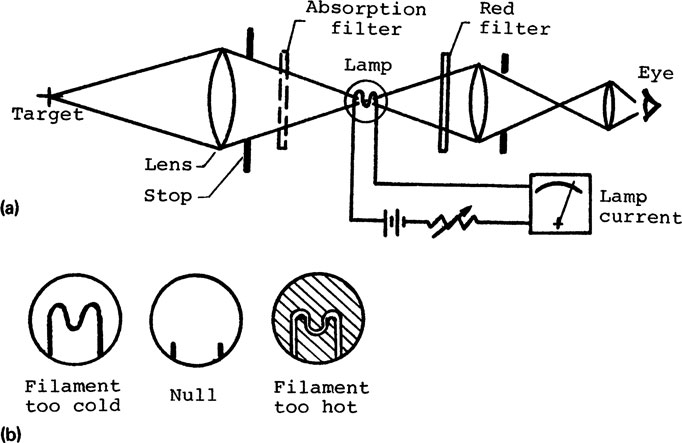
The brightness pyrometer, also known as the disappearing filament or optical pyrometer, is the most accurate instrument for high-temperature measurements above 700°C. It is employed to realize the IPTS-68 above the gold point at 1063°C. A classical form of the instrument consists of the optics, an absorption filter, a tungsten lamp of variable brightness, a red filter, and an eyepiece, as shown in Fig. 9-23a. The absorption filter is for viewing targets above 1300°C.

The pyrometer operates with an extremely narrow band. The red filter has a sharp cutoff at λ < 0.63μm. The human eye provides the cutoff at the longer wavelengths of the visible spectrum. Thus the effective wavelength of the instrument is 0.653 μm. The test object and the lamp filament are viewed simultaneously. Hence the brightness of the target and that of the lamp filament are compared under monochromatic conditions.

The brightness of the lamp filament is adjusted manually until the filament seems to disappear, as shown in Fig. 9-23b, that is, when the test object and the filament are at the same temperature. The unknown target temperature is T and that of the lamp filament is T_m in Eq. 9-30. The spectral emissivities of target materials at 0.65 μm are given in the literature [51]. It will be shown that the manual adjustment can be automated.

The ratio or two-color pyrometer is an attempt to minimize the emittance uncertainty in pyrometry. The instrument is essentially a combination of two optical pyrometers, using two separate filters in order to operate at two separate wavelengths λ₁ and λ₂. The actual radiation received at λ₁ is W_a(λ₁, T_m1), as shown in Eq. 9-26, and that at λ₂ is W_a(λ₂, T_m2). The ratio R of the radiations at λ₁ and λ₂ is

FIGURE 9-23 Schematic of a brightness (optical) pyrometer (a) Brightness (optical) pyrometer (courtesy of Leeds and Northrup Co., North Wales, Pa.) (b) Disappearing filament.

$R=\frac{{\text{ε}}_{\text{λ}1}}{{\text{ε}}_{\text{λ2}}}\frac{{\text{λ}}_2^5}{{\text{λ}}_1^5}\frac{e^{\left(C_2/{\text{λ}}_{2}T\right)}-1}{e^{\left(C_2/{\text{λ}}_{1}T\right)}-1}$

(9-34)

where R is a known measured value. The ratio pyrometer is free of emittance error if ε_λ1 = ε_λ2, since the true temperature T of the target can be calculated directly from Eq. 9-34.

If the values of ε_λ1 and ε_λ2 are unequal, the target temperature can be estimated by two methods. (1) The error is negligible if a narrow spectrum is chosen such that ελ varies slowly with X, that is, if the ratio ε_λ1/ε_λ2 is approximately unity. (2) The ratio is assumed unity to obtain an approximation. Then the value of the ratio is estimated to provide a correction. First, if exp(C₂/λT) ≫ 1 and the ratio ε_λ1/ε_λ2 is assumed to be unity, the approximated temperature T_R from Eq. 9-34 is

$T_R=\frac{C_2\left(1/{\text{λ}}_2-1/{\text{λ}}_1\right)}{\ln \left[R{\left({\text{λ}}_1/{\text{λ}}_2\right)}^5\right]}$

(9-35)

Now, the ratio of the unequal emittances ε_λ1/ε_λ2 is estimated. Substituting Eq. 9-35 into Eq. 9-34 and simplifying, the estimated temperature T is

$T=\frac{T_R}{1+\left[{\text{λ}}_2{\text{λ}}_1/\left({\text{λ}}_2-{\text{λ}}_1\right)\right]\left(T_R/C_2\right)\ln \left({\text{ε}}_{\text{λ1}}/{\text{ε}}_{\text{λ2}}\right)}$

(9-36)

B.  Wideband and Selected-Band Pyrometers [57]

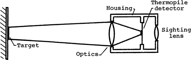
The wideband or total-radiation pyrometer operates on the Stefan−Boltzman law. The instrument consists of the optics, a detector, the housing, and sighting lenses, as shown in Fig. 9-24. The optics concentrate the radiation from a target onto a small detector. Thermal or photon detectors are used. The housing may be thermostatically control for greater thermal stability.

A thermal detector senses the radiation and infers the target temperature from its own temperature. Thermistors and RTDs are thermal detectors and are called bolometers. Since a thermal detector depends on its own temperature to infer the detected radiation, its time constant is fairly long, from 5 ms to 0.5 s. A pyrometer with a thermal detector is essentially a first-order instrument. A simplified analysis of the pyrometer shown in the figure with a thermopile detector gives

$C\left(T_1-T_2\right)=\text{ε}\sigma T^4$

(9-37)

where T is the target temperature, T_1,2 are those of the thermopile, C is a constnat, σ the Stefan−Boltzmann constant, and ε the total emittance of the target. Another type of thermal detector is pyroelectrics. These have high response speeds, because the electrical output depends on the timerate of change in temperature rather than on the detector temperature itself.

A photon detector generates a voltage as a function of its detected photon flux. The flux frees electrons in the detector to produce a measurable electrical output. As the reaction occurs at an atomic level, photon detectors have very high response speeds. In fact, photon detectors can be used for infrared scanning, that is, to display the dynamic temperature distribution of a small target on a TV monitor. The spectral response of photon detectors is not constant compared with that of thermal detectors, its output voltage also varies approximately as T³, instead of to the fourth power as in the Stefan-Boltzmann law.

FIGURE 9-24 Schematic of a total radiation pyrometer.

The disadvantage of a truly wideband pyrometer is the uncertainty in the value of emittance. The spectral emittance of most materials is not constant over the entire bandwidth; therefore, the total emittance is also temperature dependent. Most pyrometers include an emittance adjustment, from 0.2 to 1.0.

The study of pyrometry is further complicated by the fact that radiant energy can be partially absorbed, reflected, and transmitted. This is expressed as

$\text{ε}=1-r-t$

(9-38)

where ε is the emittance, r the reflectance, and t the transmittance. The transmittance of a solid body is t = 0. The values of ε, r, and t are not constants. For example, soda-lime glass is transparent to solar radiation but opaque to infrared; that is, a material can be opaque or transparent, depending on the wavelength.

Recent advances have been largely associated with spectrally selective or narrowband pyrometers in the infrared spectrum. A selected-band pyrometer dictates the spectrum with which to operate. It may be designed (1) to match or to optimize the spectral properties of its components, or (2) to select the most advantageous spectrum for the task. For example, in mapping the temperature of the earth’s surface from space, the main barriers are CO₂ and water vapor in the atmosphere. The mapping can be performed by using the 8- to 13μm “window” in the infrared spectrum, because CO₂ and water vapor are largely transparent for this spectrum and for the temperature range considered. The other side of the coin is that filters can be used to pass the15-μm band for which CO₂ is a strong emitter. Thus air temperatures miles ahead of an aircraft can be measured.

C.  Components

Some components common to pyrometers are described in this section [58]. The basic items are the optics, filters, detectors, optical choppers, and black bodies for thermal reference. Electronics are omitted in this discussion. The sighting path between the target and the pyrometer is also an integral part of the measuring system, since the radiation may be partially absorbed, reflected, or transmitted in the transmission path, as shown in Eq. 9-38.

The sighting path must be transparent to the radiation. Any interference due to dust, flame, fumes, moisture, or background radiation is noise in the signal to the pyrometer. A purging tube with clean nonabsorbing gas is used when the interference cannot be filtered out optically. The gas, or the medium for the signal transmission, need only be transparent for the operating spectrum of the pyrometer. For example, fiber optics can be used instead of a purging tube for signal transmission at high temperatures.

Optics, filters, and detectors for pyrometers have different spectral sensitivities. In other words, the sensitivity versus wavelength plot of a material may peak sharply, or remain fairly flat with cutoffs at both ends of a given spectrum, like the frequency response characteristics of an instrument (see Fig. 4-22). The characteristics of the components should be optimized in order to work as an integral unit for the intended application. It is difficult to give details on spectral sensitivity of materials. For example, glass is opaque for wavelengths greater than 2.5 μm. Hence glass lenses are not suitable for most infrared detectors, but glass can be used for a lead sulfide detector, which has a spectral sensitivity peak at 2 μm. Furthermore, light of different wavelengths is focused differently; the result is poor targetdefinition or background noise unless the optical system is achromatic, such as focusing mirrors or compound lenses. Visible and infrared radiation follow the same optical laws, but some infrared lenses, such as arsenic trisulfide, are opaque to the visible spectrum.

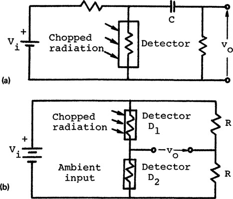
An optical chopper (see Fig. 3-54) can be used (1) to convert the dc input to a detector to ac, (2) to allow radiation of different wavelengths to reach the detector alternately, or (3) to compare the radiation from a target with that of a reference. For a dc-to-ac conversion, the chopper simply interrupts the radiation from the target to the detector. A circuit with chopped radiation to a thermistor detector is shown in Fig. 9-25a. This is the ballast circuit for strain gages (see Probs. 1-3 to 1-5). The ac output can then amplified with an ac amplifier. This circuit is less susceptible to the slowly varying ambient temperature. Another scheme uses two detectors in a bridge circuit, as shown in Fig. 9-25b (see Fig. 3-33). The detector D₁ is exposed to the chopped radiation, but D₂ is shielded from radiation and it is at the controlled temperature of the housing.

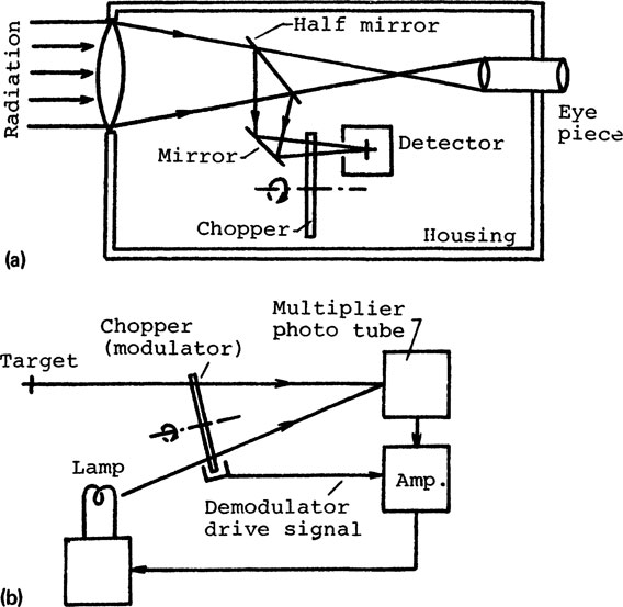
The pyrometer with an optical chopper, shown in Fig. 9-26a, is suitable for comparing the radiation from a target with that of an internal black-body [59]. If the optical chopper has a mirror-finished surface, radiation from a built-in blackbody (not shown) can be reflected to the detector.

FIGURE 9-25 Circuits for chopped radiation detection. (a) Ballasat circuit. (b) Bridge circuit.

Thus the detector receives radiation from the target and a blackbody alternately. If an internal blackbody is not used and the chopper has a blackened surface, the detector receives radiation alternately from the target and the chopper alternately. Thus the controlled temperature of the housing becomes the thermal datum. The beam splitter simply allows direct sighting of the target.

The output from the detector is a train of square pulses. Its amplitude relates to the difference in radiation received between the target and the blackbody. This is an amplitude-modulation process (see Sec. 5-4A). The chopper modulates the input to the detector. A magnetic pickup can be placed at the chopper to obtain a synchronous signal for the phase-sensitive demodulation (see Figs. 5-10, 12). The output is an analog signal corresponding to the temperature detected by the target. If the chopping frequency is 180 Hz, the time constant of the system is about 8 ms. Alternatively, the temperature of the blackbody can be adjusted by means of feedback for the system to operate in a null-balance mode (e.g., Barnes Engineering Co., Stamford, Connecticut), but the higher accuracy is obtained at the expense of speed of response(see Sec. 3-2).

Similarly, the automatic optical pyrometer, shown in Fig. 9-26b, employs an optical chopper to modulate the radiation from the target and the standard lamp to the photomultiplier tube. The chopper is at a fixed frequency. The standard lamp is used as an internal thermal reference instead of a blackbody. To operate in the null-balance mode, the brightness of the lamp is adjusted by means feedback until a null intensity is sensed by the photomultiplier. To operate in the unbalanced mode, the brightness of the lamp is unchanged, and the difference in brightness gives the output.

FIGURE 9-26 Pyrometers with optical chopper. (a) Optical head with internal reference. (b) Automatic brightness pyrometer (Model 8641 Mark 1, courtesy of Leeds and Northrup Co., North Wales, Pa.).

9-9.  MISCELLANEOUS TEMPERATURE SENSORS

Several temperature sensors for industrial applications are described briefly in this section. Many new sensors, such as the Johnson noise thermometer [60], are made possible by advances in electronics in recent years, but they are used mostly in the laboratory.

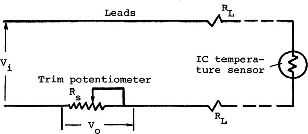
The integrated-circuit (IC) thermometer is a semiconductor-based temperature sensor, developed in the electronic industry. It is widely accepted and has a market share of about 5%. Only an unregulated power supply is required for the IC. The sensor has good linearity and an analog output of 1 (μA/K at 25°C, but has a very limited range, from −50 to 150°C. It has good sensitivity, however, and is often employed for the reference-junction compensation of thermocouples (see Fig. 9-8d).

The external circuitry for IC thermometers is very simple, as shown in Fig. 9-27, where V_o is the output voltage across the trim potentiometer R_s, V_i the power supplied, R_L the resistance of the leads. The V_o can be trimmed to 1 mV/K. This type of sensor does not have some of the disadvantages of RTDs and thermocouples, such as low-level outputs and reference-junction compensation. The constant-current nature of the output makes the sensor ideal for remote temperature sensing because the effect of R_L is negligible.

A class of sensors for temperature monitoring is widely used in industry (e.g., Williams Wahl Corp., Los Angeles, California; Omega Engineering Co., Stamford, Connecticut). They are simple, convenient, and very inexpensive. The monitoring is in incremental steps, and the sensors usually include a set of items for a range of temperature, with each item of the set to indicate a fixed value.

An example is the self-adhering temperature-sensitive label, shown in Fig. 9-28. Its range is from 100 to 500°F. The dots in a label represent a thermometer scale, usually for 10°F increments. Each dot changes color at a fixed temperature. Labels with one or several dots can be attached to any surface for temperature monitoring, such as bearing housings or critical parts of an electronic circuit board.

Another example is thermal crayons, with a range from 125 to 800°F.

FIGURE 9-27 Circuit for integrated-circuit IC thermometers.

FIGURE 9-28 Temperature-sensitive label (dots represent thermometer scale).

These can be used on the surfaces of many materials. A crayon mark appears asa liquid smear at its rated temperature. Similarly, thermal sticks can be used to mark the surface of metals in a heat-treating plant. The stick leaves a dry, chalky mark on the metal surface; then the mark changes to a liquid smear at its rated temperature. The accuracy is ±1% and the upper temperature limit is 2500°F. A variation of the thermal stick is the thermal pellets for the same temperature range. The first sign of melting is the rated temperature. An example of its application is in the study of cracks in the cylinder head of a large diesel engine. It is difficult to install many thermocouples in the area of interest. Small pellets can be embedded in surface. The indicated temperatures can then be used to map isotherms in the cylinder head. Pyrometric cones for the ceramic industry are a similar product.

PROBLEMS

  9-1.  (a) A total-immersion mercury-in-glass thermometer is partially immersed in a hot-water bath. The indicated temperature is T_B = 95°C. The water surface is at the 45°C mark on the thermometer. A small thermometer attached to the middle portion of the exposed mercury thread reads T = 35°C. Find the corrected temperature T_B of the bath. (b) The thermometer is used in an oil bath with T_B = 215.6°C. The oil surface is at the 86°C mark, and T = 70°C. Find the corrected temperature T_B of the oil bath.

  9-2.  It is stated in the text that the pressure thermometer shown in Fig. 9-2b is for the bulb temperature greater than ambient, and that in Fig. 9-2c for less than ambient. (a) Justify the statements. (b) What would happen, if the bulb is at the average of a fluctuating ambient temperature?

  9-3.  Referring to Fig. 9-4, (a) the thermal EMF of a thermocouple consisting of materials A-B is E_AB = E_AP + E_PB, and (b) the sensitivity is S_AB = S_AP – S_PB. Use the NBS Monograph 125, or equivalent, for the iron–constantan (type J) thermocouple to verify the statements for the temperatures of −200, 200, 400, and 600°C.

  9-4.  The output of a chromel-alumel (type K) thermocouple at T₁ is 29.1672 mV referenced 20°C. Find T₁°C.

  9-5.  (a) Chromel-alumel (type K) wires are used in the thermopile shown in Fig. P9-1a. Find the output E_o in mV. (b) Type K thermocouple wires are used in a thermopile shown in Fig. P9-1b. If E_o = 28.0602 mV, find the average temperature of the hot junctions. Conversely, calculate E_o from the temperatures shown in the figure.

  9-6.  A thermocouple circuit with copper extension wires is shown in Fig. P9-2. Apply Eq. 9-3 to verify that the extension wires have no effect on the temperature measurement. This verifies the law of intermediate metal.

  9-7.  The temperature 1000°C is measured with a chromel-alumel (type K) thermocouple, as shown in Fig. P9-3. A ±1% materials tolerance is probable for the less expensive type K extension wire. Find the tolerance in the measurement.

  9-8.  Referring to Fig. P9-3, a chromel-alumel (type K) thermocouple isused to measure T_Hot, but a (copper–constantan) type T extension wire is inadvertently used with the correct polarity instead of the type K. Find the error in the type K scale.

  9-9.  A thermocouple is shown in Fig. P9-4, where A′ is a portion of material A that is decalibrated, but material B is not affected. Use Eq. 9-3 to find an expression for the error in E₀.

9-10.  A temperature-controlled double oven is used to simualte the ice point for a chromel-alumel (type K) thermocouple, as shown in Fig. P9-5, where chromel is material A and alumel is material B. (a) Find the temperature of oven 1 if oven 2 is at 60°C. (b) Find the temperature of oven 2 if oven 1 is at 140°C.

9-11.  Derive Eqs. 9-12, 9-13, and 9-17 for resistive-type thermometers.

9-12.  The resistance of a metallic wire is R = ρL/A, where ρ is the resistivity, L the length, and A the cross-sectional area, (a) If ρ for platimum is 9.83 × 10^–6Ω cm at 0°C, find the length of 0.05-mm (= 0.002 in.)-diameter wire for a 100-Ω platinum RTD. (b) If ρ for copper is 1.53 × 10^–6 Ω cm at 20°C, find the length of 0.05-mm-diameter wire for a 25-Ω copper RTD.

9-13.  A platinum RTD with α = 0.00392 is used with an instrument designed for α = 0.00385. Estimate the error at 100°C.

9-14.  The resistance R of a thermistor is described by Eq. 9-14. If R₀ = 5 k© at T₀ = 25°C and β = 4000 K, calculate R for the temperatures −50, 0, 50, and 100°C.

9-15.  The resistance-temperature characteristics of thermistors are described by Eq. 9-18. Three pairs of values of (T, R) are required to evaluate the curve-fitting constants (A, B, C) in the equation. Evaluate A, B, and C for each set of the data below, and check the calculations by substituting the given value of R in your equation to verify the corresponding temperature T. (Data for Probs. 9-15 and 9-16 are from a catalog of the Yellow Springs Instrument Co.) (a) (–50°C, 335.3 kΩ), (0°C, 16.33 kΩ), (120°C, 194.7Ω). Use the value of R = 1244 Cl to verify that T is 60°C. (b) (–40°C, 884.6 kΩ), (0°C, 94.98 kΩ), (80°C, 4843Ω). Use the value of R = 10.97 kΩ to verify that T is 50°C. (c) (0°C, 333.1 kΩ), (50°C, 34.78 kΩ), (100°C, 6005 Ω). Use the value of R = 22.77 kΩ to verify that T is 61°C.

9-16.  A thermistor is used in the bridge circuit shown in Fig. 9-18a. The bridge is initially balanced with equal resistors at T₀ = 25°C, V_i = 10 V, and an initial V_o = 0. The bridge is used in an unbalanced mode for temperature measurements, and the outputs are V_o = 4, 2, −2, and −4 V, respectively, (a) If R₀ = 5 kΩ at 25°C for the thermistor in Prob. 9-15a, calculate the temperatures for the V_o’s enumerated above, (b) Repeat part (a) for the thermistor in Prob. 9-15b if R₀ = 30 kΩ. (c) Repeat part (a) for the thermistor in Prob. 9-15c if R₀ = 100 kΩ.

9-17.  Derive Eqs. 9-31, 9-33, and 9-36 for radiation thermometers.

9-18.  The measured temperature from a brightness pyrometer using λ = 0.65 μm is T_m = 1100°C. The target is copper oxide, and the value of its spectral emittance ε_λ is from 0.60 to 0.80 with the probable value of 0.70. Find the range of the true temperature.

9-19.  The measured temperature from a total radiation pyrometer is 675°C. It is estimated that the total emittance ε of the target is between 0.75 to 0.93. Estimate the uncertainty in the temperature measurement.

9-20.  A ratio pyrometer operates with λ₁ = 2.04 μm and λ₂ = 2.64 μm. Calculate the indicated temperature T_R for R = 0.9. If the ratio of the spectral emittance is 0.9, estimate the target temperature.

9-21.  The target temperature T from a brightness pyrometer is expressed in terms of T_m, ε_λ, and λ in Eq. 9-30, but λ is normally a fixed value. Define an error ΔT = T – T_m. For λ = 0.65 μm, plot ΔT versus T_m with ε_λ as a parameter, for the values of T_m from 800°C to 2500°C and ε_λ = 0.9, 0.7, 0.5, and 0.3, respectively.

9-22.  From Eq. 9-32 for a total radiation pyrometer, define an error ΔT = T – T_m. Plot T versus T_m with ε as a parameter, for the values of T_m from 800 to 2500°C and ε = 0.9, 0.7, 0.5, and 0.3, respectively.

9-23.  From Eq. 9-31 for a brightness pyrometer, plot the error dT/T versus T with dε_λ/ε_λ as a parameter. Use T from 1000 to 4000°C and the values of dε_λ/ε_λ = 0.1, 0.2, 0.3, 0.4, and 0.5.

9-24.  Repeat Prob. 9-23 for the total radiation pyrometer, using Eq. 9-23 and total emittance instead of spectral emittance.

FIGURE P9-1

FIGURE P9-2

FIGURE P9-3

FIGURE P9-4

FIGURE P9-5

REFERENCES

1.  Ball, K., Thermocouples and RTD’s: A Controversy Continues, InTech, Vol. 33, No. 8 (1986), pp. 43–45.

2.  Lion, K. S., Instrumentation in Scientific Research, McGraw-Hill Book Company, New York, 1959, Chap. 2.

Plumb, A. A. (ed.), Temperature, Vol. 4, Pts. 1,2, and 3, Instrument Society of America, Pittsburgh, Pa., 1972.

3.  Sears, F. W., Thermodynamics, Kinetic Theory, and Statistical Mechanics, Addison Wesley Publishing Company, Inc., Reading, Mass., 1950, p. 116.

4.  Gastermann, I. (ed.), Methods of Experimental Physics, Vol. 1, Academic Press Inc., New York, 1959, p. 240.

5.  Krigman, A., What’s Available in Temperature Standards, InTech, Vol. 30, No. 6 (1983), pp. 7–10.

Process Instrumentation Technology, ANSI/ISA S 51.1-1979, American National Standards Institute, New York, Dec. 1979.

6.  Benedict, R. P., International Practical Temperature Scale of 1968, Instrum. Control Syst., Vol. 42 (Oct. 1969), pp. 85–89.

7.  Evolution of the International Practical Temperature Scale of 1968, ASTM STP 565, American Society for Testing and Materials, Philadelphia, Pa., 1974.

8.  Rhodes, T. J., Industrial Instruments for Measurement and Control, McGraw-Hill Book Company, New York, 1941, Chap. 3.

9.  Dittrich, R. T., Probe Averages Temperature Profiles, Instrum. Technol., Vol. 15 (May 1968), p. 60.

10.  Swindells, F., Calibration of Liquid-in-Glass Thermometers, NBS Circular 600, National Bureau of Standards, Washington, D.C., 1959.

11.  Baker, H. D., E. A. Ryder, and N. H. Baker, Temperature Measurement in Engineering, Vol. 1, Omega Press, Stamford, Conn., 1975, p. 10.

12.  Discussion of Apparatus for Verification & Calibration of Liquid-in-Glass Thermometers, 1980 Annual Book of ASTM Standards, Part 44, American Society for Testing and Materials, Philadelphia, Pa., pp. 584–589.

13.  Kinzie, P. A., Thermocouple Temperature Measurements, John Wiley & Sons, Inc., New York, 1973.

Zysk, E. D., and A. R. Robertson, Nonmetallic Thermocouples, Instrum. Technol., Vol. 19 (May 1972), pp. 42–45.

14.  Benedict, R. P., Fundamentals of Temperature, Pressure, and Flow Meas-urements, 2nd ed., John Wiley & Sons, Inc., New York, 1977, pp. 73–86.

15.  Thermocouple Reference Tables, NBS Monograph 125, Omega Press, Stamford, Conn., 1975.

16.  Finch, D. I., General Principles of Thermoelectric Thermometry, in Temperature, C. M. Herzfold (ed.), Vol. 3, Pt. 2, Reinhold Publishing Corporation, New York, 1962.

Manual on the Use of Thermocouples in Temperature Measurement, ASTM Spec. 407B, American Society for Testing and Materials, Philadelphia, 1981.

17.  Moffat, R. J., The Gradient Approach to Thermocouple Circuitry, in Temperature, C. M. Herzfold (ed.), Vol. 3, Pt. 2, Reinhold Publishing Corporation, New York, 1962, pp. 33–38.

18.  Keyser, D. R., How Accurate Are Thermocouples Anyway? Instrum. Control Syst., Vol. 47, No. 2 (1974), pp. 51–54.

19.  Manual on the Use of Thermocouples in Temperature Measurements, ASTM STP 407A, American Society for Testing and Materials, Philadelphia, 1979, p. 100.

20.  Feldman, C. L., Automatic Ice-Point Thermocouple Reference Junction, In-strum. Control Syst., Vol. 38, No. 1 (1965), p. 101.

21.  Lamoureux, R. T., Millivolts to Temperature, Instrum. Control Syst., Vol. 48, No. 1 (1975), pp. 43–44.

22.  Thermocouple Reference Junctions, Consolidated Ohmic Devices, Inc., Carle Place, N.Y.

23.  1986 Temperature Measurement Handbook and Encyclopedia, Omega Engineering, Inc., Stamford, Conn., Secs. A and D.

24.  Baker et al., Ref. 11, pp. 47–55.

25.  Dittbenner, G. R., Intrinsic Thermocouple for Fast Response, Instrum. Control Syst., Vol. 39, No. 12 (1966), pp. 85–86.

26.  Benson, J. M., and R. Horne, Surface Temperature of Thin Sheets and Filaments, Instrum. Control Syst., Vol. 35, No. 10 (1962), pp. 115–117.

27.  Werner, F. D., Total-Temperature Measurement, Instrum. Control Syst., Vol. 33, No. 5 (1960), pp. 798–801.

28.  Wormser, A. F., and R. A. Pfuntner, Pulse Technique Extends Range of Chromel-Alumel to 7000F, Instrum. Control Syst., Vol. 37, No. 5 (1964), pp. 101–103.

29.  American National Standard for Temperature Measuring Thermocouples, ANSI MC96.1, American National Standards Institute and Instrument Society of America, 1975.

30.  Manual on the Use of Thermocouple in Temperature Measurements, ASTM Spec. Pub. 470A, Omega Press, Stamford, Conn., 1974.

31.  MacKenzie, D. M., and W. E. Kehret, Review of Temperature Measurement Techniques, Part I, Instrum. Technol., Vol. 23, No. 9 (1976), pp. 4348.

32.  Renet, C., Try Counteraction to Measure Surface Temperature, Instrum. Control Syst., Vol. 48, No. 6 (1975), pp. 33–35.

33.  Brooks, E. J., and E. W., O’Neal, Keep Your Thermocouple Dry, ISA J. (Mar. 1965), pp. 94–95.

34.  Baker et al., Ref. 11, pp. 56–57.

35.  Kilpatrick, P. W., Accuracy of Thermocouples in Parallel, Instrum. Autom., Vol. 30, No. 9 (1957), pp. 1706–1709.

36.  Morrison R., Grounding and Shielding Techniques in Instruments, John Wiley & Sons, Inc., New York, 1972.

37.  Epstein, J. S., and T. J. Heger, Versatile Instrument Makes High Performance Transducer-Based Measurements, Hewlett Packard J. (July 1981), pp. 9–15.

38.  MacKenzie, D. M., and W. E. Kehret, Review of Temperature Measurement Techniques, Part II, Instrum. Technol., Vol. 23, No. 11 (1976), pp. 49–54.

39.  Ref. 23, Sec. E.

40.  Benedict, Ref. 14, p. 29.

41.  Bondable Resistance Temperature Sensors and Associated Circuitry, TN-506-1, Measurements Group, Inc., Raleigh, N.C.

42.  Schurr, K., Understanding and Applying TCR, Instrum. Control Syst., Vol. 48, No. 9 (1976), pp. 37–38.

43.  Kerlin, T. W., and R. L. Shepard, Industrial Temperature Measurements, Instrument Society of America, Resarch Triangle Park, N.C., 1982, p. 157.

44.  Mueller, E. F., Precision Resistance Thermometry, in Temperature, C. M. Herzfeld Vol. 1, Reinhold Publishing Corporation, New York, 1941, p. 162.

45.  Trietley, H. L., Avoiding Error Sources in Platinum Resistance Temperature Measurements, InTech, Vol. 29 (Feb. 1982), pp. 57–60.

46.  Minco Newsletter, Minco Products, Inc., Minneapolis, Minn., Sept. 1972.

47.  Handbook of Thermistor Applications, Victory Engineering Corp., Springfield, N.J., 1963.

48.  YSI, Precision Thermistor Products, Yellows Spring Instrument Co. Inc., Yellow Spring, Ohio.

49.  Thermistor Manual, EMC-6B 1983, Fenwal Electronics, Clifton, N.J.

50.  Benedict, Ref. 14, pp. 130–139.

Kostkowski, H. J., and R. D. Lee, Theory and Methods of Optical Pyrometer, US NBS 41, U.S. Government Printing Office, Washington, D.C., Mar. 1962.

51.  ASME Performance Test Code, PTC 19-3, American Society for Tsting and Materials, Philadelphia, 1974.

52.  Radiation Pyrometry, Bulletin No. 31565, Milletron, Inc., Irwin, Pa.

53.  Krigman, A., Guide to Selecting Non-contact Temperature Instruments, InTech, Vol. 30, No. 6 (1983), pp. 23–30.

54.  Baur, P. S., Bringing Thermography Inhouse, InTech, Vol. 33, No. 8 (1986), pp. 9–21.

How to Measure BTU-Energy Loss for Commercial and Residential Buildings, Energy Report No. E-277, William Wahl Corp., Los Angeles, Calif.

55.  Jones, E. W., Space Application of IR Instruments, Instrum. Control Syst., Vol. 41, No. 4 (1968), pp. 105–1110.

56.  Mikron Infrared Thermometers, Application Note No. 7, Mikron Instrument Co., Wyckoff, N. J.

57.  Doeblin, E. O., Measurement Systems—Application and Design, 3rd ed., McGraw-Hill Book Company, New York, 1983, pp. 618–650.

Magison, E. C., Radiation and Optical Pyrometers, in Process Instruments and Controls Handbook, 2nd ed., D. M. Considine (ed.), McGraw-Hill Book Company, New York, 1974, pp. 2-71–2-100.

58.  Tenney, A. S., III, Industrial Radiation Thermometery, Mech. Eng., Vol. 108, No. 10 (1986), pp. 36–41.

59.  Leftwich, R. F., Too Hot to Touch, Instrum. Control Syst., Vol. 47, No. 10 (1974), pp. 51–54.

60.  Kerlin and Shepard, Ref. 43, Chap. 14.