Survey of Instruction Set Architectures
RISC: any computer announced after 1985.
Steven Przybylski
A Designer of the Stanford MIPS
K.1 Introduction
This appendix covers 10 instruction set architectures, some of which remain a vital part of the IT industry and some of which have retired to greener pastures. We keep them all in part to show the changes in fashion of instruction set architecture over time.
We start with eight RISC architectures, using RISC V as our basis for comparison. There are billions of dollars of computers shipped each year for ARM (including Thumb-2), MIPS (including microMIPS), Power, and SPARC. ARM dominates in both the PMD (including both smart phones and tablets) and the embedded markets.
The 80x86 remains the highest dollar-volume ISA, dominating the desktop and the much of the server market. The 80x86 did not get traction in either the embedded or PMD markets, and has started to lose ground in the server market. It has been extended more than any other ISA in this book, and there are no plans to stop it soon. Now that it has made the transition to 64-bit addressing, we expect this architecture to be around, although it may play a smaller role in the future then it did in the past 30 years.
The VAX typifies an ISA where the emphasis was on code size and offering a higher level machine language in the hopes of being a better match to programming languages. The architects clearly expected it to be implemented with large amounts of microcode, which made single chip and pipelined implementations more challenging. Its successor was the Alpha, a RISC architecture similar to MIPS and RISC V, but which had a short life.
The vulnerable IBM 360/370 remains a classic that set the standard for many instruction sets to follow. Among the decisions the architects made in the early 1960s were:
 8-bit byte
- Byte addressing
- 32-bit words
- 32-bit single precision floating-point format + 64-bit double precision floating-point format
- 32-bit general-purpose registers, separate 64-bit floating-point registers
- Binary compatibility across a family of computers with different cost-performance
- Separation of architecture from implementation
As mentioned in Chapter 2, the IBM 370 was extended to be virtualizable, so it had the lowest overhead for a virtual machine of any ISA. The IBM 360/370 remains the foundation of the IBM mainframe business in a version that has extended to 64 bits.
K.2 A Survey of RISC Architectures for Desktop, Server, and Embedded Computers
Introduction
We cover two groups of Reduced Instruction Set Computer (RISC) architectures in this section. The first group is the desktop, server RISCs, and PMD processors:
As Figure K.1 shows these architectures are remarkably similar.
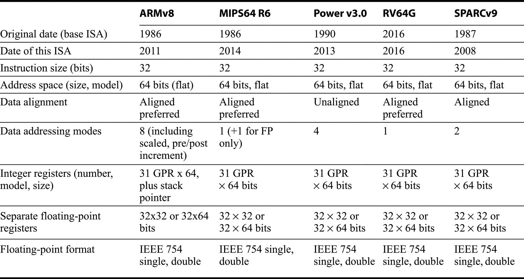
Except for the number of data address modes and some instruction set details, the integer instruction sets of these architectures are very similar. Contrast this with Figure K.29. In ARMv8, register 31 is a 0 (like register 0 in the other architectures), but when it is used in a load or store, it is the current stack pointer, a special purpose register. We can either think of SP-based addressing as a different mode (which is how the assembly mnemonics operate) or as simply a register + offset addressing mode (which is how the instruction is encoded).
There are two other important historical RISC processors that are almost identical to those in the list above: the DEC Alpha processor, which was made by Digital Equipment Corporation from 1992 to 2004 and is almost identical to MIPS64. Hewlett-Packard’s PA-RISC was produced by HP from about 1986 to 2005, when it was replaced by Itanium. PA-RISC is most closely related to the Power ISA, which emerged from the IBM Power design, itself a descendant of IBM 801.
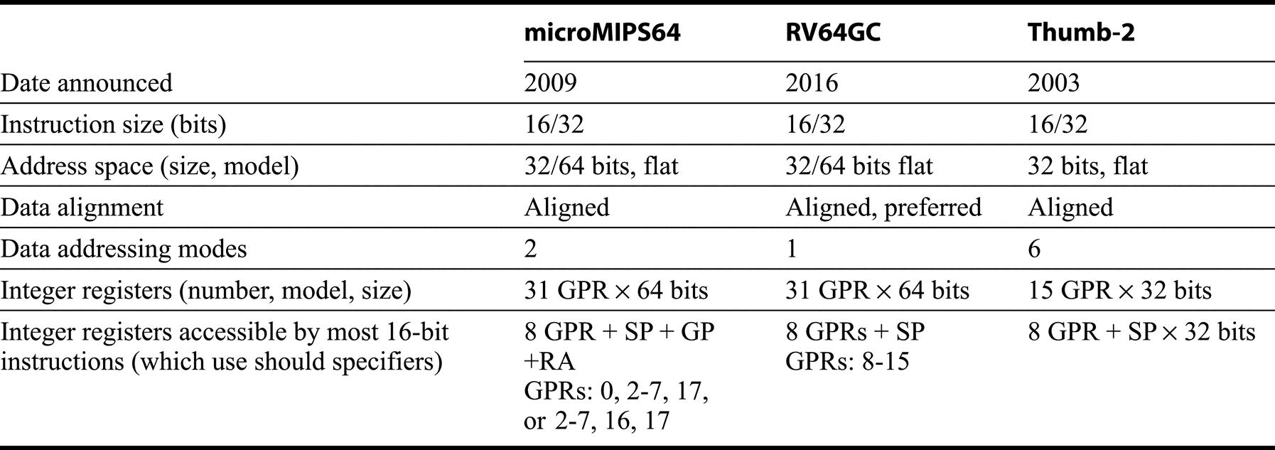
The second group is the embedded RISCs designed for lower-end applications:
- Advanced RISC Machines, Thumb-2: an 32-bit instruction set with 16-bit and 32-bit instructions. The architecture includes features from both ARMv7 and ARMv8.
- microMIPS64: a version of the MIPS64 instruction set with 16-it instructions, and
- RISC-V Compressed extension (RV64GC), a set of 16-bit instructions added to RV64G
Both RV64GC and microMIPS64 have corresponding 32-bit versions: RV32GC and microMIPS32.
Since the comparison of the base 32-bit or 64-bit desktop and server architecture will examine the differences among those ISAs, our discussion of the embedded architectures focuses on the 16-bit instructions. Figure K.2 shows that these embedded architectures are also similar. In all three, the 16-bit instructions are versions of 32-bit instructions, typically with a restricted set of registers. The idea is to reduce the code size by replacing common 32-bit instructions with 16-bit versions. For RV32GC or Thumb-2, including the 16-bit instructions yields a reduction in code size to about 0.73 of the code size using only the 32-bit ISA (either RV32G or ARMv7).
All three use 16-bit extensions of a base instruction set. Except for number of data address modes and a number of instruction set details, the integer instruction sets of these architectures are similar. Contrast this with Figure K.29. An earlier 16-bit version of the MIPS instruction set, called MIPS16, was created in 1995 and was replaced by microMIPS32 and microMIPS64. The first Thumb architecture had only 16-bit instructions and was created in 1996. Thumb-2 is built primarily on ARMv7, the 32-bit ARM instruction set; it offers 16 registers. RISC-V also defines RV32E, which has only 16 registers, includes the 16-bit instructions, and cannot have floating point. It appears that most implementations for embedded applications opt for RV32C or RV64GC.
A key difference among these three architectures is the structure of the base 32-bit ISA. In the case of RV64GC, the 32-bit instructions are exactly those of RV64G. This is possible because RISC V planned for the 16-it option from the beginning, and branch addresses and jump addresses are specified to 16-it boundaries. In the case of microMIPS64, the base ISA is MIPS64, with one change: branch and jump offsets are interpreted as 16-bit rather than 32-bit aligned. (microMIPS also uses the encoding space that was reserved in MIPS64 for user-defined instruction set extensions; such extensions are not part of the base ISA.)
Thumb-2 uses a slightly different approach. The 32-bit instructions in Thumb-2 are mostly a subset of those in ARMv7; certain features that were dropped in ARMv8 are not included (e.g., conditional execution of most instructions and the ability to write the PC as a GPR). Thumb-2 also includes a few dozen instructions introduced in ARMv8, specifically bit field manipulation, additional system instructions, and synchronization support. Thus, the 32-bit instructions in Thumb-2 constitute a unique ISA.
Earlier versions of the 16-bit instruction sets for MIPS (MIPS16) and ARM (Thumb), took the approach of creating a separate mode, invoked by a procedure call, to transfer control to a code segment that employed only 16-bit instructions.
The 16-bit instruction set was not complete and was only intended for user programs that were code-size critical.
One complication of this description is that some of the older RISCs have been extended over the years. We decided to describe the most recent versions of the architectures: ARMv8 (the 64-bit architecture AArch64), MIPS64 R6, Power v3.0, RV64G, and SPARC v9 for the desktop/server/PMD, and the 16-bit subset of the ISAs for microMIPS64, RV64GC, and Thumb-2.
The remaining sections proceed as follows. After discussing the addressing modes and instruction formats of our RISC architectures, we present the survey of the instructions in five steps:
- Instructions found in the RV64G core, described in Appendix A.
- Instructions not found in the RV64G or RV64GC but found in two or more of the other architectures. We describe and organize these by functionality, e.g. instructions that support extended integer arithmetic.
- Instruction groups unique to ARM, MIPS, Power, or SPARC, organized by function.
- Multimedia extensions of the desktop/server/PMD RISCs
- Digital signal-processing extensions of the embedded RISCs
Although the majority of the instructions in these architectures are included, we have not included every single instruction; this is especially true for the Power and ARM ISAs, which have many instructions.
Addressing Modes and Instruction Formats
Figure K.3 shows the data addressing modes supported by the desktop/server/PMD architectures. Since all, but ARM, have one register that always has the value 0 when used in address modes, the absolute address mode with limited range can be synthesized using register 0 as the base in displacement addressing. (This register can be changed by arithmetic-logical unit (ALU) operations in PowerPC, but is always zero when it is used in an address calculation.) Similarly, register indirect addressing is synthesized by using displacement addressing with an offset of 0. Simplified addressing modes is one distinguishing feature of RISC architectures.
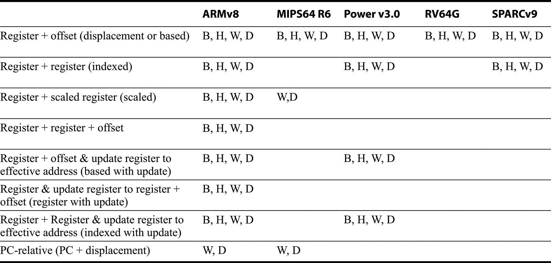
Note that ARM includes two different types of address modes with updates, one of which is included in Power.
As Figure K.4 shows, the embedded architectures restrict the registers that can be accessed with the 16-bit instructions, typically to only 8 registers, for most instructions, and a few special instructions that refer to other registers. Figure K.5 shows the data addressing modes supported by the embedded architectures in their 16-bit instruction mode. These versions of load/store instructions restrict the registers that can be used in address calculations, as well as significantly shorten the immediate fields, used for displacements.
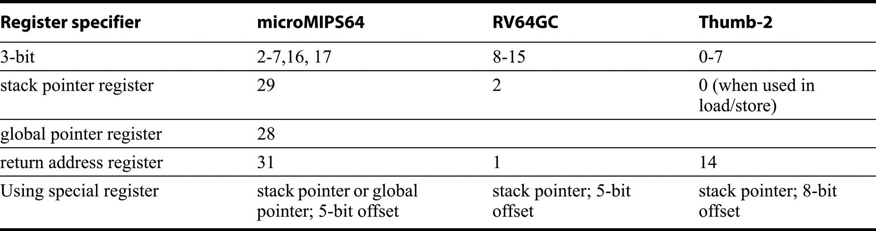
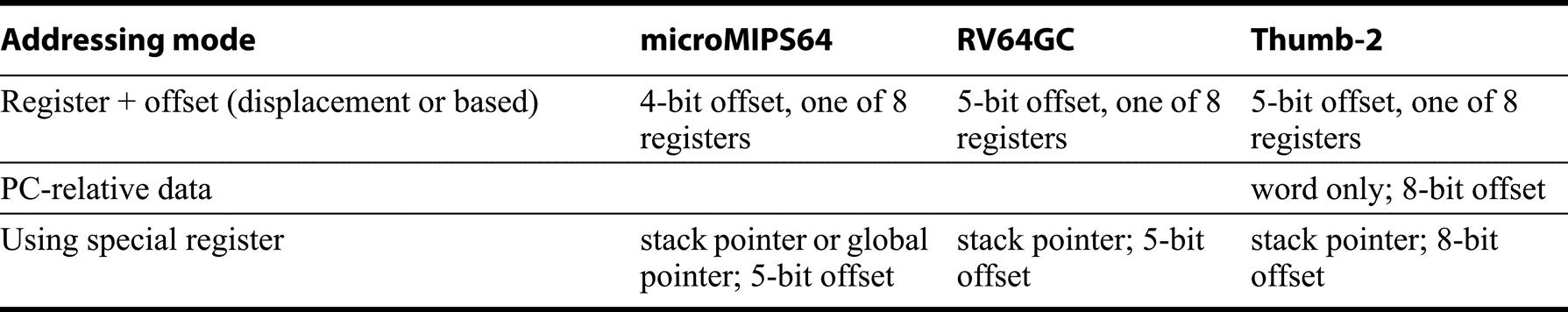
microMIPS64, RV64c, and Thumb-2 show only the modes supported in 16-bit instruction formats. The stack pointer in RV64GC and microMIPS64 is a designed GPR; it is another version of r31 is Thumb-2. In microMIPS64, the global pointer is register 30 and is used by the linkage convention to point to the global variable data pool. Notice that typically only 8 registers are accessible as base registers (and as we will see as ALU sources and destinations).
References to code are normally PC-relative, although jump register indirect is supported for returning from procedures, for case statements, and for pointer function calls. One variation is that PC-relative branch addresses are often shifted left 2 bits before being added to the PC for the desktop RISCs, thereby increasing the branch distance. This works because the length of all instructions for the desktop RISCs is 32 bits and instructions must be aligned on 32-bit words in memory. Embedded architectures and RISC V (when extended) have 16-bit-long instructions and usually shift the PC-relative address by 1 for similar reasons.
Figure K.6 shows the most important instruction formats of the desktop/server/PMD RISC instructions. Each instruction set architecture uses four primary instruction formats, which typically include 90–98% of the instructions. The register-register format is used for register-register ALU instructions, while the ALU immediate format is used for ALU instructions with an immediate operand and also for loads and stores. The branch format is used for conditional branches, and the jump/call format for unconditional branches (jumps) and procedures calls.
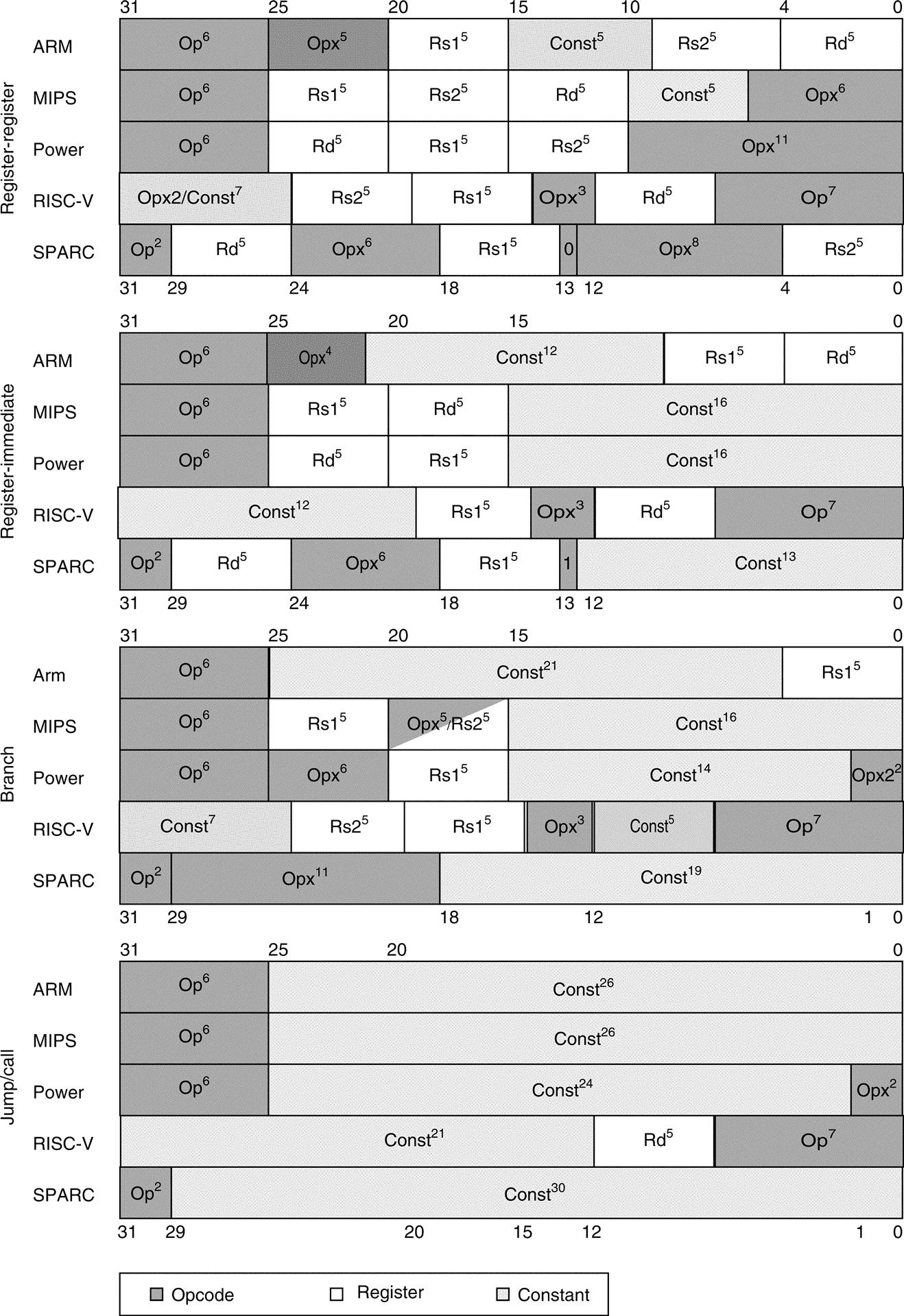
These four formats are found in all five architectures. (The superscript notation in this figure means the width of a field in bits.) Although the register fields are located in similar pieces of the instruction, be aware that the destination and two source fields are sometimes scrambled. Op = the main opcode, Opx = an opcode extension, Rd = the destination register, Rs1 = source register 1, Rs2 = source register 2, and Const = a constant (used as an immediate, address, mask, or sift amount). Although the labels on the instruction formats tell where various instructions are encoded, there are variations. For example, loads and stores, both use the ALU immediate form in MIPS. In RISC-V, loads use the ALU immediate format, while stores use the branch format.
There are a number of less frequently used instruction formats that Figure K.6 leaves out. Figure K.7 summarizes these for the desktop/server/PMD architectures.
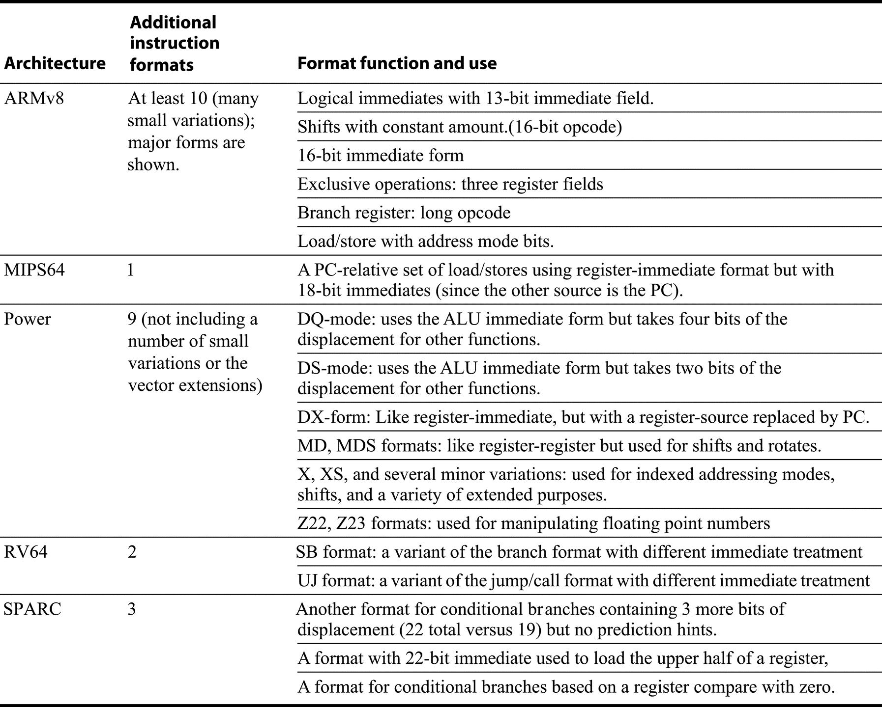
In some cases, there are formats very similar to one of the four core formats, but where a register field is used for other purposes. The Power architecture also includes a number of formats for vector operations.
Unlike, their 32-bit base architectures, the 16-bit extensions (microMIPS64, RV64GC, and Thumb-2) are focused on minimizing code. As a result, there are a larger number of instruction formats, even though there are far fewer instructions. microMIPs64 and RV64GC have eight and seven major formats, respectively, and Thumb-2 has 15. As Figure K.8 shows, these involve varying number of register operands (0 to 3), different immediate sizes, and even different size register specifiers, with a small number of registers accessible my most instructions, and fewer instructions able to access all 32 registers.
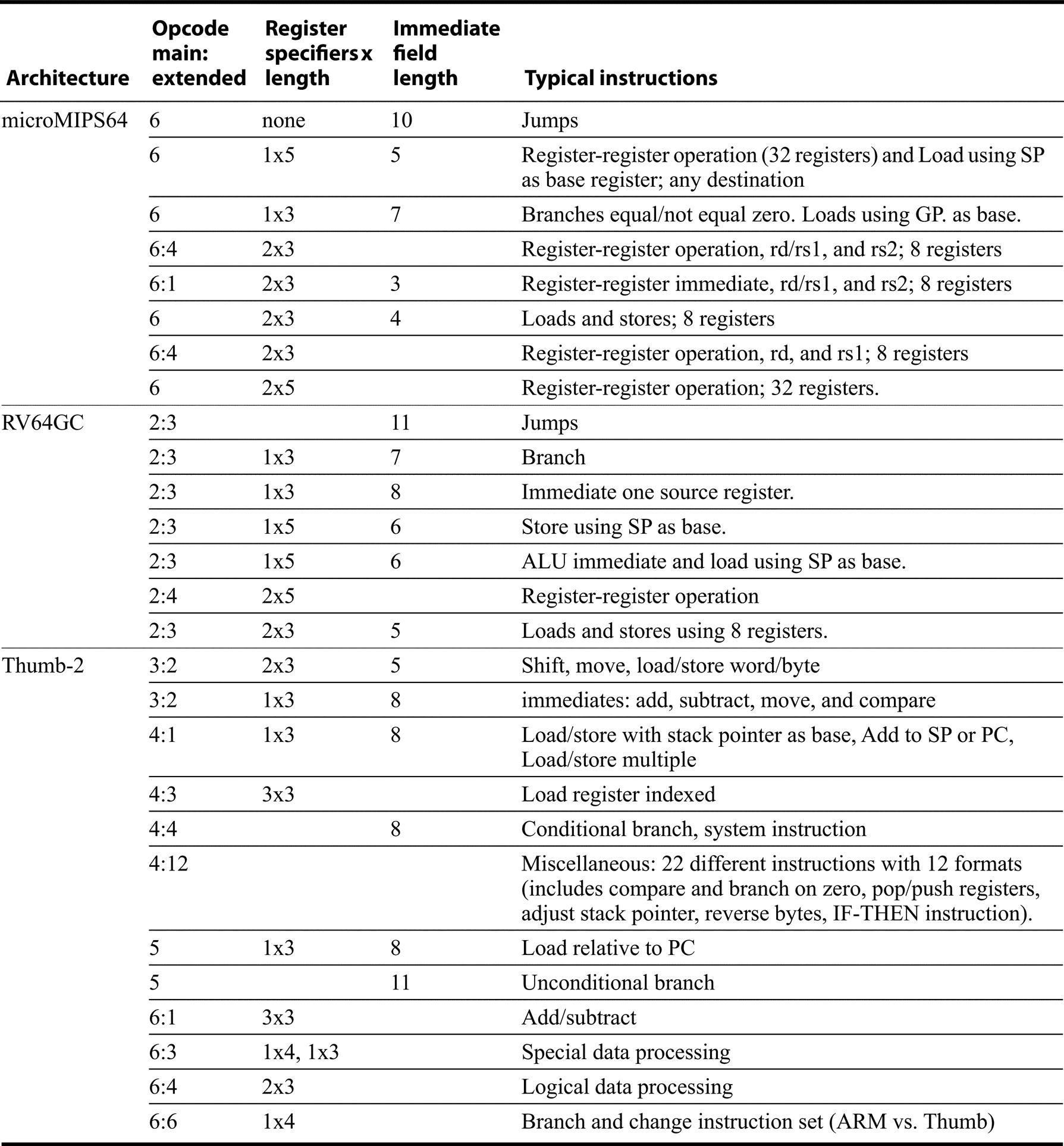
For instructions with a destination and two sources, but only two register fields, the instruction uses one of the registers as both source and destination. Note that the extended opcode field (or function field) and immediate field sometimes overlap or are identical. For RV64GC and microMIPS64, all the formats are shown; for Thumb-2, the Miscellaneous format includes 22 instructions with 12 slightly different formats; we use the extended opcode field, but a few of these instructions have immediate or register fields.
Instructions
The similarities of each architecture allow simultaneous descriptions, starting with the operations equivalent to the RISC-V 64-bit ISA.
RV64G Core Instructions
Almost every instruction found in the RV64G is found in the other architectures, as Figures K.9 through K.19 show. (For reference, definitions of the RISC-V instructions are found in Section A.9.) Instructions are listed under four categories: data transfer (Figure K.9); arithmetic, logical (Figure K.10); control (Figure K.11 and Figure K.12); and floating point (Figure K.13).
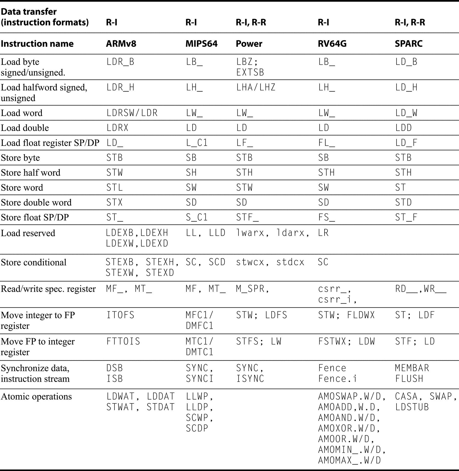
A sequence of instructions to synthesize a RV64G instruction is shown separated by semicolons. The MIPS and Power instructions for atomic operations load and conditionally store a pair of registers and can be used to implement the RV64G atomic operations with at most one intervening ALU instruction. The SPARC instructions: compare-and-swap, swap, LDSTUB provide atomic updates to a memory location and can be used to build the RV64G instructions. The Power3 instructions provide all the functionality, as the RV64G instructions, depending on a function field.
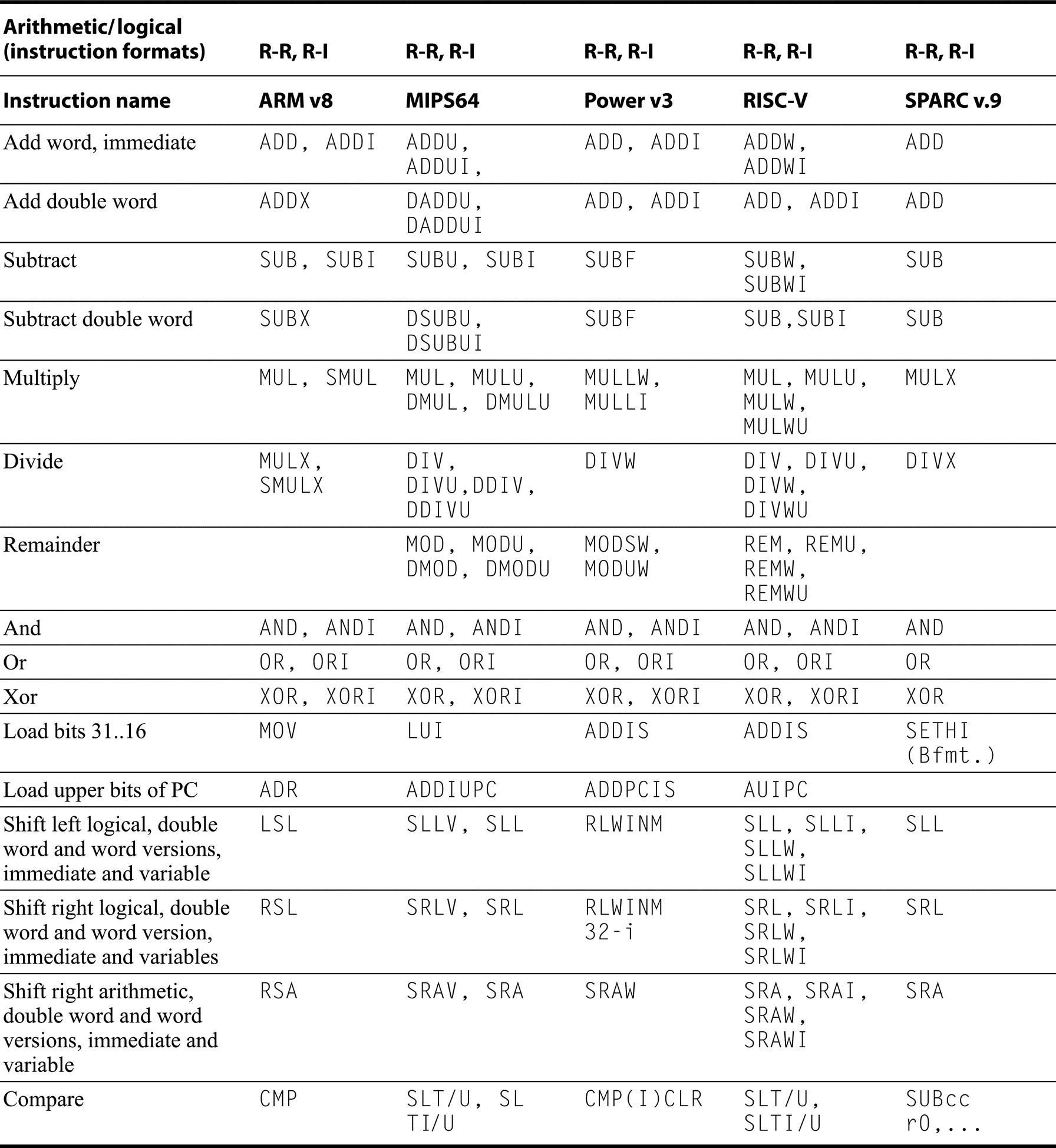
MIPS also provides instructions that trap on arithmetic overflow, which are synthesized in other architectures with multiple instructions. Note that in the “Arithmetic/logical” category all machines but SPARC use separate instruction mnemonics to indicate an immediate operand; SPARC offers immediate versions of these instructions but uses a single mnemonic. (Of course, these are separate opcodes!)
Integer compare on SPARC is synthesized with an arithmetic instruction that sets the condition codes using r0 as the destination.
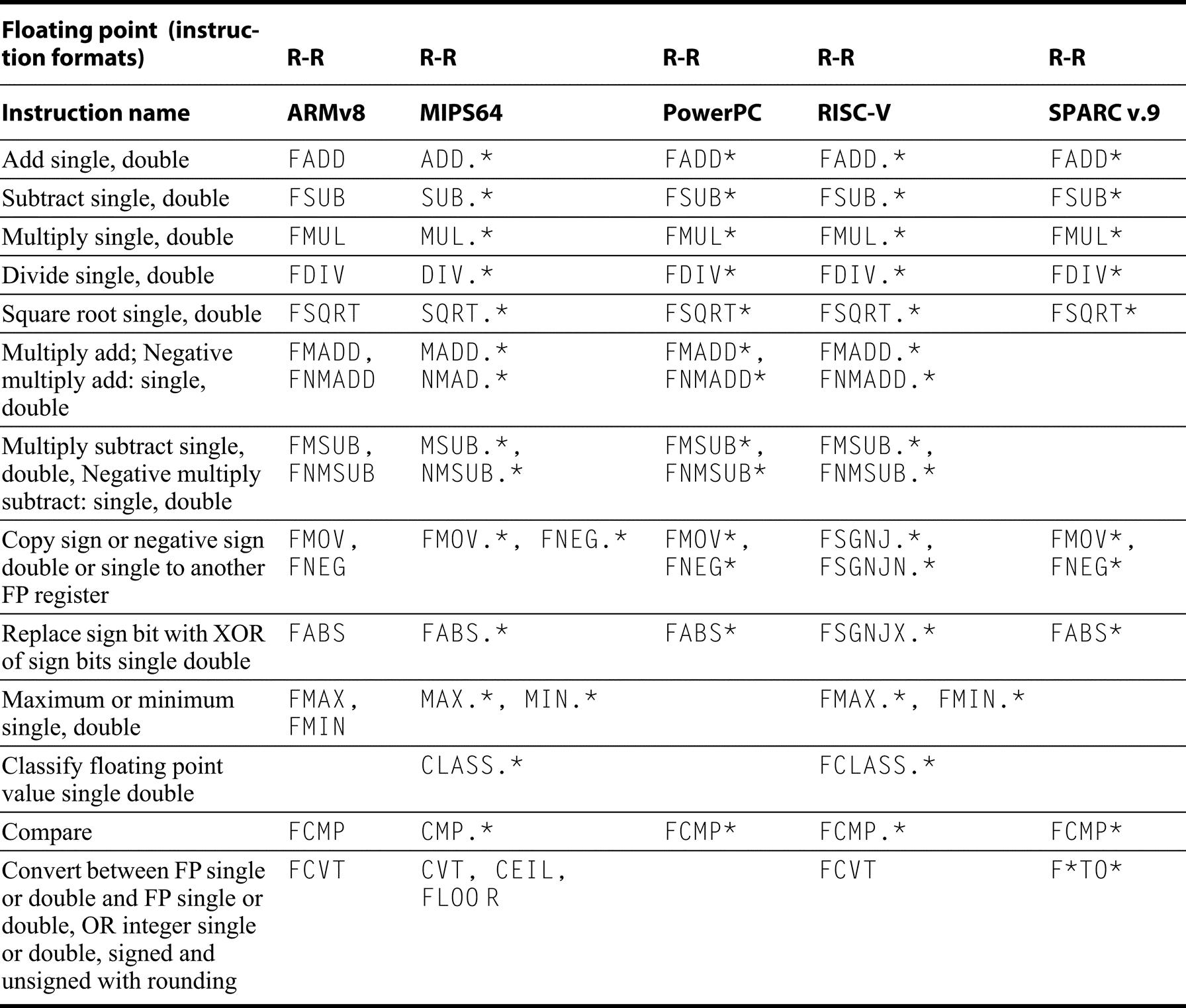
ARMv8 uses the same assembly mnemonic for single and double precision; the register designator indicates the precision. “*” is used as an abbreviation for S or D. For floating point compares all conditions: equal, not equal, less than, and less-then or equal are provided. Moves operate in both directions from/to integer registers. Classify sets a register based on whether the floating point quantity is plus or minus infinity, denorm, +/ − 0, etc.). The sign-injection instructions take two operands, but are primarily used to form floating point move, negate, and absolute value, which are separate instructions in the other ISAs.
If a RV64G core instruction requires a short sequence of instructions in other architectures, these instructions are separated by semicolons in Figure K.9 through Figure K.13. (To avoid confusion, the destination register will always be the leftmost operand in this appendix, independent of the notation normally used with each architecture.).
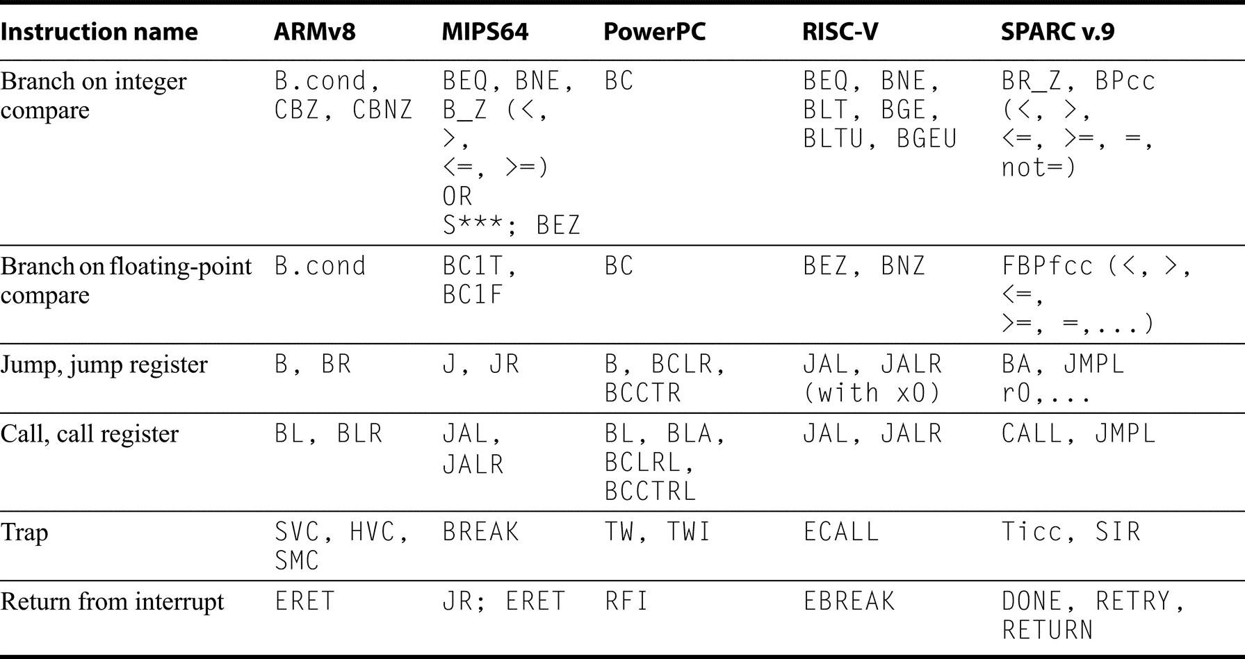
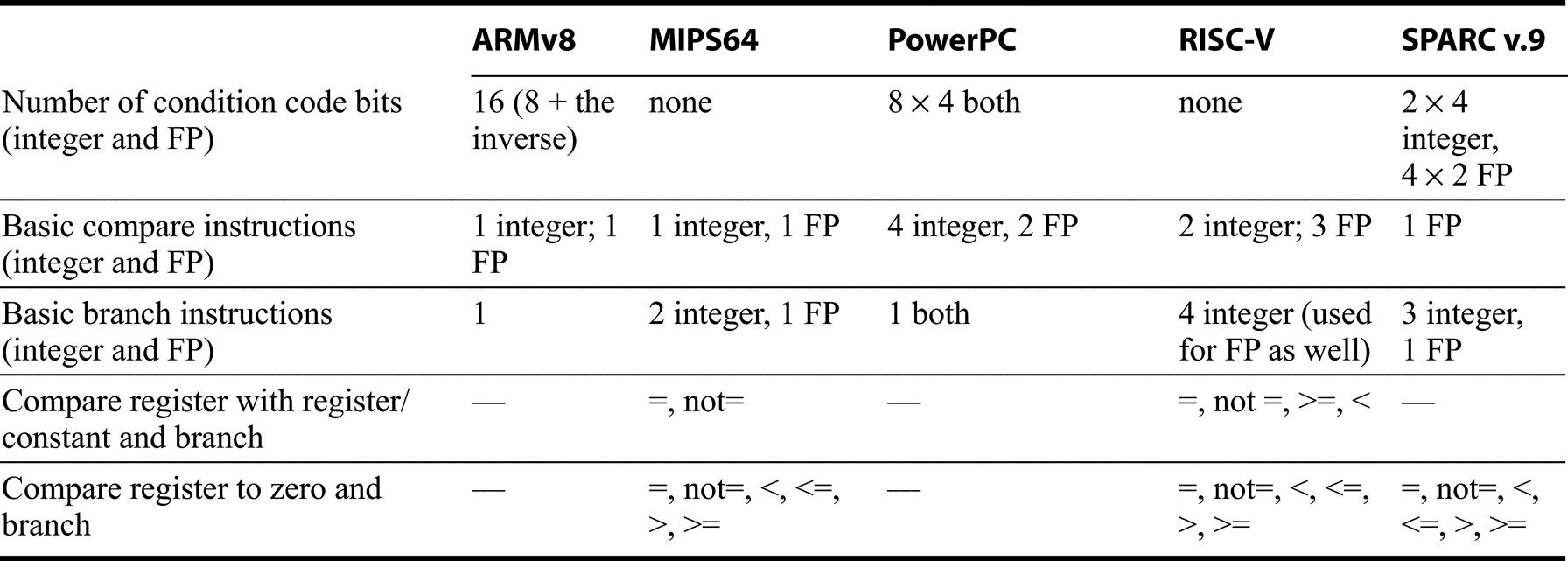
Compare and Conditional Branch
Every architecture must have a scheme for compare and conditional branch, but despite all the similarities, each of these architectures has found a different way to perform the operation! Figure K.11 summarizes the control instructions, while Figure K.12 shows details of how conditional branches are handled. SPARC uses the traditional four condition code bits stored in the program status word: negative, zero, carry, and overflow. They can be set on any arithmetic or logical instruction; unlike earlier architectures, this setting is optional on each instruction. An explicit option leads to fewer problems in pipelined implementation. Although condition codes can be set as a side effect of an operation, explicit compares are synthesized with a subtract using r0 as the destination. SPARC conditional branches test condition codes to determine all possible unsigned and signed relations. Floating point uses separate condition codes to encode the EEE 754 conditions, requiring a floating-point compare instruction. Version 9 expanded SPARC branches in four ways: a separate set of condition codes for 64-bit operations; a branch that tests the contents of a register and branches if the value is =, not =, <, <=, >=, or <= 0; three more sets of floating-point condition codes; and branch instructions that encode static branch prediction.
Power also uses four condition codes: less than, greater than, equal, and summary overflow, but it has eight copies of them. This redundancy allows the Power instructions to use different condition codes without conflict, essentially giving Power eight extra 4-bit registers. Any of these eight condition codes can be the target of a compare instruction, and any can be the source of a conditional branch. The integer instructions have an option bit that behaves as if the integer is followed by a compare to zero that sets the first condition “register.” Power also lets the second “register” be optionally set by floating-point instructions. PowerPC provides logical operations among these eight 4-bit condition code registers (CRAND, CROR, CRXOR, CRNAND, CRNOR, CREQV), allowing more complex conditions to be tested by a single branch. Finally, Power includes a set of branch count registers, that are automatically decremented when tested, and can be used in a branch condition. There are also special instructions for moving from/to the condition register.
RISC-V and MIPS are most similar. RISC-V uses a compare and branch with a full set of arithmetic comparisons. MIPS also uses compare and branch, but the comparisons are limited to equality and tests against zero. This limited set of conditions simplifies the branch determination (since an ALU operation is not required to test the condition), at the cost of sometimes requiring the use of a set-on-less-than instruction (SLT, SLTI, SLTU, SLTIU), which compares two operands and then set the destination register to 1 if less and to 0 otherwise. Figure K.12 provides additional details on conditional branch. RISC-V floating point comparisons sets an integer register to 0 or 1, and then use conditional branches on that content.MIPS also uses separate floating-point compare, which sets a floating point register to 0 or 1, which is then tested by a floating-point conditional branch.
ARM is similar to SPARC, in that it provides four traditional condition codes that are optionally set. CMP subtracts one operand from the other and the difference sets the condition codes. Compare negative (CMN) adds one operand to the other, and the sum sets the condition codes. TST performs logical AND on the two operands to set all condition codes but overflow, while TEQ uses exclusive OR to set the first three condition codes. Like SPARC, the conditional version of the ARM branch instruction tests condition codes to determine all possible unsigned and signed relations. ARMv8 added both bit-test instructions and also compare and branch against zero. Floating point compares on ARM, set the integer condition codes, which are used by the B.cond instruction.
As Figure K.13 shows the floating point support is similar on all five architectures.
RV64GC Core 16-bit Instructions
Figures K.14 through K.17 summarize the data transfer, ALU, and control instructions for our three embedded processors: microMIPS64, RV64GC, and Thumb-2. Since these architectures are all based on 32-bit or 64-bit versions of the full architecture, we focus our attention on the functionality implemented by the 16-bit instructions. Since floating point is optional, we do not include it. I

Rather than show the instruction name, where appropriate, we show the number of registers that can the base register for the address calculation, followed by the number of registers that can be the destination for a load or the source for a store, and finally, the size of the immediate used for address calculation. For example: 8; 8; 5 for a load means that there are 8 possible base registers, 8 possible destination registers for the load, and a 5-bit offset for the address calculation. For a store, 8; 8; 5, specifies that the source of the value to store comes from one of 8 registers. Remember that Thumb-2 also has 32-bit instructions (although not the full ARMv8 set) and that RV64GC and microMIPS64 have the full set of 32-bit instructions in RV64I or MIPS64.
Instructions: Common Extensions beyond RV64G
Figures K.15 through K.18 list instructions not found in Figures K.9 through K.13 in the same four categories (data transfer, ALU, and control. The only significant floating point extension is the reciprocal instruction, which both MIPS64 and Power support. Instructions are put in these lists if they appear in more than one of the standard architectures. Recall that Figure K.3 on page 6 showed the address modes supported by the various instruction sets. All three processors provide more address modes than provided by RV64G. The loads and stores using these additional address modes are not shown in Figure K.17, but are effectively additional data transfer instructions. This means that ARM has 64 additional load and store instructions, while Power3 has 12, and MIPS64 and SPARVv9 each have 4.
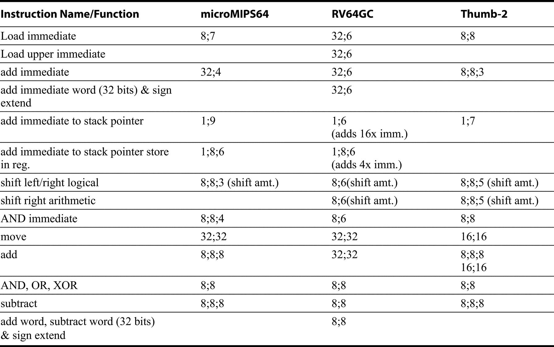
An entry shows the number of register sources/destinations, followed by the size of the immediate field, if it exists for that instruction. The add to stack pointer with scaled immediate instructions are used for adjusting the stack pointer and creating a pointer to a location on the stack. In Thumb, the add has two forms one with three operands from the 8-register subset (Lo) and one with two operands but any of 16-registers.
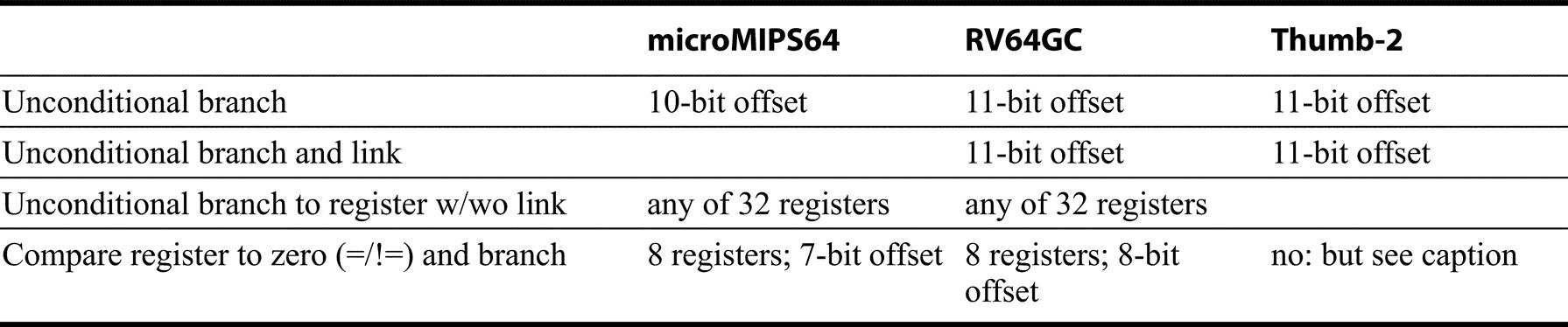
A blank indicates that the instruction does not exist. Thumb-2 uses 4 condition code bits; it provides a conditional branch that tests the 4-bit condition code and has a branch offset of 8 bits.
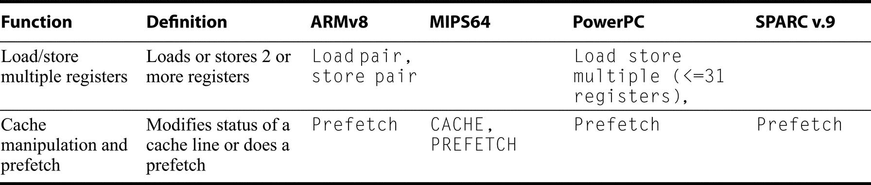
SPARC requires memory accesses to be aligned, while the other architectures support unaligned access, albeit, often with major performance penalties. The other architectures do not require alignment, but may use slow mechanisms to handle unaligned accesses.MIPS provides a set of instructions to handle misaligned accesses: LDL and LDR (load double left and load double right instructions) work as a pair to load a misaligned word; the corresponding store instructions perform the inverse. The Prefetch instruction causes a cache prefetch, while CACHE provides limited user control over the cache state.
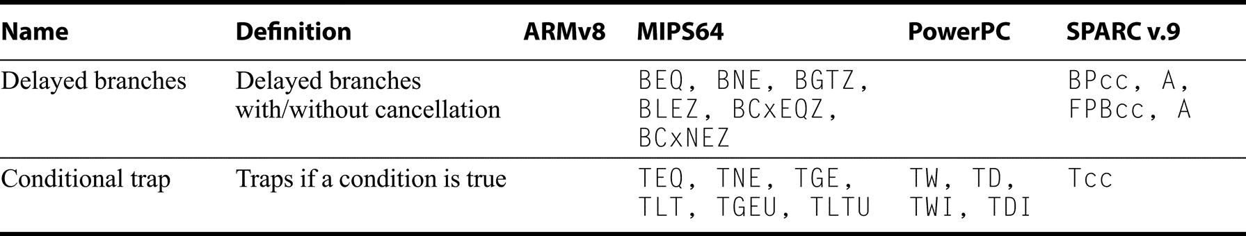
MIPS64 Release 6 has nondelayed and normal delayed branches, while SPARC v.9 has delayed branches with cancellation based on the static prediction.
To accelerate branches, modern processors use dynamic branch prediction (see Section 3.3). Many of these architectures in earlier versions supported delayed branches, although they have been dropped or largely eliminated in later versions of the architecture, typically by offering a nondelayed version, as the preferred conditional branch. The SPARC “annulling” branch is an optimized form of delayed branch that executes the instruction in the delay slot only if the branch is taken; otherwise, the instruction is annulled. This means the instruction at the target of the branch can safely be copied into the delay slot since it will only be executed if the branch is taken. The restrictions are that the target is not another branch and that the target is known at compile time. (SPARC also offers a nondelayed jump because an unconditional branch with the annul bit set does not execute the following instruction.).
In contrast to the differences among the full ISAs, the 16-bit subsets of the three embedded ISAs have essentially no significant differences other than those described in the earlier figures (e.g. size of immediate fields, uses of SP or other registers, etc.).
Now that we have covered the similarities, we will focus on the unique features of each architecture. We first cover the desktop/server RISCs, ordering them by length of description of the unique features from shortest to longest, and then the embedded RISCs.
Instructions Unique to MIPS64 R6
MIPS has gone through six generations of instruction sets. Generations 1–4 mostly added instructions. Release 6 eliminated many older instructions but also provided support for nondelayed branches and misaligned data access. Figure K.19 summarizes the unique instructions in MIPS64 R6.
Instructions Unique to SPARC v.9
Several features are unique to SPARC. We review the major figures and then summarize those and small differences in a figure.
Register Windows
The primary unique feature of SPARC is register windows, an optimization for reducing register traffic on procedure calls. Several banks of registers are used, with a new one allocated on each procedure call. Although this could limit the depth of procedure calls, the limitation is avoided by operating the banks as a circular buffer. The knee of the cost-performance curve seems to be six to eight banks; programs with deeper call stacks, would need to save and restore the registers to memory.
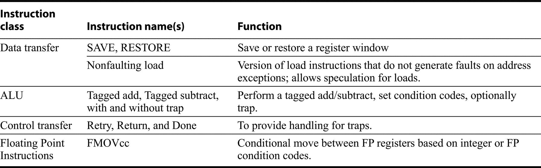
SPARC can have between 2 and 32 windows, typically using 8 registers each for the globals, locals, incoming parameters, and outgoing parameters. (Given that each window has 16 unique registers, an implementation of SPARC can have as few as 40 physical registers and as many as 520, although most have 128 to 136, so far.) Rather than tie window changes with call and return instructions, SPARC has the separate instructions SAVE and RESTORE. SAVE is used to “save” the caller’s window by pointing to the next window of registers in addition to performing an add instruction. The trick is that the source registers are from the caller’s window of the addition operation, while the destination register is in the callee’s window. SPARC compilers typically use this instruction for changing the stack pointer to allocate local variables in a new stack frame. RESTORE is the inverse of SAVE, bringing back the caller’s window while acting as an add instruction, with the source registers from the callee’s window and the destination register in the caller’s window. This automatically deallocates the stack frame. Compilers can also make use of it for generating the callee’s final return value.
The danger of register windows is that the larger number of registers could slow down the clock rate. This was not the case for early implementations. The SPARC architecture (with register windows) and the MIPS R2000 architecture (without) have been built in several technologies since 1987. For several generations the SPARC clock rate has not been slower than the MIPS clock rate for implementations in similar technologies, probably because cache access times dominate register access times in these implementations. With the advent of multiple issue, which requires many more register ports, as will as register renaming or reorder buffers, register windows posed a larger penalty.Register windows were a feature of the original Berkeley RISC designs, and their inclusion in SPARC was inspired by those designs. Tensilica is the only other major architecture in use today employs them, and they were not included in the RISC-V ISA.
Fast Traps
SPARCv9 includes support to make traps fast. It expands the single level of traps to at least four levels, allowing the window overflow and underflow trap handlers to be interrupted. The extra levels mean the handler does not need to check for page faults or misaligned stack pointers explicitly in the code, thereby making the handler faster. Two new instructions were added to return from this multilevel handler: RETRY (which retries the interrupted instruction) and DONE (which does not). To support user-level traps, the instruction RETURN will return from the trap in nonprivileged mode.
Support for LISP and Smalltalk
The primary remaining arithmetic feature is tagged addition and subtraction. The designers of SPARC spent some time thinking about languages like LISP and Smalltalk, and this influenced some of the features of SPARC already discussed: register windows, conditional trap instructions, calls with 32-bit instruction addresses, and multi-word arithmetic (see Taylor et al. [1986] and Ungar et al. [1984]). A small amount of support is offered for tagged data types with operations for addition, subtraction, and hence comparison. The two least-significant bits indicate whether the operand is an integer (coded as 00), so TADDcc and TSUBcc set the overflow bit if either operand is not tagged as an integer or if the result is too large. A subsequent conditional branch or trap instruction can decide what to do. (If the operands are not integers, software recovers the operands, checks the types of the operands, and invokes the correct operation based on those types.) It turns out that the misaligned memory access trap can also be put to use for tagged data, since loading from a pointer with the wrong tag can be an invalid access. Figure K.20 shows both types of tag support.
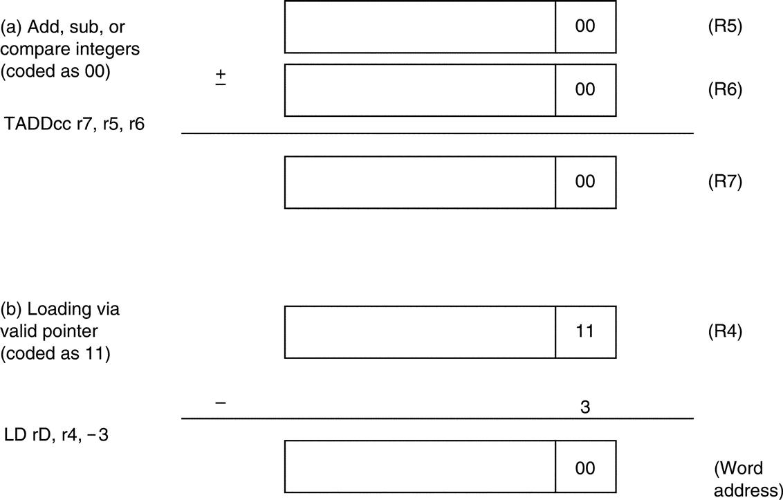
(a) Integer arithmetic, which takes a single cycle as long as the operands and the result are integers. (b) The misaligned trap can be used to catch invalid memory accesses, such as trying to use an integer as a pointer. For languages with paired data like LISP, an offset of –3 can be used to access the even word of a pair (CAR) and + 1 can be used for the odd word of a pair (CDR).
Figure K.21 summarizes the additional instructions mentioned above as well as several others.
Instructions Unique to ARM
Earlier versions of the ARM architecture (ARM v6 and v7) had a number of unusual features including conditional execution of all instructions, and making the PC a general purpose register. These features were eliminated with the arrival of ARMv8 (in both the 32-bit and 64-bit ISA). What remains, however, is much of the complexity, at least in terms of the size of the instruction set. As Figure K.3 on page 6 shows, ARM has the most addressing modes, including all those listed in the table; remember that these addressing modes add dozens of load/store instructions compared to RVG, even though they are not listed in the table that follows. As Figure K.6 on page 8 shows, ARMv8 also has by far the largest number of different instruction formats, which reflects a variety of instructions, as well as the different addressing modes, some of which are applicable to some loads and stores but not others.
Most ARMv8 ALU instructions allow the second operand to be shifted before the operation is completed. This extends the range of immediates, but operand shifting is not limited to immediates. The shift options are shift left logical, shift right logical, shift right arithmetic, and rotate right. In addition, as in Power3, most ALU instructions can optionally set the condition flags. Figure K.22 includes the additional instructions, but does not enumerate all the varieties (such as optional setting of the condition flags); see the caption for more detail. While conditional execution of all instructions was eliminated, ARMv8 provides a number of conditional instructions beyond the conditional move and conditional set, mentioned earlier.
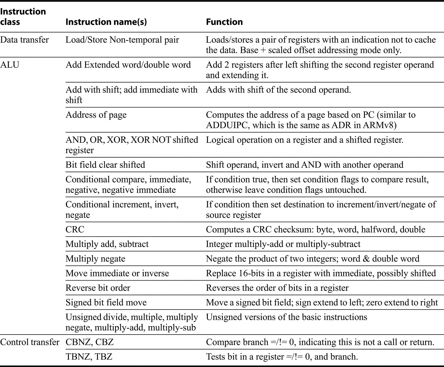
Unless noted the instruction is available in a word and double word format, if there is a difference. Most of the ALU instructions can optionally set the condition codes; these are not included as separate instructions here or in earlier tables.
Instructions Unique to Power3
Power3 is the result of several generations of IBM commercial RISC machines—IBM RT/PC, IBM Power1, and IBM Power2, and the PowerPC development, undertaken primarily by IBM and Motorola. First, we describe branch registers and the support for loop branches. Figure K.23 then lists the other instructions provided only in Power3.

Rotate instructions have two forms: one that sets a condition register and one that does not. There are a set of string instructions that load up to 32 bytes from an arbitrary address to a set of registers. These instructions will be phased out in future implementations, and hence we just mention them here.
Branch Registers: Link and Counter
Rather than dedicate one of the 32 general-purpose registers to save the return address on procedure call, Power3 puts the address into a special register called the link register. Since many procedures will return without calling another procedure, link doesn’t always have to be saved away. Making the return address a special register makes the return jump faster since the hardware need not go through the register read pipeline stage for return jumps.
In a similar vein, Power3 has a count register to be used in for loops where the program iterates for a fixed number of times. By using a special register the branch hardware can determine quickly whether a branch based on the count register is likely to branch, since the value of the register is known early in the execution cycle. Tests of the value of the count register in a branch instruction will automatically decrement the count register.
Given that the count register and link register are already located with the hardware that controls branches, and that one of the problems in branch prediction is getting the target address early in the pipeline (see Appendix C), the Power architects decided to make a second use of these registers. Either register can hold a target address of a conditional branch. Thus, PowerPC supplements its basic conditional branch with two instructions that get the target address from these registers (BCLR, BCCTR). Figure K.23 shows the several dozen instructions that have been added; note that there is an extensive facility for decimal floating point, as well.
Instructions: Multimedia Extensions of the Desktop/Server RISCs
Support for multimedia and graphics operations developed in several phases, beginning in 1996 with Intel MMX, MIPS MDMX, and SPARC VIS. As described in Section 4.3, which we assume the reader has read, these extensions allowed a register to be treated as multiple independent small integers (8 or 16 bits long) with arithmetic and logical operations done in parallel on all the items in a register. These initial SIMD extensions, sometimes called packed SIMD, were further developed after 2000 by widening the registers, partially or totally separating them from the general purpose or floating pointer registers, and by adding support for parallel floating point operations. RISC-V has reserved an extension for such packed SIMD instructions, but the designers have opted to focus on a true vector extension for the present. The vector extension RV64V is a vector architecture, and, as Section 4.3 points out, a true vector instruction set is considerably more general, and can typically perform the operations handled by the SIMD extensions using vector operations.
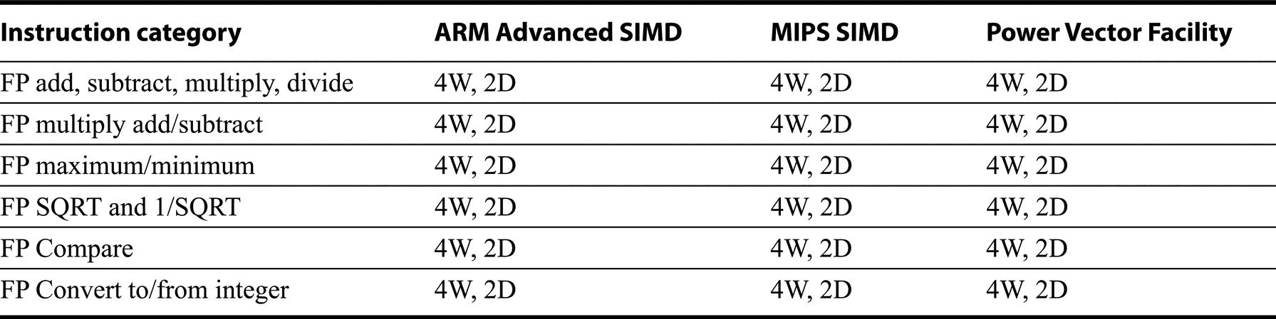
Figure K.24 shows the basic structure of the SIMD extensions in ARM, MIPS, Power, and SPARC. Note the difference in how the SIMD “vector registers” are structured: repurposing the floating point, extending the floating point, or adding additional registers. Other key differences include support for FP as well as integers, support for 128-bit integers, and provisions for immediate fields as operands in integer and logical operations. Standard load and store instructions are used for moving data from the SIMD registers to memory with special extensions to handle moving less than a full SIMD register. SPARC VIS, which was one of the earliest ISA extensions for graphics, is much more limited: only add, subtract, and multiply are included, there is no FP support, and only limited instructions for bit element operations; we include it in Figure K.24 but will not be going into more detail.
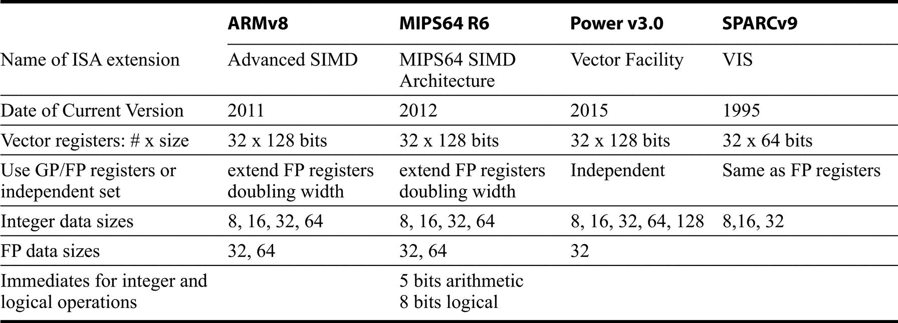
In addition to the vector facility, The last row states whether the SIMD instruction set supports immediates (e.g, add vector immediate or AND vector immediate); the entry states the size of immediates for those ISAs that support them. Note that the fact that an immediate is present is encoded in the opcode space, and could alternatively be added to the next table as additional instructions. Power 3 has an optional Vector-Scalar Extension. The Vector-Scalar Extension defines a set of vector registers that overlap the FP and normal vector registers, eliminating the need to move data back and forth to the vector registers. It also supports double precision floating point operations.
Figure K.25 shows the arithmetic instructions included in these SIMD extensions; only those appearing in at least two extensions are included. MIPS SIMD includes many other instructions, as does the Power 3 Vector-Scalar extension, which we do not cover. One frequent feature not generally found in general-purpose microprocessors is saturating operations. Saturation means that when a calculation overflows the result is set to the largest positive number or most negative number, rather than a modulo calculation as in two’s complement arithmetic. Commonly found in digital signal processors (see the next subsection), these saturating operations are helpful in routines for filtering. Another common extension are instructions for accumulating values within a single register; the dot product instruction an the maximum/minimum instructions are typical examples.
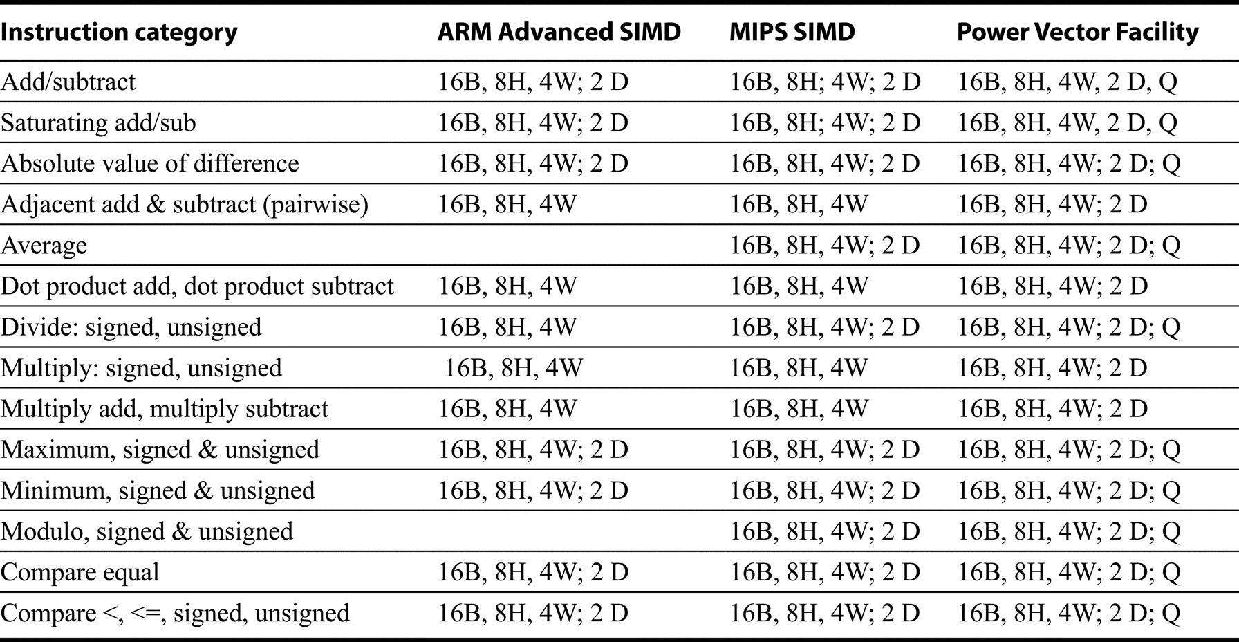
B stands for byte (8 bits), H for half word (16 bits), and W for word (32 bits), D for double word (64 bits), and Q for quad word (128 bits). Thus, 8B means an operation on 8 bytes in a single instruction. Note that some instructions--such as adjacent add/subtract, or multiply-produce results that are twice the width of the inputs (e.g. multiply on 16 bytes produces 8 halfword results). Dot product is a multiply and accumulate. The SPARC VIS instructions are aimed primarily at graphics and are structured accordingly.
In addition to the arithmetic instructions, the most common additions are logical and bitwise operations and instructions for doing version of permutations and packing elements into the SIMD registers. These additions are summarized in Figure K.26, Lastly, all three extensions support SIMD FP operations, as summarized in Figure K.27.
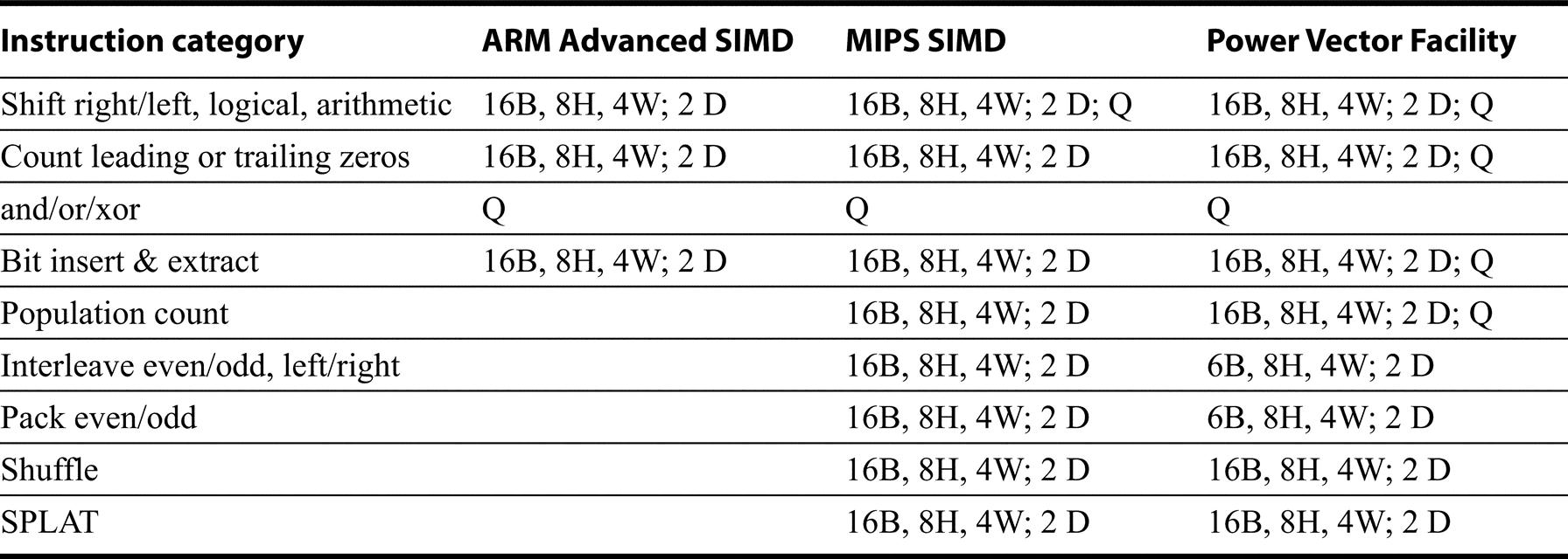
When there is a single operand the instruction applies to the entire register; for logical operations there is no difference. Interleave puts together the elements (all even, odd, leftmost or rightmost) from two different registers to create one value; it can be used for unpacking. Pack moves the even or odd elements from two different registers to the leftmost and rightmost halves of the result. Shuffle creates a from two registers based on a mask that selects which source for each item. SPLAT copies a value into each item in a register.
Instructions: Digital Signal-Processing Extensions of the Embedded RISCs
Both Thumb2 and microMIPS32 provide instructions for DSP (Digital Signal Processing) and multimedia operations. In Thumb2, these are part of the core instruction set; in microMIPS32, they are part of the DSP extension. These extensions, which are encoded as 32-bit instructions, are less extensive than the multimedia and graphics support provided in the SIMD/Vector extensions of MIPS64 or ARMv8 (AArch64). Like those more comprehensive extensions, the ones in Thumb2 and microMIPS32 also rely on packed SIMD, but they use the existing integer registers, with a small extension to allow a wide accumulator, and only operate on integer data. RISC-V has specified that the “P” extension will support packed integer SIMD using the floating point registers, but at the time of publication, the specification was not completed.
DSP operations often include linear algebra functions and operations such as convolutions; these operations produce intermediate results that will be larger than the inputs. In Thumb2, this is handled by a set of operations that produce 64-bit results using a pair of integer registers. In microMIPS32 DSP, there are 4 64-bit accumulator registers, including the Hi-Lo register, which is already exists for doing integer multiply and divide. Both architectures provide parallel arithmetic using bytes, halfwords, and words, as in the multimedia extensions in ARMv8 and MIPS64. In addition, the MIPS DSP extension handles fractional data, such data is heavily used in DSP operations. Fractional data items have a sign bit and the remaining bits are used to represent the fraction, providing a range of values from -1.0 to 0.9999 (in decimal). MIPS DSP supports two fractional data sizes Q15 and Q31 each with one sign bit and 15 or 31 bits of fraction.
Figure K.28 shows the common operations using the same notation as was used in Figure K.25. Remember that the basic 32-bit instruction set provides additional functionality, including basic arithmetic, logical, and bit manipulation.

A blank indicates that the operation is not supported as a single instruction. Byte quantities are usually unsigned. Complex multiplication step implements multiplication of complex numbers where each component is a Q15 value. ARM uses its standard condition register, while MIPS adds a set of condition bits as part of the state in the DSP extension.
Concluding Remarks
This survey covers the addressing modes, instruction formats, and almost all the instructions found in 8 RISC architectures. Although the later sections concentrate on the differences, it would not be possible to cover 8 architectures in these few pages if there were not so many similarities. In fact, we would guess that more than 90% of the instructions executed for any of these architectures would be found in Figures K.9 through K.13. To contrast this homogeneity, Figure K.29 gives a summary for four architectures from the 1970s in a format similar to that shown in Figure K.1. (Since it would be impossible to write a single section in this style for those architectures, the next three sections cover the 80x86, VAX, and IBM 360/370.) In the history of computing, there has never been such widespread agreement on computer architecture as there has been since the RISC ideas emerged in the 1980s.
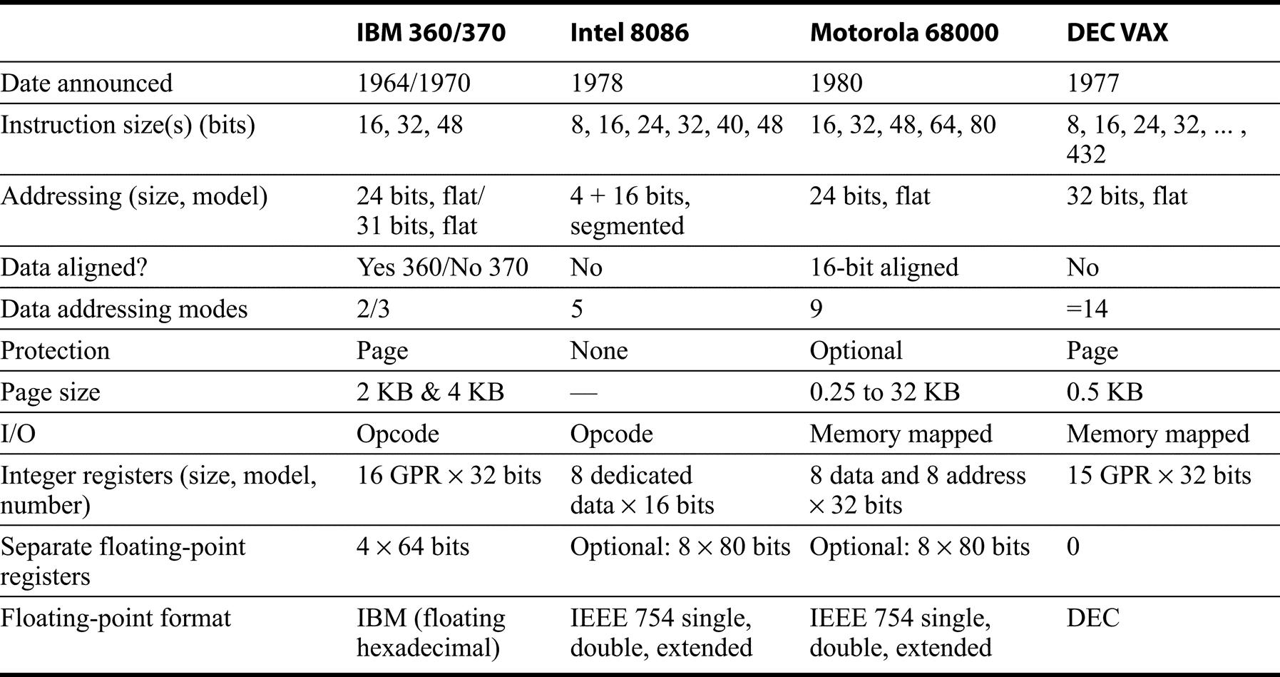
Unlike the architectures in Figure K.1, there is little agreement between these architectures in any category. (See Section K.3 for more details on the 80x86 and Section K.4 for a description of the VAX.)
K.3 The Intel 80x86
Introduction
MIPS was the vision of a single architect. The pieces of this architecture fit nicely together and the whole architecture can be described succinctly. Such is not the case of the 80x86: It is the product of several independent groups who evolved the architecture over 20 years, adding new features to the original instruction set as you might add clothing to a packed bag. Here are important 80x86 milestones:
- 1978—The Intel 8086 architecture was announced as an assembly language–compatible extension of the then-successful Intel 8080, an 8-bit microprocessor. The 8086 is a 16-bit architecture, with all internal registers 16 bits wide. Whereas the 8080 was a straightforward accumulator machine, the 8086 extended the architecture with additional registers. Because nearly every register has a dedicated use, the 8086 falls somewhere between an accumulator machine and a general-purpose register machine, and can fairly be called an extended accumulator machine.
- 1980—The Intel 8087 floating-point coprocessor is announced. This architecture extends the 8086 with about 60 floating-point instructions. Its architects rejected extended accumulators to go with a hybrid of stacks and registers, essentially an extended stack architecture: A complete stack instruction set is supplemented by a limited set of register-memory instructions.
- 1982—The 80286 extended the 8086 architecture by increasing the address space to 24 bits, by creating an elaborate memory mapping and protection model, and by adding a few instructions to round out the instruction set and to manipulate the protection model. Because it was important to run 8086 programs without change, the 80286 offered a real addressing mode to make the machine look just like an 8086.
- 1985—The 80386 extended the 80286 architecture to 32 bits. In addition to a 32-bit architecture with 32-bit registers and a 32-bit address space, the 80386 added new addressing modes and additional operations. The added instructions make the 80386 nearly a general-purpose register machine. The 80386 also added paging support in addition to segmented addressing (see Chapter 2). Like the 80286, the 80386 has a mode to execute 8086 programs without change.
This history illustrates the impact of the “golden handcuffs” of compatibility on the 80x86, as the existing software base at each step was too important to jeopardize with significant architectural changes. Fortunately, the subsequent 80486 in 1989, Pentium in 1992, and P6 in 1995 were aimed at higher performance, with only four instructions added to the user-visible instruction set: three to help with multiprocessing plus a conditional move instruction.
Since 1997 Intel has added hundreds of instructions to support multimedia by operating on many narrower data types within a single clock (see Appendix A). These SIMD or vector instructions are primarily used in hand-coded libraries or drivers and rarely generated by compilers. The first extension, called MMX, appeared in 1997. It consists of 57 instructions that pack and unpack multiple bytes, 16-bit words, or 32-bit double words into 64-bit registers and performs shift, logical, and integer arithmetic on the narrow data items in parallel. It supports both saturating and nonsaturating arithmetic. MMX uses the registers comprising the floating-point stack and hence there is no new state for operating systems to save.
In 1999 Intel added another 70 instructions, labeled SSE, as part of Pentium III. The primary changes were to add eight separate registers, double their width to 128 bits, and add a single-precision floating-point data type. Hence, four 32-bit floating-point operations can be performed in parallel. To improve memory performance, SSE included cache prefetch instructions plus streaming store instructions that bypass the caches and write directly to memory.
In 2001, Intel added yet another 144 instructions, this time labeled SSE2. The new data type is double-precision arithmetic, which allows pairs of 64-bit floating-point operations in parallel. Almost all of these 144 instructions are versions of existing MMX and SSE instructions that operate on 64 bits of data in parallel. Not only does this change enable multimedia operations, but it also gives the compiler a different target for floating-point operations than the unique stack architecture. Compilers can choose to use the eight SSE registers as floating-point registers as found in the RISC machines. This change has boosted performance on the Pentium 4, the first microprocessor to include SSE2 instructions. At the time of announcement, a 1.5 GHz Pentium 4 was 1.24 times faster than a 1 GHz Pentium III for SPECint2000(base), but it was 1.88 times faster for SPECfp2000(base).
In 2003 a company other than Intel enhanced the IA-32 architecture this time. AMD announced a set of architectural extensions to increase the address space for 32 to 64 bits. Similar to the transition from 16- to 32-bit address space in 1985 with the 80386, AMD64 widens all registers to 64 bits. It also increases the number of registers to sixteen and has 16 128-bit registers to support XMM, AMD’s answer to SSE2. Rather than expand the instruction set, the primary change is adding a new mode called long mode that redefines the execution of all IA-32 instructions with 64-bit addresses. To address the larger number of registers, it adds a new prefix to instructions. AMD64 still has a 32-bit mode that is backwards compatible to the standard Intel instruction set, allowing a more graceful transition to 64-bit addressing than the HP/Intel Itanium. Intel later followed AMD’s lead, making almost identical changes so that most software can run on either 64-bit address version of the 80x86 without change.
Whatever the artistic failures of the 80x86, keep in mind that there are more instances of this architectural family than of any other server or desktop processor in the world. Nevertheless, its checkered ancestry has led to an architecture that is difficult to explain and impossible to love.
We start our explanation with the registers and addressing modes, move on to the integer operations, then cover the floating-point operations, and conclude with an examination of instruction encoding.
80x86 Registers and Data Addressing Modes
The evolution of the instruction set can be seen in the registers of the 80x86 (Figure K.30). Original registers are shown in black type, with the extensions of the 80386 shown in a lighter shade, a coloring scheme followed in subsequent figures. The 80386 basically extended all 16-bit registers (except the segment registers) to 32 bits, prefixing an “E” to their name to indicate the 32-bit version. The arithmetic, logical, and data transfer instructions are two-operand instructions that allow the combinations shown in Figure K.31.
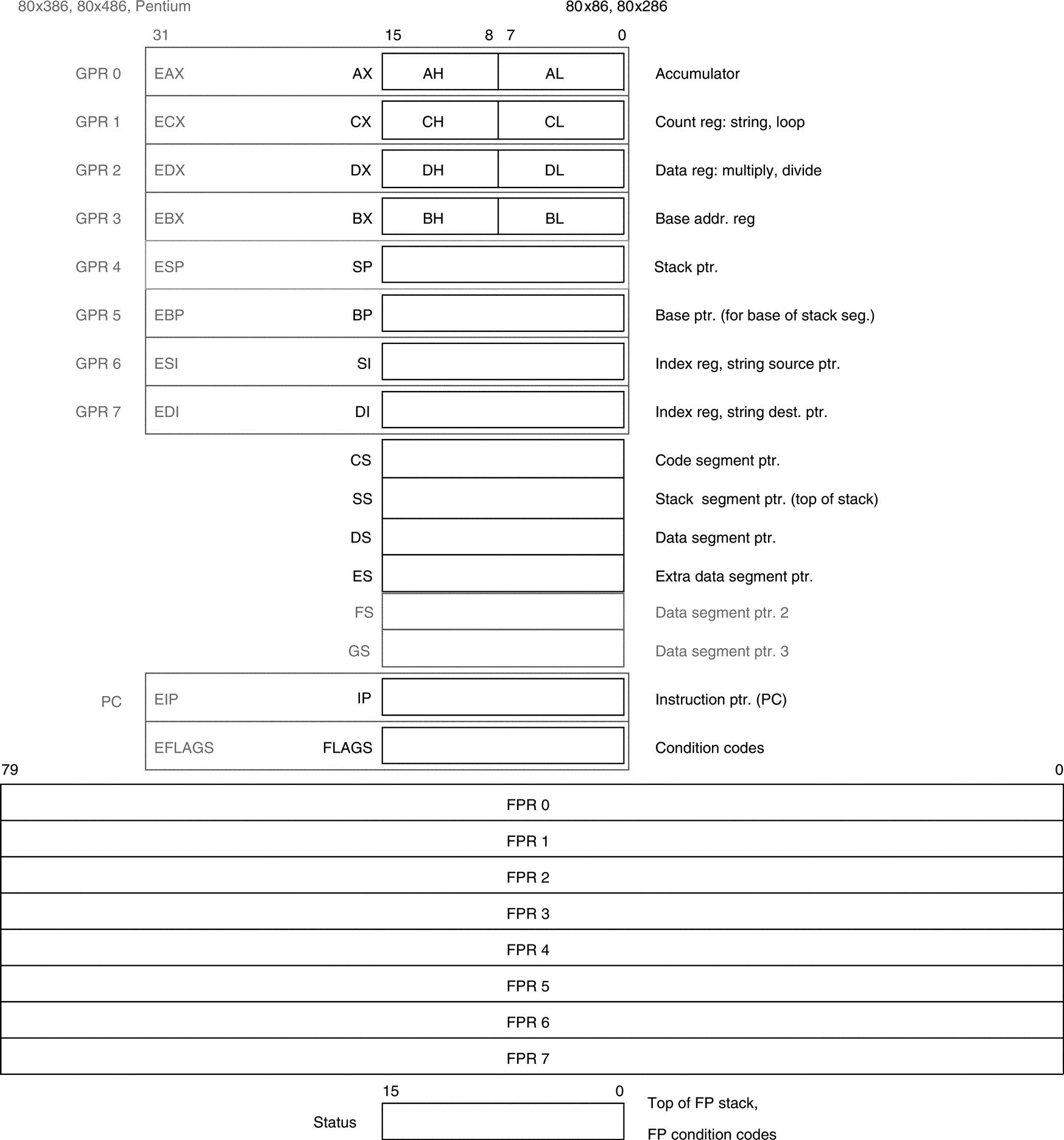
The original set is shown in black and the extended set in gray. The 8086 divided the first four registers in half so that they could be used either as one 16-bit register or as two 8-bit registers. Starting with the 80386, the top eight registers were extended to 32 bits and could also be used as general-purpose registers. The floating-point registers on the bottom are 80 bits wide, and although they look like regular registers they are not. They implement a stack, with the top of stack pointed to by the status register. One operand must be the top of stack, and the other can be any of the other seven registers below the top of stack.
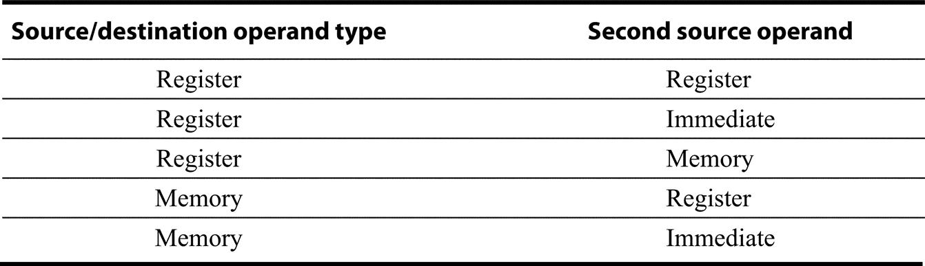
The 80x86 allows the combinations shown. The only restriction is the absence of a memory-memory mode. Immediates may be 8, 16, or 32 bits in length; a register is any one of the 14 major registers in Figure K.30 (not IP or FLAGS).
To explain the addressing modes, we need to keep in mind whether we are talking about the 16-bit mode used by both the 8086 and 80286 or the 32-bit mode available on the 80386 and its successors. The seven data memory addressing modes supported are
Displacements can be 8 or 32 bits in 32-bit mode, and 8 or 16 bits in 16-bit mode. If we count the size of the address as a separate addressing mode, the total is 11 addressing modes.
Although a memory operand can use any addressing mode, there are restrictions on what registers can be used in a mode. The section “80x86 Instruction Encoding” on page K-11 gives the full set of restrictions on registers, but the following description of addressing modes gives the basic register options:
- Absolute—With 16-bit or 32-bit displacement, depending on the mode.
- Register indirect—BX, SI, DI in 16-bit mode and EAX, ECX, EDX, EBX, ESI, and EDI in 32-bit mode.
- Based mode with 8-bit or 16-bit/32-bit displacement—BP, BX, SI, and DI in 16-bit mode and EAX, ECX, EDX, EBX, ESI, and EDI in 32-bit mode. The displacement is either 8 bits or the size of the address mode: 16 or 32 bits. (Intel gives two different names to this single addressing mode, based and indexed, but they are essentially identical and we combine them. This book uses indexed addressing to mean something different, explained next.)
- Indexed—The address is the sum of two registers. The allowable combinations are BX+SI, BX+DI, BP+SI, and BP+DI. This mode is called based indexed on the 8086. (The 32-bit mode uses a different addressing mode to get the same effect.)
- Based indexed with 8- or 16-bit displacement—The address is the sum of displacement and contents of two registers. The same restrictions on registers apply as in indexed mode.
- Base plus scaled indexed—This addressing mode and the next were added in the 80386 and are only available in 32-bit mode. The address calculation is

where Scale has the value 0, 1, 2, or 3; Index register can be any of the eight 32-bit general registers except ESP; and Base register can be any of the eight 32-bit general registers. - Base plus scaled index with 8- or 32-bit displacement—The address is the sum of the displacement and the address calculated by the scaled mode immediately above. The same restrictions on registers apply.
The 80x86 uses Little Endian addressing.
Ideally, we would refer discussion of 80x86 logical and physical addresses to Chapter 2, but the segmented address space prevents us from hiding that information. Figure K.32 shows the memory mapping options on the generations of 80x86 machines; Chapter 2 describes the segmented protection scheme in greater detail.
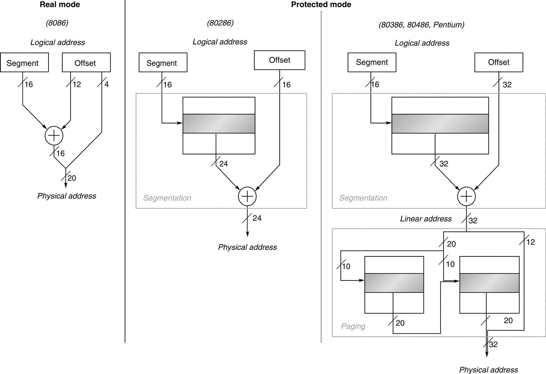
All 80x86 processors support this style of addressing, called real mode. It simply takes the contents of a segment register, shifts it left 4 bits, and adds it to the 16-bit offset, forming a 20-bit physical address. The 80286 (center) used the contents of the segment register to select a segment descriptor, which includes a 24-bit base address among other items. It is added to the 16-bit offset to form the 24-bit physical address. The 80386 and successors (right) expand this base address in the segment descriptor to 32 bits and also add an optional paging layer below segmentation. A 32-bit linear address is first formed from the segment and offset, and then this address is divided into two 10-bit fields and a 12-bit page offset. The first 10-bit field selects the entry in the first-level page table, and then this entry is used in combination with the second 10-bit field to access the second-level page table to select the upper 20 bits of the physical address. Prepending this 20-bit address to the final 12-bit field gives the 32-bit physical address. Paging can be turned off, redefining the 32-bit linear address as the physical address. Note that a “flat” 80x86 address space comes simply by loading the same value in all the segment registers; that is, it doesn’t matter which segment register is selected.
The assembly language programmer clearly must specify which segment register should be used with an address, no matter which address mode is used. To save space in the instructions, segment registers are selected automatically depending on which address register is used. The rules are simple: References to instructions (IP) use the code segment register (CS), references to the stack (BP or SP) use the stack segment register (SS), and the default segment register for the other registers is the data segment register (DS). The next section explains how they can be overridden.
80x86 Integer Operations
The 8086 provides support for both 8-bit (byte) and 16-bit (called word) data types. The data type distinctions apply to register operations as well as memory accesses. The 80386 adds 32-bit addresses and data, called double words. Almost every operation works on both 8-bit data and one longer data size. That size is determined by the mode and is either 16 or 32 bits.
Clearly some programs want to operate on data of all three sizes, so the 80x86 architects provide a convenient way to specify each version without expanding code size significantly. They decided that most programs would be dominated by either 16- or 32-bit data, and so it made sense to be able to set a default large size. This default size is set by a bit in the code segment register. To override the default size, an 8-bit prefix is attached to the instruction to tell the machine to use the other large size for this instruction.
The prefix solution was borrowed from the 8086, which allows multiple prefixes to modify instruction behavior. The three original prefixes override the default segment register, lock the bus so as to perform a semaphore (see Chapter 5), or repeat the following instruction until CX counts down to zero. This last prefix was intended to be paired with a byte move instruction to move a variable number of bytes. The 80386 also added a prefix to override the default address size.
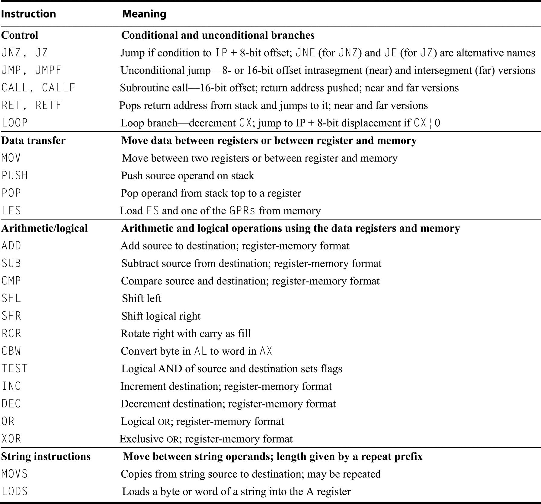
The 80x86 integer operations can be divided into four major classes:
- 1. Data movement instructions, including move, push, and pop
- 2. Arithmetic and logic instructions, including logical operations, test, shifts, and integer and decimal arithmetic operations
- 3. Control flow, including conditional branches and unconditional jumps, calls, and returns
- 4. String instructions, including string move and string compare
Figure K.33 shows some typical 80x86 instructions and their functions.
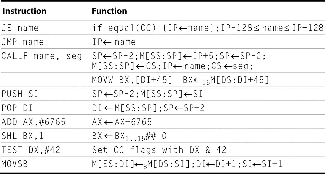
A list of frequent operations appears in Figure K.34. We use the abbreviation SR:X to indicate the formation of an address with segment register SR and offset X. This effective address corresponding to SR:X is (SR<<4)+X. The CALLF saves the IP of the next instruction and the current CS on the stack.
The data transfer, arithmetic, and logic instructions are unremarkable, except that the arithmetic and logic instruction operations allow the destination to be either a register or a memory location.
Control flow instructions must be able to address destinations in another segment. This is handled by having two types of control flow instructions: “near” for intrasegment (within a segment) and “far” for intersegment (between segments) transfers. In far jumps, which must be unconditional, two 16-bit quantities follow the opcode in 16-bit mode. One of these is used as the instruction pointer, while the other is loaded into CS and becomes the new code segment. In 32-bit mode the first field is expanded to 32 bits to match the 32-bit program counter (EIP).
Calls and returns work similarly—a far call pushes the return instruction pointer and return segment on the stack and loads both the instruction pointer and the code segment. A far return pops both the instruction pointer and the code segment from the stack. Programmers or compiler writers must be sure to always use the same type of call and return for a procedure—a near return does not work with a far call, and vice versa.
String instructions are part of the 8080 ancestry of the 80x86 and are not commonly executed in most programs.
Figure K.34 lists some of the integer 80x86 instructions. Many of the instructions are available in both byte and word formats.
80x86 Floating-Point Operations
Intel provided a stack architecture with its floating-point instructions: loads push numbers onto the stack, operations find operands in the top two elements of the stacks, and stores can pop elements off the stack, just as the stack example in Figure A.31 on page A-4 suggests.
Intel supplemented this stack architecture with instructions and addressing modes that allow the architecture to have some of the benefits of a register-memory model. In addition to finding operands in the top two elements of the stack, one operand can be in memory or in one of the seven registers below the top of the stack.
This hybrid is still a restricted register-memory model, however, in that loads always move data to the top of the stack while incrementing the top of stack pointer and stores can only move the top of stack to memory. Intel uses the notation ST to indicate the top of stack, and ST(i) to represent the ith register below the top of stack.
One novel feature of this architecture is that the operands are wider in the register stack than they are stored in memory, and all operations are performed at this wide internal precision. Numbers are automatically converted to the internal 80-bit format on a load and converted back to the appropriate size on a store. Memory data can be 32-bit (single-precision) or 64-bit (double-precision) floating-point numbers, called real by Intel. The register-memory version of these instructions will then convert the memory operand to this Intel 80-bit format before performing the operation. The data transfer instructions also will automatically convert 16- and 32-bit integers to reals, and vice versa, for integer loads and stores.
The 80x86 floating-point operations can be divided into four major classes:
- 1. Data movement instructions, including load, load constant, and store
- 2. Arithmetic instructions, including add, subtract, multiply, divide, square root, and absolute value
- 3. Comparison, including instructions to send the result to the integer CPU so that it can branch
- 4. Transcendental instructions, including sine, cosine, log, and exponentiation
Figure K.35 shows some of the 60 floating-point operations. We use the curly brackets {} to show optional variations of the basic operations: {I} means there is an integer version of the instruction, {P} means this variation will pop one operand off the stack after the operation, and {R} means reverse the sense of the operands in this operation.
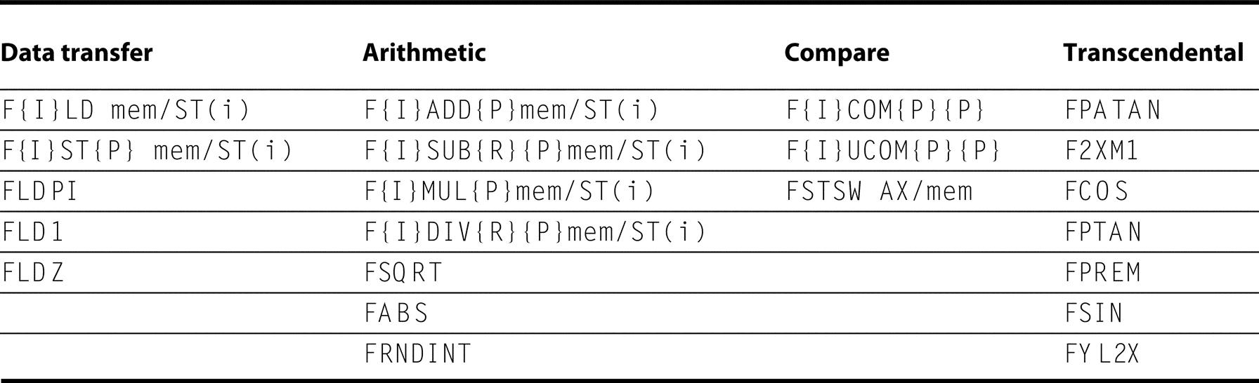
The first column shows the data transfer instructions, which move data to memory or to one of the registers below the top of the stack. The last three operations push constants on the stack: pi, 1.0, and 0.0. The second column contains the arithmetic operations described above. Note that the last three operate only on the top of stack. The third column is the compare instructions. Since there are no special floating-point branch instructions, the result of the compare must be transferred to the integer CPU via the FSTSW instruction, either into the AX register or into memory, followed by an SAHF instruction to set the condition codes. The floating-point comparison can then be tested using integer branch instructions. The final column gives the higher-level floating-point operations.
Not all combinations are provided. Hence,
F{I}SUB{R}{P}
represents these instructions found in the 80x86:
FSUB
FISUB
FSUBR
FISUBR
FSUBP
FSUBRP
There are no pop or reverse pop versions of the integer subtract instructions.
Note that we get even more combinations when including the operand modes for these operations. The floating-point add has these options, ignoring the integer and pop versions of the instruction:
| FADD | Both operands are in the in stack, and the result replaces the top of stack. |
| FADD ST(i) | One source operand is ith register below the top of stack, and the result replaces the top of stack. |
| FADD ST(i),ST | One source operand is the top of stack, and the result replaces ith register below the top of stack. |
| FADD mem32 | One source operand is a 32-bit location in memory, and the result replaces the top of stack. |
| FADD mem64 | One source operand is a 64-bit location in memory, and the result replaces the top of stack. |
As mentioned earlier SSE2 presents a model of IEEE floating-point registers.
80x86 Instruction Encoding
Saving the worst for last, the encoding of instructions in the 8086 is complex, with many different instruction formats. Instructions may vary from 1 byte, when there are no operands, to up to 6 bytes, when the instruction contains a 16-bit immediate and uses 16-bit displacement addressing. Prefix instructions increase 8086 instruction length beyond the obvious sizes.
The 80386 additions expand the instruction size even further, as Figure K.36 shows. Both the displacement and immediate fields can be 32 bits long, two more prefixes are possible, the opcode can be 16 bits long, and the scaled index mode specifier adds another 8 bits. The maximum possible 80386 instruction is 17 bytes long.
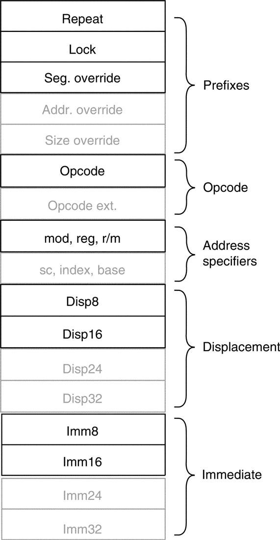
Every field is optional except the opcode.
Figure K.37 shows the instruction format for several of the example instructions in Figure K.33. The opcode byte usually contains a bit saying whether the operand is a byte wide or the larger size, 16 bits or 32 bits depending on the mode. For some instructions, the opcode may include the addressing mode and the register; this is true in many instructions that have the form register ← register op immediate. Other instructions use a “postbyte” or extra opcode byte, labeled “mod, reg, r/m” in Figure K.36, which contains the addressing mode information. This postbyte is used for many of the instructions that address memory. The based with scaled index uses a second postbyte, labeled “sc, index, base” in Figure K.36.

Many instructions contain the 1-bit field w, which says whether the operation is a byte or a word. Fields of the form v/w or d/w are a d-field or v-field followed by the w-field. The d-field in MOV is used in instructions that may move to or from memory and shows the direction of the move. The field v in the SHL instruction indicates a variable-length shift; variable-length shifts use a register to hold the shift count. The ADD instruction shows a typical optimized short encoding usable only when the first operand is AX. Overall instructions may vary from 1 to 6 bytes in length.
The floating-point instructions are encoded in the escape opcode of the 8086 and the postbyte address specifier. The memory operations reserve 2 bits to decide whether the operand is a 32- or 64-bit real or a 16- or 32-bit integer. Those same 2 bits are used in versions that do not access memory to decide whether the stack should be popped after the operation and whether the top of stack or a lower register should get the result.
Alas, you cannot separate the restrictions on registers from the encoding of the addressing modes in the 80x86. Hence, Figures K.38 and K.39 show the encoding of the two postbyte address specifiers for both 16- and 32-bit mode.
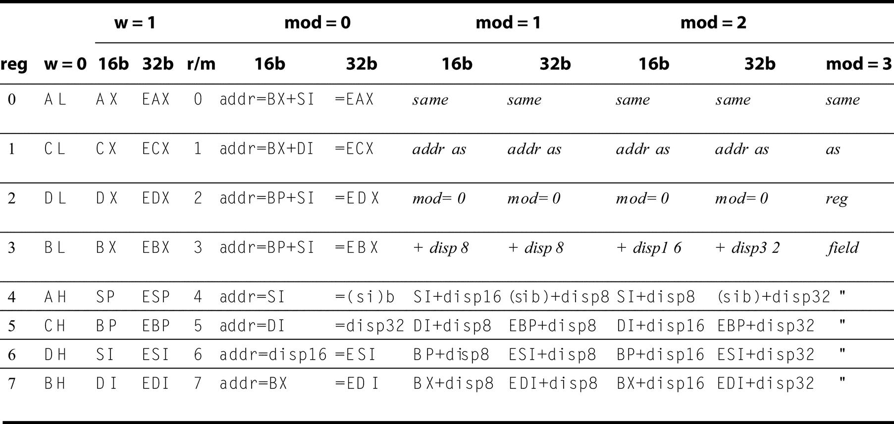
The first four columns show the encoding of the 3-bit reg field, which depends on the w bit from the opcode and whether the machine is in 16- or 32-bit mode. The remaining columns explain the mod and r/m fields. The meaning of the 3-bit r/m field depends on the value in the 2-bit mod field and the address size. Basically, the registers used in the address calculation are listed in the sixth and seventh columns, under mod = 0, with mod = 1 adding an 8-bit displacement and mod = 2 adding a 16- or 32-bit displacement, depending on the address mode. The exceptions are r/m = 6 when mod = 1 or mod = 2 in 16-bit mode selects BP plus the displacement; r/m = 5 when mod = 1 or mod = 2 in 32-bit mode selects EBP plus displacement; and r/m = 4 in 32-bit mode when mod ¦3 (sib) means use the scaled index mode shown in Figure K.39. When mod = 3, the r/m field indicates a register, using the same encoding as the reg field combined with the w bit.
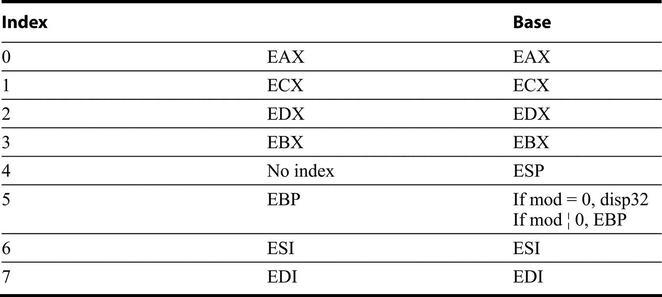
This mode is indicated by the (sib) notation in Figure K.38. Note that this mode expands the list of registers to be used in other modes: Register indirect using ESP comes from Scale = 0, Index = 4, and Base = 4, and base displacement with EBP comes from Scale = 0, Index = 5, and mod = 0. The two-bit scale field is used in this formula of the effective address: Base register + 2Scale × Index register.
Putting It All Together: Measurements of Instruction Set Usage
In this section, we present detailed measurements for the 80x86 and then compare the measurements to MIPS for the same programs. To facilitate comparisons among dynamic instruction set measurements, we use a subset of the SPEC92 programs. The 80x86 results were taken in 1994 using the Sun Solaris FORTRAN and C compilers V2.0 and executed in 32-bit mode. These compilers were comparable in quality to the compilers used for MIPS.
Remember that these measurements depend on the benchmarks chosen and the compiler technology used. Although we feel that the measurements in this section are reasonably indicative of the usage of these architectures, other programs may behave differently from any of the benchmarks here, and different compilers may yield different results. In doing a real instruction set study, the architect would want to have a much larger set of benchmarks, spanning as wide an application range as possible, and consider the operating system and its usage of the instruction set. Single-user benchmarks like those measured here do not necessarily behave in the same fashion as the operating system.
We start with an evaluation of the features of the 80x86 in isolation, and later compare instruction counts with those of DLX.
Measurements of 80x86 Operand Addressing
We start with addressing modes. Figure K.40 shows the distribution of the operand types in the 80x86. These measurements cover the “second” operand of the operation; for example,
mov EAX, [45]
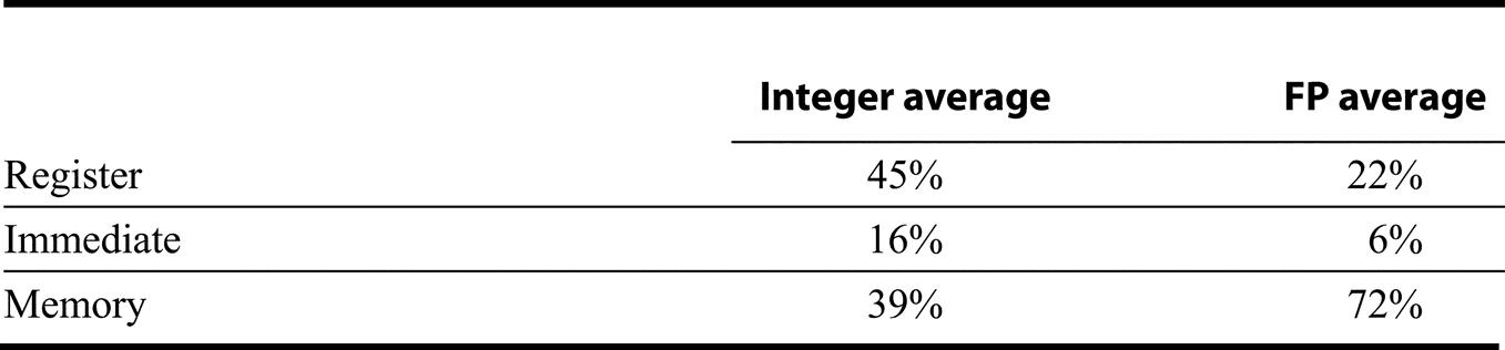
counts as a single memory operand. If the types of the first operand were counted, the percentage of register usage would increase by about a factor of 1.5.
The 80x86 memory operands are divided into their respective addressing modes in Figure K.41. Probably the biggest surprise is the popularity of the addressing modes added by the 80386, the last four rows of the figure. They account for about half of all the memory accesses. Another surprise is the popularity of direct addressing. On most other machines, the equivalent of the direct addressing mode is rare. Perhaps the segmented address space of the 80x86 makes direct addressing more useful, since the address is relative to a base address from the segment register.
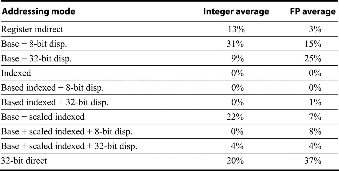
This chart does not include addressing modes used by branches or control instructions.
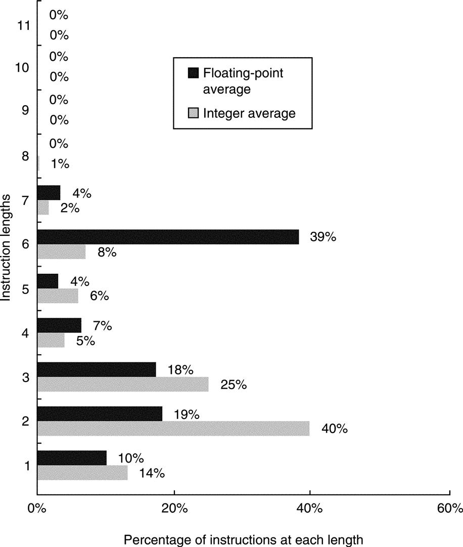
These addressing modes largely determine the size of the Intel instructions. Figure K.42 shows the distribution of instruction sizes. The average number of bytes per instruction for integer programs is 2.8, with a standard deviation of 1.5, and 4.1 with a standard deviation of 1.9 for floating-point programs. The difference in length arises partly from the differences in the addressing modes: Integer programs rely more on the shorter register indirect and 8-bit displacement addressing modes, while floating-point programs more frequently use the 80386 addressing modes with the longer 32-bit displacements.
Given that the floating-point instructions have aspects of both stacks and registers, how are they used? Figure K.43 shows that, at least for the compilers used in this measurement, the stack model of execution is rarely followed. (See Section L.3 for a historical explanation of this observation.)
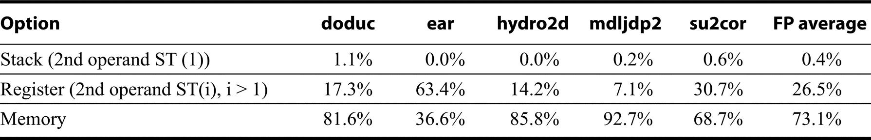
The three options are (1) the strict stack model of implicit operands on the stack, (2) register version naming an explicit operand that is not one of the top two elements of the stack, and (3) memory operand.
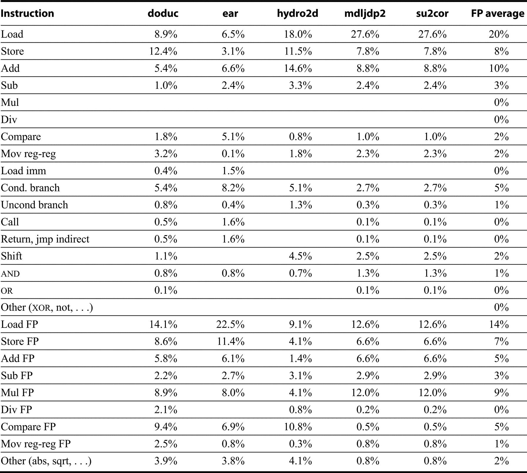
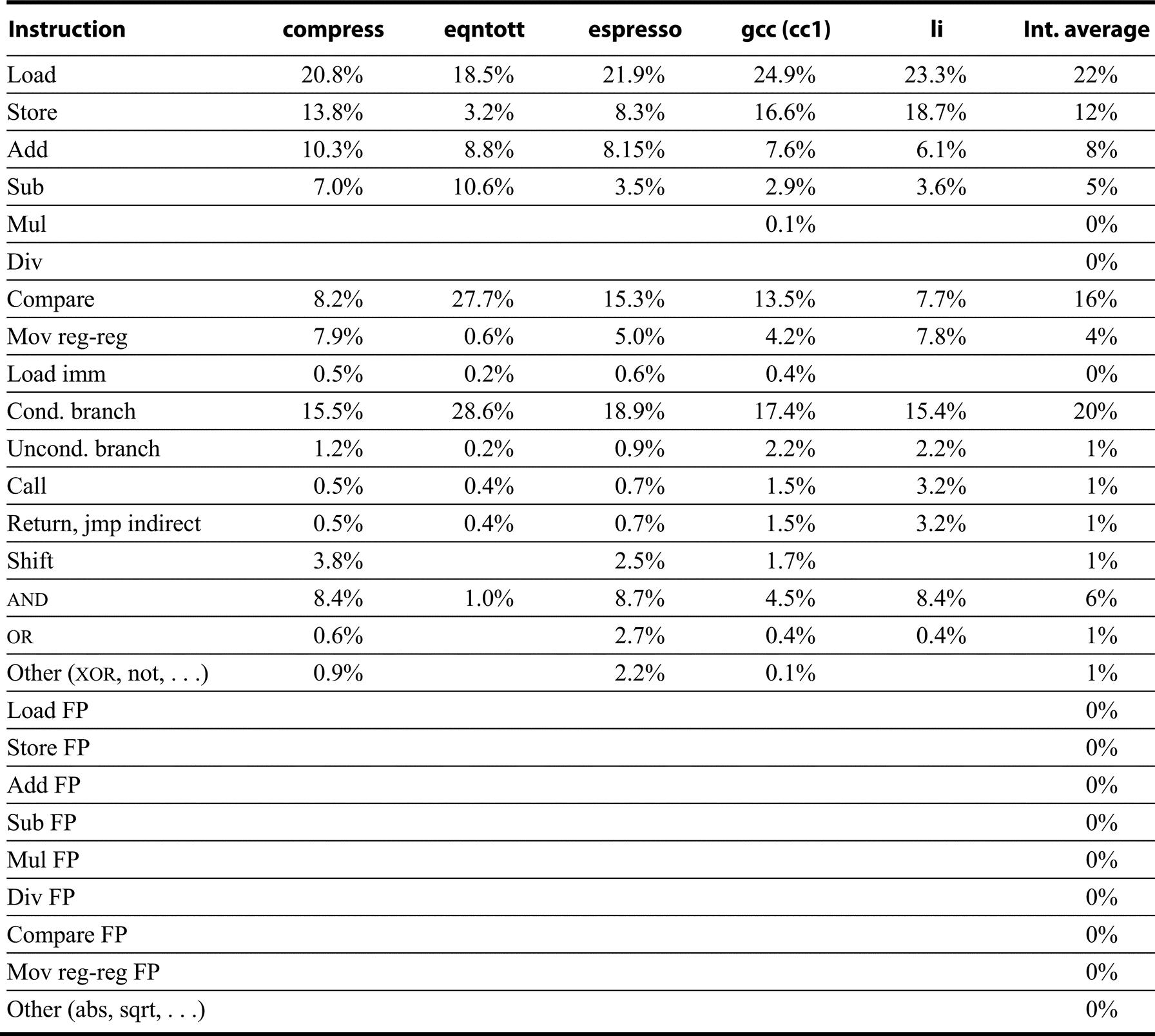
Finally, Figures K.44 and K.45 show the instruction mixes for 10 SPEC92 programs.
Comparative Operation Measurements
Figures K.46 and K.47 show the number of instructions executed for each of the 10 programs on the 80x86 and the ratio of instruction execution compared with that for DLX: Numbers less than 1.0 mean that the 80x86 executes fewer instructions than DLX. The instruction count is surprisingly close to DLX for many integer programs, as you would expect a load-store instruction set architecture like DLX to execute more instructions than a register-memory architecture like the 80x86. The floating-point programs always have higher counts for the 80x86, presumably due to the lack of floating-point registers and the use of a stack architecture.
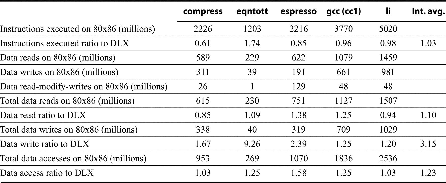
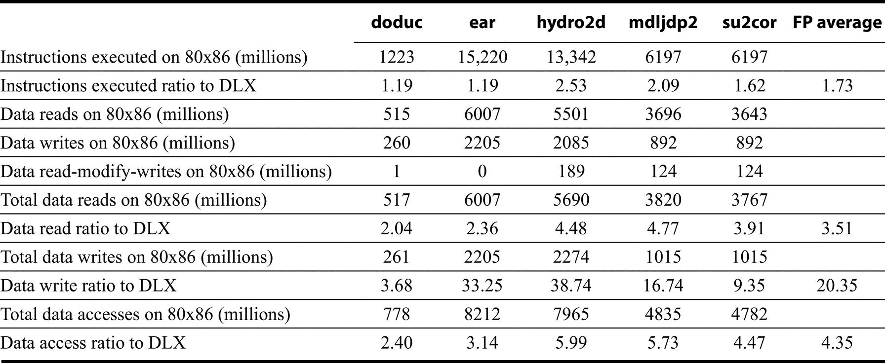
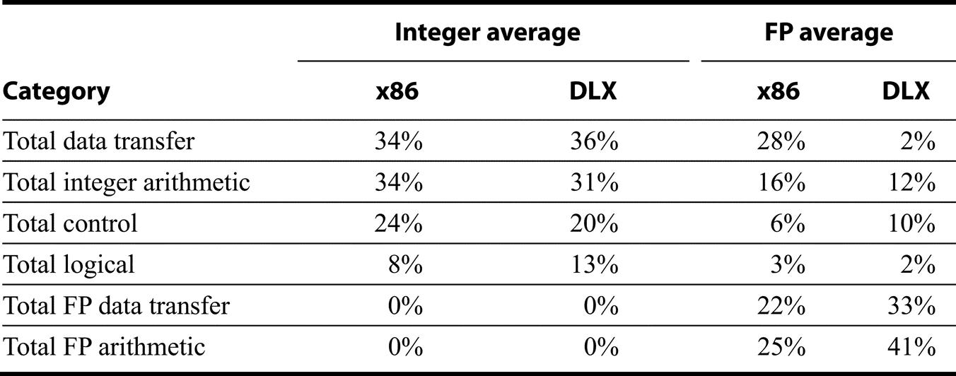
Another question is the total amount of data traffic for the 80x86 versus DLX, since the 80x86 can specify memory operands as part of operations while DLX can only access via loads and stores. Figures K.46 and K.47 also show the data reads, data writes, and data read-modify-writes for these 10 programs. The total accesses ratio to DLX of each memory access type is shown in the bottom rows, with the read-modify-write counting as one read and one write. The 80x86 performs about two to four times as many data accesses as DLX for floating-point programs, and 1.25 times as many for integer programs. Finally, Figure K.48 shows the percentage of instructions in each category for 80x86 and DLX.
Concluding Remarks
Beauty is in the eye of the beholder.
Old Adage
As we have seen, “orthogonal” is not a term found in the Intel architectural dictionary. To fully understand which registers and which addressing modes are available, you need to see the encoding of all addressing modes and sometimes the encoding of the instructions.
Some argue that the inelegance of the 80x86 instruction set is unavoidable, the price that must be paid for rampant success by any architecture. We reject that notion. Obviously, no successful architecture can jettison features that were added in previous implementations, and over time some features may be seen as undesirable. The awkwardness of the 80x86 began at its core with the 8086 instruction set and was exacerbated by the architecturally inconsistent expansions of the 8087, 80286, and 80386.
A counterexample is the IBM 360/370 architecture, which is much older than the 80x86. It dominates the mainframe market just as the 80x86 dominates the PC market. Due undoubtedly to a better base and more compatible enhancements, this instruction set makes much more sense than the 80x86 more than 30 years after its first implementation.
For better or worse, Intel had a 16-bit microprocessor years before its competitors’ more elegant architectures, and this head start led to the selection of the 8086 as the CPU for the IBM PC. What it lacks in style is made up in quantity, making the 80x86 beautiful from the right perspective.
The saving grace of the 80x86 is that its architectural components are not too difficult to implement, as Intel has demonstrated by rapidly improving performance of integer programs since 1978. High floating-point performance is a larger challenge in this architecture.
K.4 The VAX Architecture
VAX: the most successful minicomputer design in industry history . . . the VAX was probably the hacker’s favorite machine . . . . Especially noted for its large, assembler-programmer-friendly instruction set—an asset that became a liability after the RISC revolution.
Eric Raymond
The New Hacker’s Dictionary (1991)
Introduction
To enhance your understanding of instruction set architectures, we chose the VAX as the representative Complex Instruction Set Computer (CISC) because it is so different from MIPS and yet still easy to understand. By seeing two such divergent styles, we are confident that you will be able to learn other instruction sets on your own.
At the time the VAX was designed, the prevailing philosophy was to create instruction sets that were close to programming languages in order to simplify compilers. For example, because programming languages had loops, instruction sets should have loop instructions. As VAX architect William Strecker said (“VAX-11/780—A Virtual Address Extension to the PDP-11 Family,” AFIPS Proc., National Computer Conference, 1978):
A major goal of the VAX-11 instruction set was to provide for effective compiler generated code. Four decisions helped to realize this goal: 1) A very regular and consistent treatment of operators . . . . 2) An avoidance of instructions unlikely to be generated by a compiler . . . . 3) Inclusions of several forms of common operators . . . . 4) Replacement of common instruction sequences with single instructions . . . . Examples include procedure calling, multiway branching, loop control, and array subscript calculation.
Recall that DRAMs of the mid-1970s contained less than 1/1000th the capacity of today’s DRAMs, so code space was also critical. Hence, another prevailing philosophy was to minimize code size, which is de-emphasized in fixed-length instruction sets like MIPS. For example, MIPS address fields always use 16 bits, even when the address is very small. In contrast, the VAX allows instructions to be a variable number of bytes, so there is little wasted space in address fields.
Whole books have been written just about the VAX, so this VAX extension cannot be exhaustive. Hence, the following sections describe only a few of its addressing modes and instructions. To show the VAX instructions in action, later sections show VAX assembly code for two C procedures. The general style will be to contrast these instructions with the MIPS code that you are already familiar with.
The differing goals for VAX and MIPS have led to very different architectures. The VAX goals, simple compilers and code density, led to the powerful addressing modes, powerful instructions, and efficient instruction encoding. The MIPS goals were high performance via pipelining, ease of hardware implementation, and compatibility with highly optimizing compilers. The MIPS goals led to simple instructions, simple addressing modes, fixed-length instruction formats, and a large number of registers.
VAX Operands and Addressing Modes
The VAX is a 32-bit architecture, with 32-bit-wide addresses and 32-bit-wide registers. Yet, the VAX supports many other data sizes and types, as Figure K.49 shows. Unfortunately, VAX uses the name “word” to refer to 16-bit quantities; in this text, a word means 32 bits. Figure K.49 shows the conversion between the MIPS data type names and the VAX names. Be careful when reading about VAX instructions, as they refer to the names of the VAX data types.
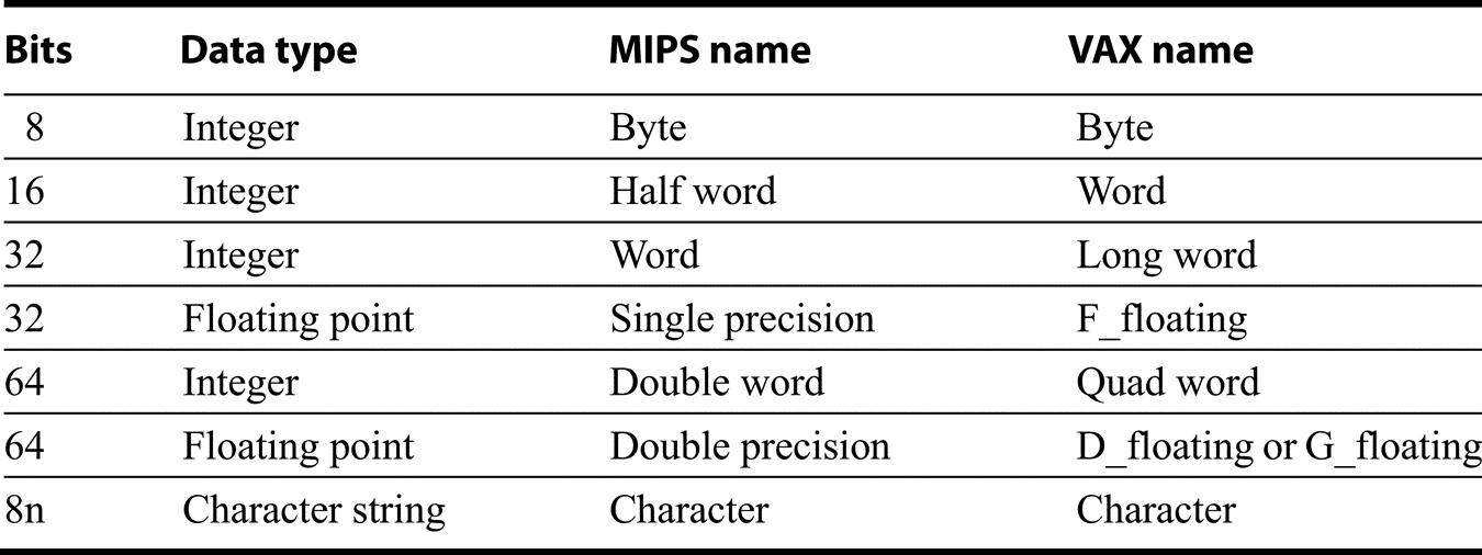
The first letter of the VAX type (b, w, l, f, q, d, g, c) is often used to complete an instruction name. Examples of move instructions include movb, movw, movl, movf, movq, movd, movg, and movc3. Each move instruction transfers an operand of the data type indicated by the letter following mov.
The VAX provides sixteen 32-bit registers. The VAX assembler uses the notation r0, r1, . . . , r15 to refer to these registers, and we will stick to that notation. Alas, 4 of these 16 registers are effectively claimed by the instruction set architecture. For example, r14 is the stack pointer (sp) and r15 is the program counter (pc). Hence, r15 cannot be used as a general-purpose register, and using r14 is very difficult because it interferes with instructions that manipulate the stack. The other dedicated registers are r12, used as the argument pointer (ap), and r13, used as the frame pointer (fp); their purpose will become clear later. (Like MIPS, the VAX assembler accepts either the register number or the register name.)
VAX addressing modes include those discussed in Appendix A, which has all the MIPS addressing modes: register, displacement, immediate, and PC-relative. Moreover, all these modes can be used for jump addresses or for data addresses.
But that’s not all the addressing modes. To reduce code size, the VAX has three lengths of addresses for displacement addressing: 8-bit, 16-bit, and 32-bit addresses called, respectively, byte displacement, word displacement, and long displacement addressing. Thus, an address can be not only as small as possible but also as large as necessary; large addresses need not be split, so there is no equivalent to the MIPS lui instruction (see Figure A.24 on page A-37).
Those are still not all the VAX addressing modes. Several have a deferred option, meaning that the object addressed is only the address of the real object, requiring another memory access to get the operand. This addressing mode is called indirect addressing in other machines. Thus, register deferred, autoincrement deferred, and byte/word/long displacement deferred are other addressing modes to choose from. For example, using the notation of the VAX assembler, r1 means the operand is register 1 and (r1) means the operand is the location in memory pointed to by r1.
There is yet another addressing mode. Indexed addressing automatically converts the value in an index operand to the proper byte address to add to the rest of the address. For a 32-bit word, we needed to multiply the index of a 4-byte quantity by 4 before adding it to a base address. Indexed addressing, called scaled addressing on some computers, automatically multiplies the index of a 4-byte quantity by 4 as part of the address calculation.
To cope with such a plethora of addressing options, the VAX architecture separates the specification of the addressing mode from the specification of the operation. Hence, the opcode supplies the operation and the number of operands, and each operand has its own addressing mode specifier. Figure K.50 shows the name, assembler notation, example, meaning, and length of the address specifier.
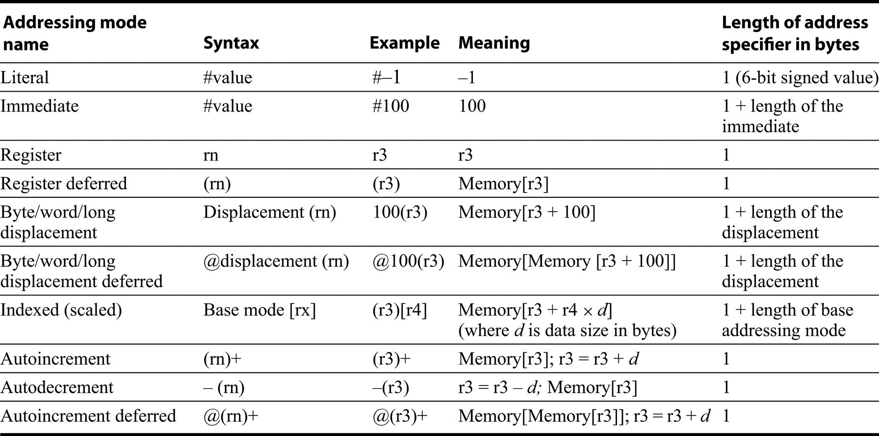
The length of each addressing mode is 1 byte plus the length of any displacement or immediate field needed by the mode. Literal mode uses a special 2-bit tag and the remaining 6 bits encode the constant value. If the constant is too big, it must use the immediate addressing mode. Note that the length of an immediate operand is dictated by the length of the data type indicated in the opcode, not the value of the immediate. The symbol d in the last four modes represents the length of the data in bytes; d is 4 for 32-bit add.
The VAX style of addressing means that an operation doesn’t know where its operands come from; a VAX add instruction can have three operands in registers, three operands in memory, or any combination of registers and memory operands.
In this example instruction, we show the VAX destination operand on the left and the source operands on the right, just as we show MIPS code. The VAX assembler actually expects operands in the opposite order, but we felt it would be less confusing to keep the destination on the left for both machines. Obviously, left or right orientation is arbitrary; the only requirement is consistency.
- Elaboration Because the PC is 1 of the 16 registers that can be selected in a VAX addressing mode, 4 of the 22 VAX addressing modes are synthesized from other addressing modes. Using the PC as the chosen register in each case, immediate addressing is really autoincrement, PC-relative is displacement, absolute is autoincrement deferred, and relative deferred is displacement deferred.
Encoding VAX Instructions
Given the independence of the operations and addressing modes, the encoding of instructions is quite different from MIPS.
VAX instructions begin with a single byte opcode containing the operation and the number of operands. The operands follow the opcode. Each operand begins with a single byte, called the address specifier, that describes the addressing mode for that operand. For a simple addressing mode, such as register addressing, this byte specifies the register number as well as the mode (see the rightmost column in Figure K.50). In other cases, this initial byte can be followed by many more bytes to specify the rest of the address information.
As a specific example, let’s show the encoding of the add instruction from the example on page K-24:
addl3 r1,737(r2),(r3)[r4]
Assume that this instruction starts at location 201.
Figure K.51 shows the encoding. Note that the operands are stored in memory in opposite order to the assembly code above. The execution of VAX instructions begins with fetching the source operands, so it makes sense for them to come first. Order is not important in fixed-length instructions like MIPS, since the source and destination operands are easily found within a 32-bit word.
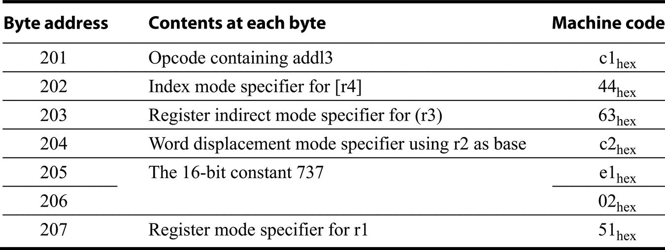
To satisfy your curiosity, the right column shows the actual VAX encoding in hexadecimal notation. Note that the 16-bit constant 737ten takes 2 bytes.
The first byte, at location 201, is the opcode. The next byte, at location 202, is a specifier for the index mode using register r4. Like many of the other specifiers, the left 4 bits of the specifier give the mode and the right 4 bits give the register used in that mode. Since addl3 is a 4-byte operation, r4 will be multiplied by 4 and added to whatever address is specified next. In this case it is register deferred addressing using register r3. Thus, bytes 202 and 203 combined define the third operand in the assembly code.
The following byte, at address 204, is a specifier for word displacement addressing using register r2 as the base register. This specifier tells the VAX that the following two bytes, locations 205 and 206, contain a 16-bit address to be added to r2.
The final byte of the instruction gives the destination operand, and this specifier selects register addressing using register r1.
Such variability in addressing means that a single VAX operation can have many different lengths; for example, an integer add varies from 3 bytes to 19 bytes. VAX implementations must decode the first operand before they can find the second, and so implementors are strongly tempted to take 1 clock cycle to decode each operand; thus, this sophisticated instruction set architecture can result in higher clock cycles per instruction, even when using simple addresses.
VAX Operations
In keeping with its philosophy, the VAX has a large number of operations as well as a large number of addressing modes. We review a few here to give the flavor of the machine.
Given the power of the addressing modes, the VAX move instruction performs several operations found in other machines. It transfers data between any two addressable locations and subsumes load, store, register-register moves, and memory-memory moves as special cases. The first letter of the VAX data type (b, w, l, f, q, d, g, c in Figure K.49) is appended to the acronym mov to determine the size of the data. One special move, called move address, moves the 32-bit address of the operand rather than the data. It uses the acronym mova.
The arithmetic operations of MIPS are also found in the VAX, with two major differences. First, the type of the data is attached to the name. Thus, addb, addw, and addl operate on 8-bit, 16-bit, and 32-bit data in memory or registers, respectively; MIPS has a single add instruction that operates only on the full 32-bit register. The second difference is that to reduce code size the add instruction specifies the number of unique operands; MIPS always specifies three even if one operand is redundant. For example, the MIPS instruction
add $1, $1, $2
takes 32 bits like all MIPS instructions, but the VAX instruction
addl2 r1, r2
uses r1 for both the destination and a source, taking just 24 bits: 8 bits for the opcode and 8 bits each for the two register specifiers.
Number of Operations
Now we can show how VAX instruction names are formed:
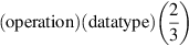
The operation add works with data types byte, word, long, float, and double and comes in versions for either 2 or 3 unique operands, so the following instructions are all found in the VAX:
addb2     addw2     addl2     addf2     addd2
addb3     addw3     addl3     addf3     addd3
Accounting for all addressing modes (but ignoring register numbers and immediate values) and limiting to just byte, word, and long, there are more than 30,000 versions of integer add in the VAX; MIPS has just 4!
Another reason for the large number of VAX instructions is the instructions that either replace sequences of instructions or take fewer bytes to represent a single instruction. Here are four such examples (* means the data type):
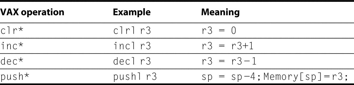
The push instruction in the last row is exactly the same as using the move instruction with autodecrement addressing on the stack pointer:
movl – (sp), r3
Brevity is the advantage of pushl: It is 1 byte shorter since sp is implied.
Branches, Jumps, and Procedure Calls
The VAX branch instructions are related to the arithmetic instructions because the branch instructions rely on condition codes. Condition codes are set as a side effect of an operation, and they indicate whether the result is positive, negative, or zero or if an overflow occurred. Most instructions set the VAX condition codes according to their result; instructions without results, such as branches, do not. The VAX condition codes are N (Negative), Z (Zero), V (oVerflow), and C (Carry). There is also a compare instruction cmp* just to set the condition codes for a subsequent branch.
The VAX branch instructions include all conditions. Popular branch instructions include beql(=), bneq(≠), blss(<), bleq(≤), bgtr(>), and bgeq(≥), which do just what you would expect. There are also unconditional branches whose name is determined by the size of the PC-relative offset. Thus, brb (branch byte) has an 8-bit displacement, and brw (branch word) has a 16-bit displacement.
The final major category we cover here is the procedure call and return instructions. Unlike the MIPS architecture, these elaborate instructions can take dozens of clock cycles to execute. The next two sections show how they work, but we need to explain the purpose of the pointers associated with the stack manipulated by calls and ret. The stack pointer, sp, is just like the stack pointer in MIPS; it points to the top of the stack. The argument pointer, ap, points to the base of the list of arguments or parameters in memory that are passed to the procedure. The frame pointer, fp, points to the base of the local variables of the procedure that are kept in memory (the stack frame). The VAX call and return instructions manipulate these pointers to maintain the stack in proper condition across procedure calls and to provide convenient base registers to use when accessing memory operands. As we shall see, call and return also save and restore the general-purpose registers as well as the program counter. Figure K.52 gives a further sampling of the VAX instruction set.
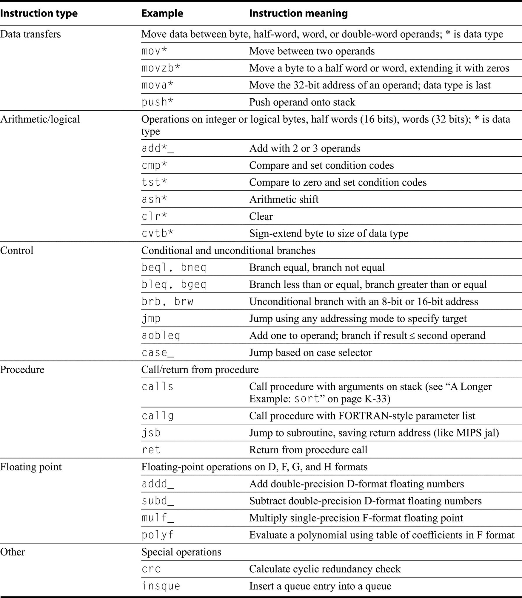
An Example to Put It All Together: swap
To see programming in VAX assembly language, we translate two C procedures, swap and sort. The C code for swap is reproduced in Figure K.53. The next section covers sort.
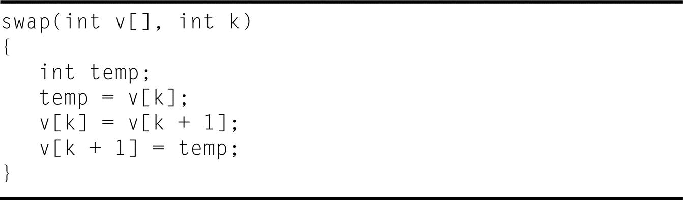
This procedure will be used in the sorting example in the next section.
We describe the swap procedure in three general steps of assembly language programming:
The VAX code for these procedures is based on code produced by the VMS C compiler using optimization.
Register Allocation for swap
In contrast to MIPS, VAX parameters are normally allocated to memory, so this step of assembly language programming is more properly called “variable allocation.” The standard VAX convention on parameter passing is to use the stack. The two parameters, v[] and k, can be accessed using register ap, the argument pointer: The address 4(ap) corresponds to v[] and 8(ap) corresponds to k. Remember that with byte addressing the address of sequential 4-byte words differs by 4. The only other variable is temp, which we associate with register r3.
Code for the Body of the Procedure swap
The remaining lines of C code in swap are
temp = v[k];
v[k] = v[k + 1];
v[k + 1] = temp;
Since this program uses v[] and k several times, to make the programs run faster the VAX compiler first moves both parameters into registers:
movl r2, 4(ap) ;r2 = v[]
movl r1, 8(ap) ;r1 = k
Note that we follow the VAX convention of using a semicolon to start a comment; the MIPS comment symbol # represents a constant operand in VAX assembly language.
The VAX has indexed addressing, so we can use index k without converting it to a byte address. The VAX code is then straightforward:
movl  r3, (r2)[r1]      ;r3 (temp) = v[k]
addl3 r0, #1,8(ap)      ;r0 = k + 1
movl (r2)[r1],(r2)[r0]  ;v[k] = v[r0] (v[k + 1])
movl (r2)[r0],r3        ;v[k + 1] = r3 (temp)
Unlike the MIPS code, which is basically two loads and two stores, the key VAX code is one memory-to-register move, one memory-to-memory move, and one register-to-memory move. Note that the addl3 instruction shows the flexibility of the VAX addressing modes: It adds the constant 1 to a memory operand and places the result in a register.
Now we have allocated storage and written the code to perform the operations of the procedure. The only missing item is the code that preserves registers across the routine that calls swap.
Preserving Registers across Procedure Invocation of swap
The VAX has a pair of instructions that preserve registers, calls and ret. This example shows how they work.
The VAX C compiler uses a form of callee convention. Examining the code above, we see that the values in registers r0, r1, r2, and r3 must be saved so that they can later be restored. The calls instruction expects a 16-bit mask at the beginning of the procedure to determine which registers are saved: if bit i is set in the mask, then register i is saved on the stack by the calls instruction. In addition, calls saves this mask on the stack to allow the return instruction (ret) to restore the proper registers. Thus, the calls executed by the caller does the saving, but the callee sets the call mask to indicate what should be saved.
One of the operands for calls gives the number of parameters being passed, so that calls can adjust the pointers associated with the stack: the argument pointer (ap), frame pointer (fp), and stack pointer (sp). Of course, calls also saves the program counter so that the procedure can return!
Thus, to preserve these four registers for swap, we just add the mask at the beginning of the procedure, letting the calls instruction in the caller do all the work:
.word ˆm<r0,r1,r2,r3 > ;set bits in mask for 0,1,2,3
This directive tells the assembler to place a 16-bit constant with the proper bits set to save registers r0 through r3.
The return instruction undoes the work of calls. When finished, ret sets the stack pointer from the current frame pointer to pop everything calls placed on the stack. Along the way, it restores the register values saved by calls, including those marked by the mask and old values of the fp, ap, and pc.
To complete the procedure swap, we just add one instruction:
ret ;restore registers and return
The Full Procedure swap
We are now ready for the whole routine. Figure K.54 identifies each block of code with its purpose in the procedure, with the MIPS code on the left and the VAX code on the right. This example shows the advantage of the scaled indexed addressing and the sophisticated call and return instructions of the VAX in reducing the number of lines of code. The 17 lines of MIPS assembly code became 8 lines of VAX assembly code. It also shows that passing parameters in memory results in extra memory accesses.
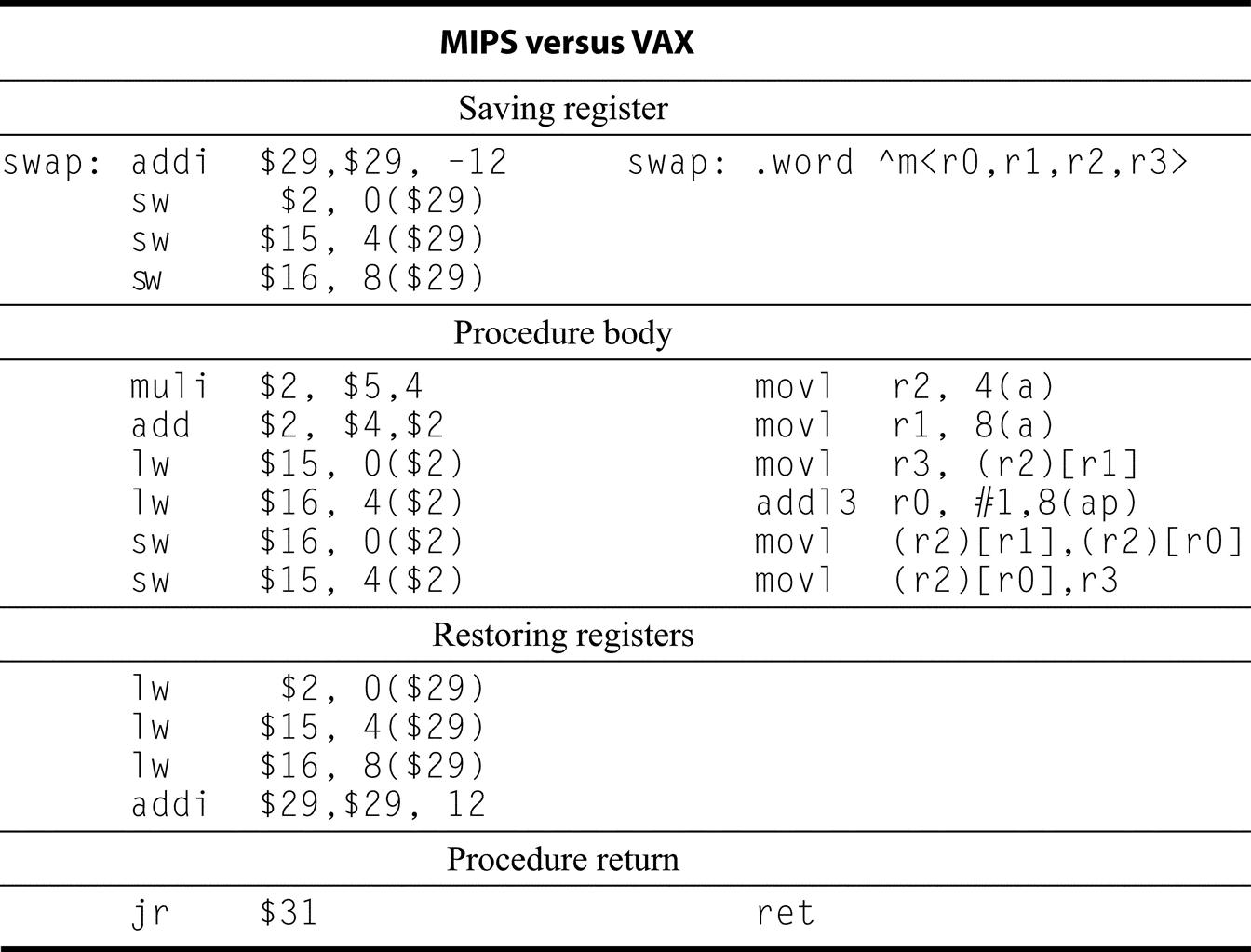
Keep in mind that the number of instructions executed is not the same as performance; the fallacy on page K-38 makes this point.
Note that VAX software follows a convention of treating registers r0 and r1 as temporaries that are not saved across a procedure call, so the VMS C compiler does include registers r0 and r1 in the register saving mask. Also, the C compiler should have used r1 instead of 8(ap) in the addl3 instruction; such examples inspire computer architects to try to write compilers!
A Longer Example: sort
We show the longer example of the sort procedure. Figure K.55 shows the C version of the program. Once again we present this procedure in several steps, concluding with a side-by-side comparison to MIPS code.

Register Allocation for sort
The two parameters of the procedure sort, v and n, are found in the stack in locations 4(ap) and 8(ap), respectively. The two local variables are assigned to registers: i to r6 and j to r4. Because the two parameters are referenced frequently in the code, the VMS C compiler copies the address of these parameters into registers upon entering the procedure:
moval  r7,8(ap)  ;move  address  of  n  into  r7
moval  r5,4(ap)  ;move  address  of  v  into  r5
It would seem that moving the value of the operand to a register would be more useful than its address, but once again we bow to the decision of the VMS C compiler. Apparently the compiler cannot be sure that v and n don’t overlap in memory.
Code for the Body of the sort Procedure
The procedure body consists of two nested for loops and a call to swap, which includes parameters. Let’s unwrap the code from the outside to the middle.
The Outer Loop
The first translation step is the first for loop:
for (i = 0; i < n; i = i + 1) {
Recall that the C for statement has three parts: initialization, loop test, and iteration increment. It takes just one instruction to initialize i to 0, the first part of the for statement:
clrl r6 ;i = 0
It also takes just one instruction to increment i, the last part of the for:
incl r6 ;i = i + 1
The loop should be exited if i < n is false, or said another way, exit the loop if i ≥ n. This test takes two instructions:
for1tst: cmpl r6,(r7) ;compare r6 and memory[r7] (i:n)
          bgeq exit1  ;go to exit1 if r6 ≥ mem[r7] (i ≥ n)
Note that cmpl sets the condition codes for use by the conditional branch instruction bgeq.
The bottom of the loop just jumps back to the loop test:
          brb  for1tst  ;branch to test of outer loop
exit1:
The skeleton code of the first for loop is then
          clrl  r6       ;i = 0
for1tst: cmpl  r6,(r7)   ;compare r6 and memory[r7] (i:n)
          bgeq exit1     ;go to exit1 if r6 ≥ mem[r7] (i ≥ n)
                …
                (body of first for loop)
                …
          incl r6        ;i = i + 1
          brb  for1tst   ;branch to test of outer loop
exit1:
The Inner Loop
for (j = i – 1; j >= 0 && v[j] > v[j + 1]; j = j – 1) {
The initialization portion of this loop is again one instruction:
subl3 r4,r6,#1 ;j = i – 1
The decrement of j is also one instruction:
decl r4 ;j = j – 1
The loop test has two parts. We exit the loop if either condition fails, so the first test must exit the loop if it fails (j < 0):
for2tst:blss exit2 ;go to exit2 if r4 < 0 (j < 0)
Notice that there is no explicit comparison. The lack of comparison is a benefit of condition codes, with the conditions being set as a side effect of the prior instruction. This branch skips over the second condition test.
The second test exits if v[j] > v[j + 1] is false, or exits if v[j] ≤ v[j + 1]. First we load v and put j + 1 into registers:
movl    r3,(r5)    ;r3 = Memory[r5] (r3 = v)
addl3  r2,r4,#1    ;r2 = r4 + 1 (r2 = j + 1)
Register indirect addressing is used to get the operand pointed to by r5.
Once again the index addressing mode means we can use indices without converting to the byte address, so the two instructions for v[j] ≤ v[j + 1] are
cmpl (r3)[r4],(r3)[r2]    ;v[r4] : v[r2] (v[j]:v[j + 1])
bleq exit2                ;go to exit2 if v[j] ≤ v[j + 1]
The bottom of the loop jumps back to the full loop test:
brb for2tst # jump to test of inner loop
Combining the pieces, the second for loop looks like this:
          subl3 r4,r6, #1    ;j = i – 1
for2tst:  blss  exit2        ;go to exit2 if r4 < 0 (j < 0)
          movl  r3,(r5)      ;r3 = Memory[r5] (r3 = v)
          addl3 r2,r4,#1     ;r2 = r4 + 1 (r2 = j + 1)
          cmpl  (r3)[r4],(r3)[r2];v[r4] : v[r2]
          bleq  exit2        ;go to exit2 if v[j] ð [j+1]
                …
                (body of second for loop) …
          decl  r4           ;j = j – 1
          brb   for2tst      ;jump to test of inner loop
exit2:
Notice that the instruction blss (at the top of the loop) is testing the condition codes based on the new value of r4 (j), set either by the subl3 before entering the loop or by the decl at the bottom of the loop.
The Procedure Call
The next step is the body of the second for loop:
swap(v,j);
Calling swap is easy enough:
calls #2,swap
The constant 2 indicates the number of parameters pushed on the stack.
Passing Parameters
The C compiler passes variables on the stack, so we pass the parameters to swap with these two instructions:
 pushl    (r5)        ;first swap parameter is v
 pushl     r4         ;second swap parameter is j
Register indirect addressing is used to get the operand of the first instruction.
Preserving Registers across Procedure Invocation of sort
The only remaining code is the saving and restoring of registers using the callee save convention. This procedure uses registers r2 through r7, so we add a mask with those bits set:
.word ˆm<r2,r3,r4,r5,r6,r7 >; set mask for registers 2-7
Since ret will undo all the operations, we just tack it on the end of the procedure.
The Full Procedure sort
Now we put all the pieces together in Figure K.56. To make the code easier to follow, once again we identify each block of code with its purpose in the procedure and list the MIPS and VAX code side by side. In this example, 11 lines of the sort procedure in C become the 44 lines in the MIPS assembly language and 20 lines in VAX assembly language. The biggest VAX advantages are in register saving and restoring and indexed addressing.
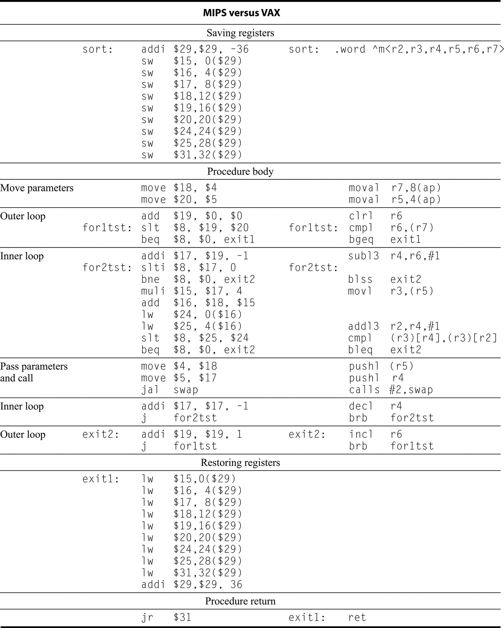
Fallacies and Pitfalls
The ability to simplify means to eliminate the unnecessary so that the necessary may speak.
Hans Hoffman
Search for the Real (1967)
- Fallacy It is possible to design a flawless architecture.
All architecture design involves trade-offs made in the context of a set of hardware and software technologies. Over time those technologies are likely to change, and decisions that may have been correct at one time later look like mistakes. For example, in 1975 the VAX designers overemphasized the importance of code size efficiency and underestimated how important ease of decoding and pipelining would be 10 years later. And, almost all architectures eventually succumb to the lack of sufficient address space. Avoiding these problems in the long run, however, would probably mean compromising the efficiency of the architecture in the short run.
- Fallacy An architecture with flaws cannot be successful.
The IBM 360 is often criticized in the literature—the branches are not PC-relative, and the address is too small in displacement addressing. Yet, the machine has been an enormous success because it correctly handled several new problems. First, the architecture has a large amount of address space. Second, it is byte addressed and handles bytes well. Third, it is a general-purpose register machine. Finally, it is simple enough to be efficiently implemented across a wide performance and cost range.
The Intel 8086 provides an even more dramatic example. The 8086 architecture is the only widespread architecture in existence today that is not truly a general-purpose register machine. Furthermore, the segmented address space of the 8086 causes major problems for both programmers and compiler writers. Nevertheless, the 8086 architecture—because of its selection as the microprocessor in the IBM PC—has been enormously successful.
- Fallacy The architecture that executes fewer instructions is faster.
Designers of VAX machines performed a quantitative comparison of VAX and MIPS for implementations with comparable organizations, the VAX 8700 and the MIPS M2000. Figure K.57 shows the ratio of the number of instructions executed and the ratio of performance measured in clock cycles. MIPS executes about twice as many instructions as the VAX while the MIPS M2000 has almost three times the performance of the VAX 8700.
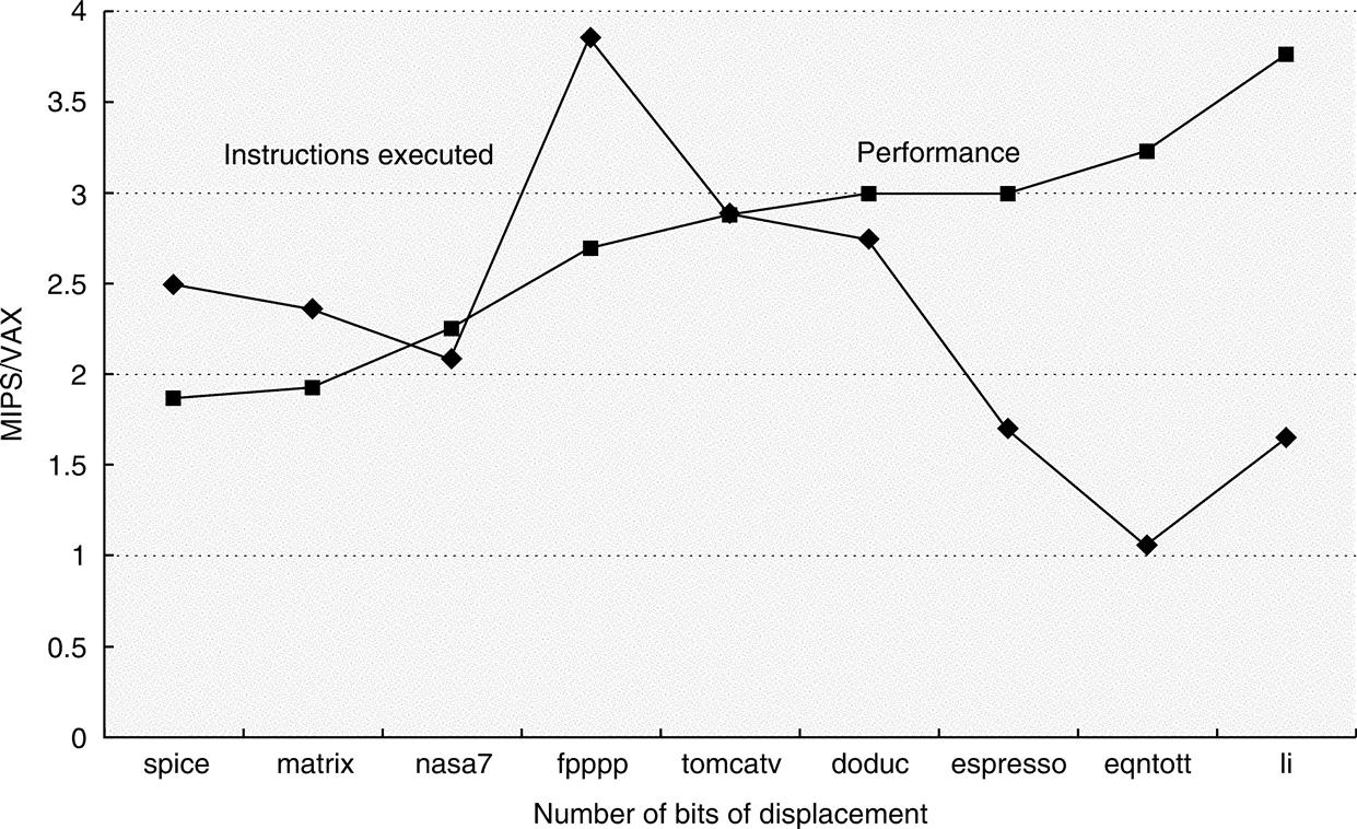
On average, MIPS executes a little over twice as many instructions as the VAX, but the CPI for the VAX is almost six times the MIPS CPI, yielding almost a threefold performance advantage. (Based on data from “Performance from Architecture: Comparing a RISC and CISC with Similar Hardware Organization,” by D. Bhandarkar and D. Clark, in Proc. Symp. Architectural Support for Programming Languages and Operating Systems IV, 1991.)
Concluding Remarks
The Virtual Address eXtension of the PDP-11 architecture … provides a virtual address of about 4.3 gigabytes which, even given the rapid improvement of memory technology, should be adequate far into the future.
William Strecker
“VAX-11/780—A Virtual Address Extension to the PDP-11 Family,” AFIPS Proc., National Computer Conference (1978)
We have seen that instruction sets can vary quite dramatically, both in how they access operands and in the operations that can be performed by a single instruction. Figure K.58 compares instruction usage for both architectures for two programs; even very different architectures behave similarly in their use of instruction classes.
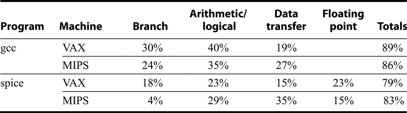
A product of its time, the VAX emphasis on code density and complex operations and addressing modes conflicts with the current emphasis on easy decoding, simple operations and addressing modes, and pipelined performance.
With more than 600,000 sold, the VAX architecture has had a very successful run. In 1991, DEC made the transition from VAX to Alpha.
Orthogonality is key to the VAX architecture; the opcode is independent of the addressing modes, which are independent of the data types and even the number of unique operands. Thus, a few hundred operations expand to hundreds of thousands of instructions when accounting for the data types, operand counts, and addressing modes.
Exercises
- K.1 [3] < K.4 > The following VAX instruction decrements the location pointed to be register r5:
decl (r5)
What is the single MIPS instruction, or if it cannot be represented in a single instruction, the shortest sequence of MIPS instructions, that performs the same operation? What are the lengths of the instructions on each machine? - K.2 [5] < K.4 > This exercise is the same as Exercise K.1, except this VAX instruction clears a location using autoincrement deferred addressing:
clrl @(r5)+ - K.3 [5] < K.4 > This exercise is the same as Exercise K.1, except this VAX instruction adds 1 to register r5, placing the sum back in register r5, compares the sum to register r6, and then branches to L1 if r5 < r6:
aoblss r6, r5, L1 # r5 = r5 + 1; if (r5 < r6) goto L1. - K.4 [5] < K.4 > Show the single VAX instruction, or minimal sequence of instructions, for this C statement:
a = b + 100;
Assume a corresponds to register r3 and b corresponds to register r4. - K.5 [10] < K.4 > Show the single VAX instruction, or minimal sequence of instructions, for this C statement:
x[i + 1] = x[i] + c;
Assume c corresponds to register r3, i to register r4, and x is an array of 32-bit words beginning at memory location 4,000,000ten.
K.5 The IBM 360/370 Architecture for Mainframe Computers
Introduction
The term “computer architecture” was coined by IBM in 1964 for use with the IBM 360. Amdahl, Blaauw, and Brooks [1964] used the term to refer to the programmer-visible portion of the instruction set. They believed that a family of machines of the same architecture should be able to run the same software. Although this idea may seem obvious to us today, it was quite novel at the time. IBM, even though it was the leading company in the industry, had five different architectures before the 360. Thus, the notion of a company standardizing on a single architecture was a radical one. The 360 designers hoped that six different divisions of IBM could be brought together by defining a common architecture. Their definition of architecture was
… the structure of a computer that a machine language programmer must understand to write a correct (timing independent) program for that machine.
The term “machine language programmer” meant that compatibility would hold, even in assembly language, while “timing independent” allowed different implementations.
The IBM 360 was introduced in 1964 with six models and a 25:1 performance ratio. Amdahl, Blaauw, and Brooks [1964] discussed the architecture of the IBM 360 and the concept of permitting multiple object-code-compatible implementations. The notion of an instruction set architecture as we understand it today was the most important aspect of the 360. The architecture also introduced several important innovations, now in wide use:
In 1971, IBM shipped the first System/370 (models 155 and 165), which included a number of significant extensions of the 360, as discussed by Case and Padegs [1978], who also discussed the early history of System/360. The most important addition was virtual memory, though virtual memory 370 s did not ship until 1972, when a virtual memory operating system was ready. By 1978, the high-end 370 was several hundred times faster than the low-end 360 s shipped 10 years earlier. In 1984, the 24-bit addressing model built into the IBM 360 needed to be abandoned, and the 370-XA (eXtended Architecture) was introduced. While old 24-bit programs could be supported without change, several instructions could not function in the same manner when extended to a 32-bit addressing model (31-bit addresses supported) because they would not produce 31-bit addresses. Converting the operating system, which was written mostly in assembly language, was no doubt the biggest task.
Several studies of the IBM 360 and instruction measurement have been made. Shustek’s thesis [1978] is the best known and most complete study of the 360/370 architecture. He made several observations about instruction set complexity that were not fully appreciated until some years later. Another important study of the 360 is the Toronto study by Alexander and Wortman [1975] done on an IBM 360 using 19 XPL programs.
System/360 Instruction Set
The 360 instruction set is shown in the following tables, organized by instruction type and format. System/370 contains 15 additional user instructions.
Integer/Logical and Floating-Point R-R Instructions
The * indicates the instruction is floating point, and may be either D (double precision) or E (single precision).
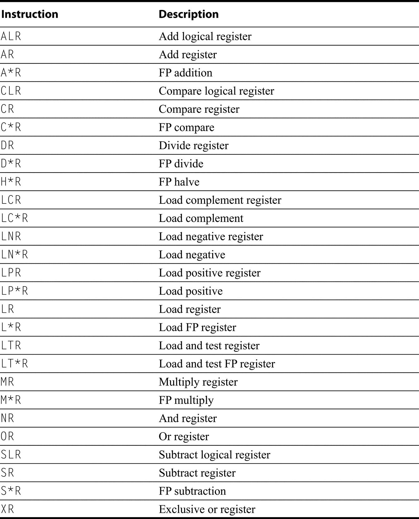
Branches and Status Setting R-R Instructions
These are R-R format instructions that either branch or set some system status; several of them are privileged and legal only in supervisor mode.
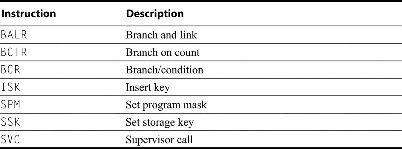
Branches/Logical and Floating-Point Instructions—RX Format
These are all RX format instructions. The symbol “+” means either a word operation (and then stands for nothing) or H (meaning half word); for example, A + stands for the two opcodes A and AH. The “*” represents D or E, standing for double- or single-precision floating point.
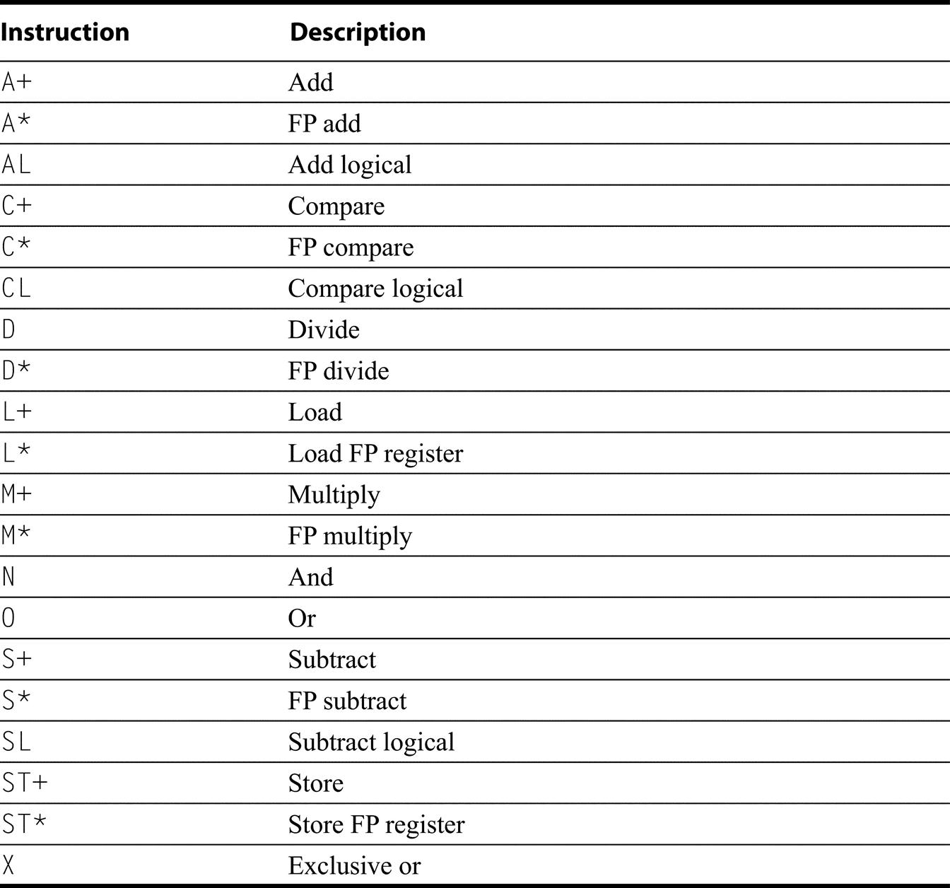
Branches and Special Loads and Stores—RX Format
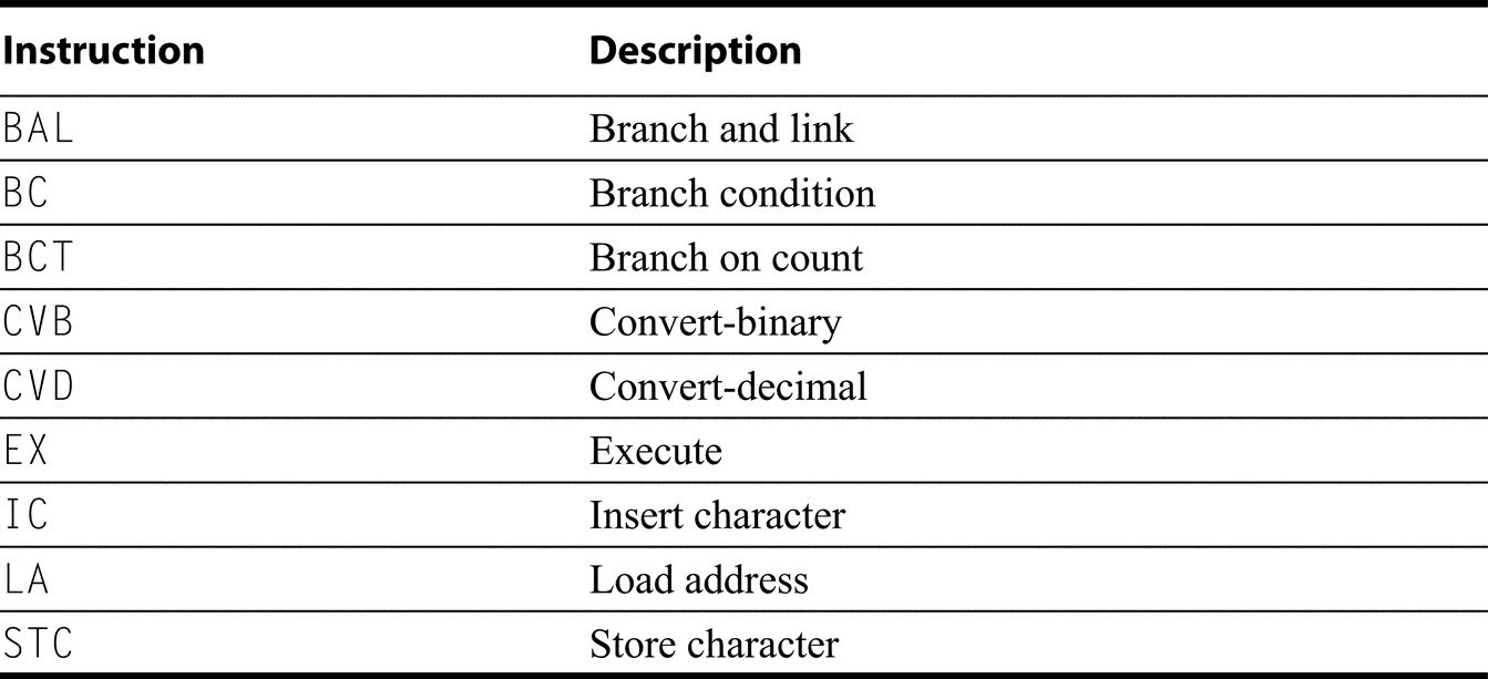
RS and SI Format Instructions
These are the RS and SI format instructions. The symbol “*” may be A (arithmetic) or L (logical).
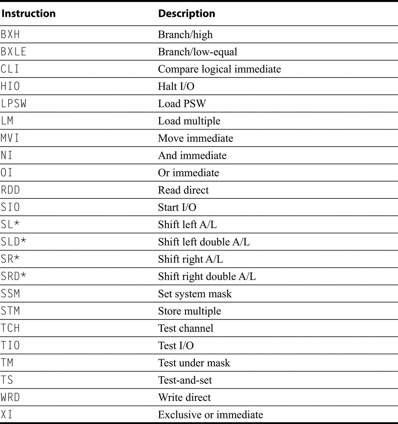
SS Format Instructions
These are add decimal or string instructions.
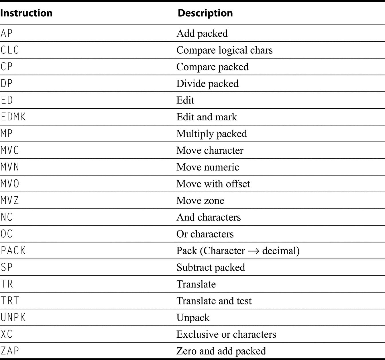
360 Detailed Measurements
Figure K.59 shows the frequency of instruction usage for four IBM 360 programs.
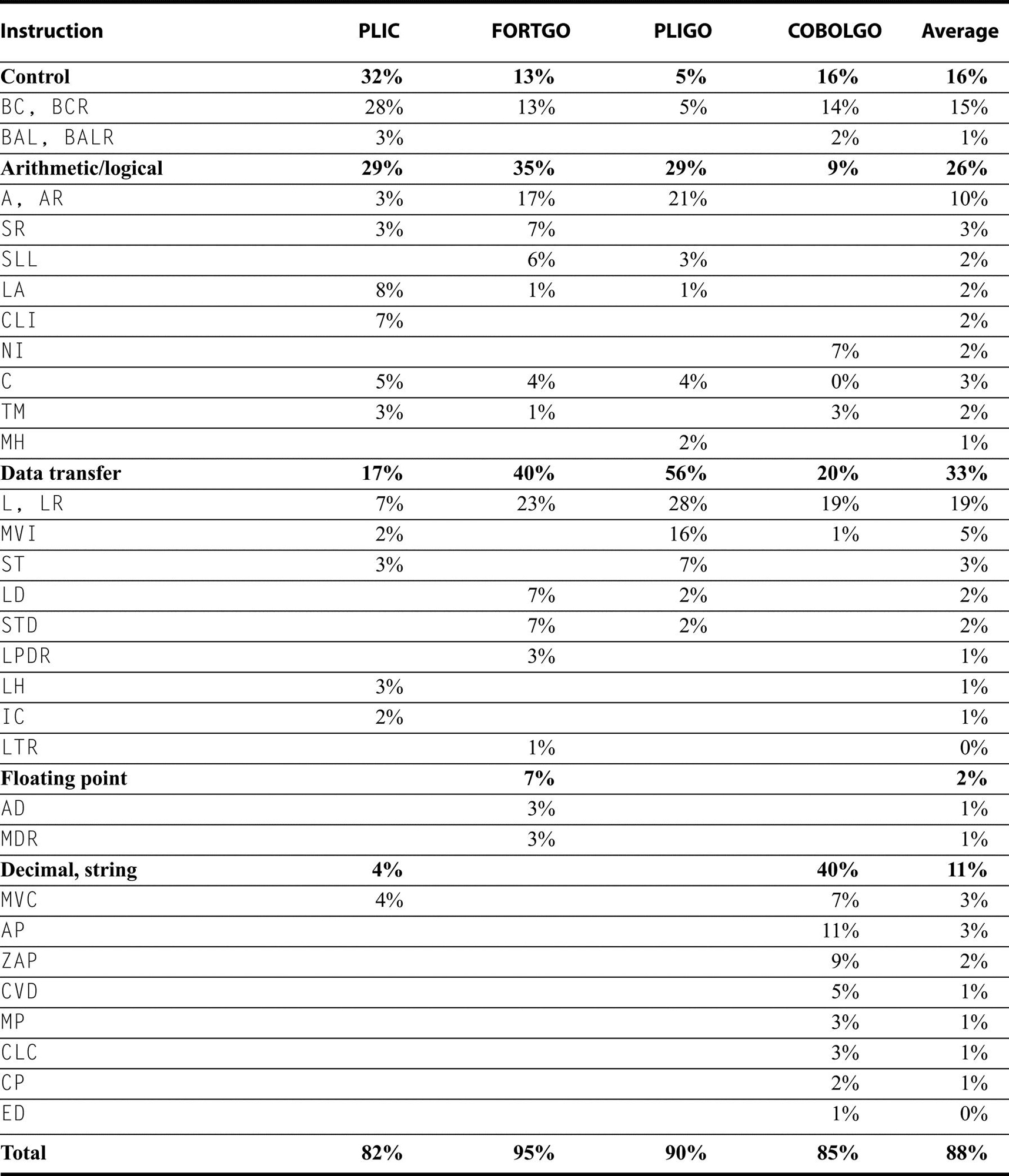
All instructions with a frequency of execution greater than 1.5% are included. Immediate instructions, which operate on only a single byte, are included in the section that characterized their operation, rather than with the long character-string versions of the same operation. By comparison, the average frequencies for the major instruction classes of the VAX are 23% (control), 28% (arithmetic), 29% (data transfer), 7% (floating point), and 9% (decimal). Once again, a 1% entry in the average column can occur because of entries in the constituent columns. These programs are a compiler for the programming language PL-I and runtime systems for the programming languages FORTRAN, PL/I, and Cobol.
K.6 Historical Perspective and References
Section L.4 (available online) features a discussion on the evolution of instruction sets and includes references for further reading and exploration of related topics.
Acknowledgments
We would like to thank the following people for comments on drafts of this survey: Professor Steven B. Furber, University of Manchester; Dr. Dileep Bhandarkar, Intel Corporation; Dr. Earl Killian, Silicon Graphics/MIPS; and Dr. Hiokazu Takata, Mitsubishi Electric Corporation.