Pipelining: Basic and Intermediate Concepts
Abstract
This appendix covers the basics of pipelining, including a discussion of the data path implications, introducing hazards, and examining the performance of pipelines.
Keywords
Data path; Hazards; Pipelining
It is quite a three-pipe problem.
Sir Arthur Conan Doyle, The Adventures of Sherlock Holmes
C.1 Introduction
Many readers of this text will have covered the basics of pipelining in another text (such as our more basic text Computer Organization and Design) or in another course. Because Chapter 3 builds heavily on this material, readers should ensure that they are familiar with the concepts discussed in this appendix before proceeding. As you read Chapter 3, you may find it helpful to turn to this material for a quick review.
We begin the appendix with the basics of pipelining, including discussing the data path implications, introducing hazards, and examining the performance of pipelines. This section describes the basic five-stage RISC pipeline that is the basis for the rest of the appendix. Section C.2 describes the issue of hazards, why they cause performance problems, and how they can be dealt with. Section C.3 discusses how the simple five-stage pipeline is actually implemented, focusing on control and how hazards are dealt with.
Section C.4 discusses the interaction between pipelining and various aspects of instruction set design, including discussing the important topic of exceptions and their interaction with pipelining. Readers unfamiliar with the concepts of precise and imprecise interrupts and resumption after exceptions will find this material useful, because they are key to understanding the more advanced approaches in Chapter 3.
Section C.5 discusses how the five-stage pipeline can be extended to handle longer-running floating-point instructions. Section C.6 puts these concepts together in a case study of a deeply pipelined processor, the MIPS R4000/4400, including both the eight-stage integer pipeline and the floating-point pipeline. The MIPS R40000 is similar to a single-issue embedded processor, such as the ARM Cortex-A5, which became available in 2010, and was used in several smart phones and tablets.
Section C.7 introduces the concept of dynamic scheduling and the use of scoreboards to implement dynamic scheduling. It is introduced as a cross-cutting issue, because it can be used to serve as an introduction to the core concepts in Chapter 3, which focused on dynamically scheduled approaches. Section C.7 is also a gentle introduction to the more complex Tomasulo’s algorithm covered in Chapter 3. Although Tomasulo’s algorithm can be covered and understood without introducing scoreboarding, the scoreboarding approach is simpler and easier to comprehend.
What Is Pipelining?
Pipelining is an implementation technique whereby multiple instructions are overlapped in execution; it takes advantage of parallelism that exists among the actions needed to execute an instruction. Today, pipelining is the key implementation technique used to make fast processors, and even processors that cost less than a dollar are pipelined.
A pipeline is like an assembly line. In an automobile assembly line, there are many steps, each contributing something to the construction of the car. Each step operates in parallel with the other steps, although on a different car. In a computer pipeline, each step in the pipeline completes a part of an instruction. Like the assembly line, different steps are completing different parts of different instructions in parallel. Each of these steps is called a pipe stage or a pipe segment. The stages are connected one to the next to form a pipe—instructions enter at one end, progress through the stages, and exit at the other end, just as cars would in an assembly line.
In an automobile assembly line, throughput is defined as the number of cars per hour and is determined by how often a completed car exits the assembly line. Likewise, the throughput of an instruction pipeline is determined by how often an instruction exits the pipeline. Because the pipe stages are hooked together, all the stages must be ready to proceed at the same time, just as we would require in an assembly line. The time required between moving an instruction one step down the pipeline is a processor cycle. Because all stages proceed at the same time, the length of a processor cycle is determined by the time required for the slowest pipe stage, just as in an auto assembly line the longest step would determine the time between advancing cars in the line. In a computer, this processor cycle is almost always 1 clock cycle.
The pipeline designer’s goal is to balance the length of each pipeline stage, just as the designer of the assembly line tries to balance the time for each step in the process. If the stages are perfectly balanced, then the time per instruction on the pipelined processor—assuming ideal conditions—is equal to

Under these conditions, the speedup from pipelining equals the number of pipe stages, just as an assembly line with n stages can ideally produce cars n times as fast. Usually, however, the stages will not be perfectly balanced; furthermore, pipelining does involve some overhead. Thus, the time per instruction on the pipelined processor will not have its minimum possible value, yet it can be close.
Pipelining yields a reduction in the average execution time per instruction. If the starting point is a processor that takes multiple clock cycles per instruction, then pipelining reduces the CPI. This is the primary view we will take.
Pipelining is an implementation technique that exploits parallelism among the instructions in a sequential instruction stream. It has the substantial advantage that, unlike some speedup techniques (see Chapter 4), it is not visible to the programmer.
The Basics of the RISC V Instruction Set
Throughout this book we use RISC V, a load-store architecture, to illustrate the basic concepts. Nearly all the ideas we introduce in this book are applicable to other processors, but the implementation may be much more complicated with complex instructions. In this section, we make use of the core of the RISC V architecture; see Chapter 1 for a full description. Although we use RISC V, the concepts are significantly similar in that they will apply to any RISC, including the core architectures of ARM and MIPS. All RISC architectures are characterized by a few key properties:
 All operations on data apply to data in registers and typically change the entire register (32 or 64 bits per register).
- The only operations that affect memory are load and store operations that move data from memory to a register or to memory from a register, respectively. Load and store operations that load or store less than a full register (e.g., a byte, 16 bits, or 32 bits) are often available.
- The instruction formats are few in number, with all instructions typically being one size. In RISC V, the register specifiers: rs1, rs2, and rd are always in the same place simplifying the control.
These simple properties lead to dramatic simplifications in the implementation of pipelining, which is why these instruction sets were designed this way. Chapter 1 contains a full description of the RISC V ISA, and we assume the reader has read Chapter 1.
A Simple Implementation of a RISC Instruction Set
To understand how a RISC instruction set can be implemented in a pipelined fashion, we need to understand how it is implemented without pipelining. This section shows a simple implementation where every instruction takes at most 5 clock cycles. We will extend this basic implementation to a pipelined version, resulting in a much lower CPI. Our unpipelined implementation is not the most economical or the highest-performance implementation without pipelining. Instead, it is designed to lead naturally to a pipelined implementation. Implementing the instruction set requires the introduction of several temporary registers that are not part of the architecture; these are introduced in this section to simplify pipelining. Our implementation will focus only on a pipeline for an integer subset of a RISC architecture that consists of load-store word, branch, and integer ALU operations.
Every instruction in this RISC subset can be implemented in, at most, 5 clock cycles. The 5 clock cycles are as follows.
- 1. Instruction fetch cycle (IF):
Send the program counter (PC) to memory and fetch the current instruction from memory. Update the PC to the next sequential instruction by adding 4 (because each instruction is 4 bytes) to the PC. - 2. Instruction decode/register fetch cycle (ID):
Decode the instruction and read the registers corresponding to register source specifiers from the register file. Do the equality test on the registers as they are read, for a possible branch. Sign-extend the offset field of the instruction in case it is needed. Compute the possible branch target address by adding the sign-extended offset to the incremented PC.
Decoding is done in parallel with reading registers, which is possible because the register specifiers are at a fixed location in a RISC architecture. This technique is known as fixed-field decoding. Note that we may read a register we don’t use, which doesn’t help but also doesn’t hurt performance. (It does waste energy to read an unneeded register, and power-sensitive designs might avoid this.) For loads and ALU immediate operations, the immediate field is always in the same place, so we can easily sign extend it. (For a more complete implementation of RISC V, we would need to compute two different sign-extended values, because the immediate field for store is in a different location.) - 3. Execution/effective address cycle (EX):
The ALU operates on the operands prepared in the prior cycle, performing one of three functions, depending on the instruction type.- Memory reference—The ALU adds the base register and the offset to form the effective address.
- Register-Register ALU instruction—The ALU performs the operation specified by the ALU opcode on the values read from the register file.
- Register-Immediate ALU instruction—The ALU performs the operation specified by the ALU opcode on the first value read from the register file and the sign-extended immediate.
- Conditional branch—Determine whether the condition is true.
In a load-store architecture the effective address and execution cycles can be combined into a single clock cycle, because no instruction needs to simultaneously calculate a data address and perform an operation on the data. - 4. Memory access (MEM):
If the instruction is a load, the memory does a read using the effective address computed in the previous cycle. If it is a store, then the memory writes the data from the second register read from the register file using the effective address. - 5. Write-back cycle (WB):
Write the result into the register file, whether it comes from the memory system (for a load) or from the ALU (for an ALU instruction).
In this implementation, branch instructions require three cycles, store instructions require four cycles, and all other instructions require five cycles. Assuming a branch frequency of 12% and a store frequency of 10%, a typical instruction distribution leads to an overall CPI of 4.66. This implementation, however, is not optimal either in achieving the best performance or in using the minimal amount of hardware given the performance level; we leave the improvement of this design as an exercise for you and instead focus on pipelining this version.
The Classic Five-Stage Pipeline for a RISC Processor
We can pipeline the execution described in the previous section with almost no changes by simply starting a new instruction on each clock cycle. (See why we chose this design?) Each of the clock cycles from the previous section becomes a pipe stage—a cycle in the pipeline. This results in the execution pattern shown in Figure C.1, which is the typical way a pipeline structure is drawn. Although each instruction takes 5 clock cycles to complete, during each clock cycle the hardware will initiate a new instruction and will be executing some part of the five different instructions.

On each clock cycle, another instruction is fetched and begins its five-cycle execution. If an instruction is started every clock cycle, the performance will be up to five times that of a processor that is not pipelined. The names for the stages in the pipeline are the same as those used for the cycles in the unpipelined implementation: IF = instruction fetch, ID = instruction decode, EX = execution, MEM = memory access, and WB = write-back.
You may find it hard to believe that pipelining is as simple as this; it’s not. In this and the following sections, we will make our RISC pipeline “real” by dealing with problems that pipelining introduces.
To start with, we have to determine what happens on every clock cycle of the processor and make sure we don’t try to perform two different operations with the same data path resource on the same clock cycle. For example, a single ALU cannot be asked to compute an effective address and perform a subtract operation at the same time. Thus, we must ensure that the overlap of instructions in the pipeline cannot cause such a conflict. Fortunately, the simplicity of a RISC instruction set makes resource evaluation relatively easy. Figure C.2 shows a simplified version of a RISC data path drawn in pipeline fashion. As you can see, the major functional units are used in different cycles, and hence overlapping the execution of multiple instructions introduces relatively few conflicts. There are three observations on which this fact rests.

This figure shows the overlap among the parts of the data path, with clock cycle 5 (CC 5) showing the steady-state situation. Because the register file is used as a source in the ID stage and as a destination in the WB stage, it appears twice. We show that it is read in one part of the stage and written in another by using a solid line, on the right or left, respectively, and a dashed line on the other side. The abbreviation IM is used for instruction memory, DM for data memory, and CC for clock cycle.
First, we use separate instruction and data memories, which we would typically implement with separate instruction and data caches (discussed in Chapter 2). The use of separate caches eliminates a conflict for a single memory that would arise between instruction fetch and data memory access. Notice that if our pipelined processor has a clock cycle that is equal to that of the unpipelined version, the memory system must deliver five times the bandwidth. This increased demand is one cost of higher performance.
Second, the register file is used in the two stages: one for reading in ID and one for writing in WB. These uses are distinct, so we simply show the register file in two places. Hence, we need to perform two reads and one write every clock cycle. To handle reads and a write to the same register (and for another reason, which will become obvious shortly), we perform the register write in the first half of the clock cycle and the read in the second half.
Third, Figure C.2 does not deal with the PC. To start a new instruction every clock, we must increment and store the PC every clock, and this must be done during the IF stage in preparation for the next instruction. Furthermore, we must also have an adder to compute the potential branch target address during ID. One further problem is that we need the ALU in the ALU stage to evaluate the branch condition. Actually, we don’t really need a full ALU to evaluate the comparison between two registers, but we need enough of the function that it has to occur in this pipestage.
Although it is critical to ensure that instructions in the pipeline do not attempt to use the hardware resources at the same time, we must also ensure that instructions in different stages of the pipeline do not interfere with one another. This separation is done by introducing pipeline registers between successive stages of the pipeline, so that at the end of a clock cycle all the results from a given stage are stored into a register that is used as the input to the next stage on the next clock cycle. Figure C.3 shows the pipeline drawn with these pipeline registers.

Notice that the registers prevent interference between two different instructions in adjacent stages in the pipeline. The registers also play the critical role of carrying data for a given instruction from one stage to the other. The edge-triggered property of registers—that is, that the values change instantaneously on a clock edge—is critical. Otherwise, the data from one instruction could interfere with the execution of another!
Although many figures will omit such registers for simplicity, they are required to make the pipeline operate properly and must be present. Of course, similar registers would be needed even in a multicycle data path that had no pipelining (because only values in registers are preserved across clock boundaries). In the case of a pipelined processor, the pipeline registers also play the key role of carrying intermediate results from one stage to another where the source and destination may not be directly adjacent. For example, the register value to be stored during a store instruction is read during ID, but not actually used until MEM; it is passed through two pipeline registers to reach the data memory during the MEM stage. Likewise, the result of an ALU instruction is computed during EX, but not actually stored until WB; it arrives there by passing through two pipeline registers. It is sometimes useful to name the pipeline registers, and we follow the convention of naming them by the pipeline stages they connect, so the registers are called IF/ID, ID/EX, EX/MEM, and MEM/WB.
Basic Performance Issues in Pipelining
Pipelining increases the processor instruction throughput—the number of instructions completed per unit of time—but it does not reduce the execution time of an individual instruction. In fact, it usually slightly increases the execution time of each instruction due to overhead in the control of the pipeline. The increase in instruction throughput means that a program runs faster and has lower total execution time, even though no single instruction runs faster!
The fact that the execution time of each instruction does not decrease puts limits on the practical depth of a pipeline, as we will see in the next section. In addition to limitations arising from pipeline latency, limits arise from imbalance among the pipe stages and from pipelining overhead. Imbalance among the pipe stages reduces performance because the clock can run no faster than the time needed for the slowest pipeline stage. Pipeline overhead arises from the combination of pipeline register delay and clock skew. The pipeline registers add setup time, which is the time that a register input must be stable before the clock signal that triggers a write occurs, plus propagation delay to the clock cycle. Clock skew, which is the maximum delay between when the clock arrives at any two registers, also contributes to the lower limit on the clock cycle. Once the clock cycle is as small as the sum of the clock skew and latch overhead, no further pipelining is useful, because there is no time left in the cycle for useful work. The interested reader should see Kunkel and Smith (1986).
Example
Consider the unpipelined processor in the previous section. Assume that it has a 4 GHz clock (or a 0.5 ns clock cycle) and that it uses four cycles for ALU operations and branches and five cycles for memory operations. Assume that the relative frequencies of these operations are 40%, 20%, and 40%, respectively. Suppose that due to clock skew and setup, pipelining the processor adds 0.1 ns of overhead to the clock. Ignoring any latency impact, how much speedup in the instruction execution rate will we gain from a pipeline?
Answer
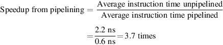
The average instruction execution time on the unpipelined processor is

In the pipelined implementation, the clock must run at the speed of the slowest stage plus overhead, which will be 0.5 + 0.1 or 0.6 ns; this is the average instruction execution time. Thus, the speedup from pipelining is
The 0.1 ns overhead essentially establishes a limit on the effectiveness of pipelining. If the overhead is not affected by changes in the clock cycle, Amdahl’s Law tells us that the overhead limits the speedup.
This simple RISC pipeline would function just fine for integer instructions if every instruction were independent of every other instruction in the pipeline. In reality, instructions in the pipeline can depend on one another; this is the topic of the next section.
C.2 The Major Hurdle of Pipelining—Pipeline Hazards
There are situations, called hazards, that prevent the next instruction in the instruction stream from executing during its designated clock cycle. Hazards reduce the performance from the ideal speedup gained by pipelining. There are three classes of hazards:
- 1. Structural hazards arise from resource conflicts when the hardware cannot support all possible combinations of instructions simultaneously in overlapped execution. In modern processors, structural hazards occur primarily in special purpose functional units that are less frequently used (such as floating point divide or other complex long running instructions). They are not a major performance factor, assuming programmers and compiler writers are aware of the lower throughput of these instructions. Instead of spending more time on this infrequent case, we focus on the two other hazards that are much more frequent.
- 2. Data hazards arise when an instruction depends on the results of a previous instruction in a way that is exposed by the overlapping of instructions in the pipeline.
- 3. Control hazards arise from the pipelining of branches and other instructions that change the PC.
Hazards in pipelines can make it necessary to stall the pipeline. Avoiding a hazard often requires that some instructions in the pipeline be allowed to proceed while others are delayed. For the pipelines we discuss in this appendix, when an instruction is stalled, all instructions issued later than the stalled instruction—and hence not as far along in the pipeline—are also stalled. Instructions issued earlier than the stalled instruction—and hence farther along in the pipeline—must continue, because otherwise the hazard will never clear. As a result, no new instructions are fetched during the stall. We will see several examples of how pipeline stalls operate in this section—don’t worry, they aren’t as complex as they might sound!
Performance of Pipelines With Stalls
A stall causes the pipeline performance to degrade from the ideal performance. Let’s look at a simple equation for finding the actual speedup from pipelining, starting with the formula from the previous section:

Pipelining can be thought of as decreasing the CPI or the clock cycle time. Because it is traditional to use the CPI to compare pipelines, let’s start with that assumption. The ideal CPI on a pipelined processor is almost always 1. Hence, we can compute the pipelined CPI:

If we ignore the cycle time overhead of pipelining and assume that the stages are perfectly balanced, then the cycle time of the two processors can be equal, leading to

One important simple case is where all instructions take the same number of cycles, which must also equal the number of pipeline stages (also called the depth of the pipeline). In this case, the unpipelined CPI is equal to the depth of the pipeline, leading to

If there are no pipeline stalls, this leads to the intuitive result that pipelining can improve performance by the depth of the pipeline.
Data Hazards
A major effect of pipelining is to change the relative timing of instructions by overlapping their execution. This overlap introduces data and control hazards. Data hazards occur when the pipeline changes the order of read/write accesses to operands so that the order differs from the order seen by sequentially executing instructions on an unpipelined processor. Assume instruction i occurs in program order before instruction j and both instructions use register x, then there are three different types of hazards that can occur between i and j:
- 1. Read After Write (RAW) hazard: the most common, these occur when a read of register x by instruction j occurs before the write of register x by instruction i. If this hazard were not prevented instruction j would use the wrong value of x.
- 2. Write After Read (WAR) hazard: this hazard occurs when read of register x by instruction i occurs after a write of register x by instruction j. In this case, instruction i would use the wrong value of x. WAR hazards are impossible in the simple five stage, integrer pipeline, but they occur when instructions are reordered, as we will see when we discuss dynamically scheduled pipelines beginning on page C.65.
- 3. Write After Write (WAW) hazard: this hazard occurs when write of register x by instruction i occurs after a write of register x by instruction j. When this occurs, register x will have the wrong value going forward. WAR hazards are also impossible in the simple five stage, integrer pipeline, but they occur when instructions are reordered or when running times vary, as we will see later.
Chapter 3 explores the issues of data dependence and hazards in much more detail. For now, we focus only on RAW hazards.
Consider the pipelined execution of these instructions:
add      x1,x2,x3
sub      x4,x1,x5
and      x6,x1,x7
or       x8,x1,x9
xor      x10,x1,x11
All the instructions after the add use the result of the add instruction. As shown in Figure C.4, the add instruction writes the value of x1 in the WB pipe stage, but the sub instruction reads the value during its ID stage, which results in a RAW hazard. Unless precautions are taken to prevent it, the sub instruction will read the wrong value and try to use it. In fact, the value used by the sub instruction is not even deterministic: though we might think it logical to assume that sub would always use the value of x1 that was assigned by an instruction prior to add, this is not always the case. If an interrupt should occur between the add and sub instructions, the WB stage of the add will complete, and the value of x1 at that point will be the result of the add. This unpredictable behavior is obviously unacceptable.

The and instruction also creates a possible RAW hazard. As we can see from Figure C.4, the write of x1 does not complete until the end of clock cycle 5. Thus, the and instruction that reads the registers during clock cycle 4 will receive the wrong results.
The xor instruction operates properly because its register read occurs in clock cycle 6, after the register write. The or instruction also operates without incurring a hazard because we perform the register file reads in the second half of the cycle and the writes in the first half. Note that the xor instruction still depends on the add, but it no longer creates a hazard; a topic we explore in more detail in Chapter 3.
The next subsection discusses a technique to eliminate the stalls for the hazard involving the sub and and instructions.
Minimizing Data Hazard Stalls by Forwarding
The problem posed in Figure C.4 can be solved with a simple hardware technique called forwarding (also called bypassing and sometimes short-circuiting). The key insight in forwarding is that the result is not really needed by the sub until after the add actually produces it. If the result can be moved from the pipeline register where the add stores it to where the sub needs it, then the need for a stall can be avoided. Using this observation, forwarding works as follows:
- 1. The ALU result from both the EX/MEM and MEM/WB pipeline registers is always fed back to the ALU inputs.
- 2. If the forwarding hardware detects that the previous ALU operation has written the register corresponding to a source for the current ALU operation, control logic selects the forwarded result as the ALU input rather than the value read from the register file.
Notice that with forwarding, if the sub is stalled, the add will be completed and the bypass will not be activated. This relationship is also true for the case of an interrupt between the two instructions.
As the example in Figure C.4 shows, we need to forward results not only from the immediately previous instruction but also possibly from an instruction that started two cycles earlier. Figure C.5 shows our example with the bypass paths in place and highlighting the timing of the register read and writes. This code sequence can be executed without stalls.

The inputs for the sub and and instructions forward from the pipeline registers to the first ALU input. The or receives its result by forwarding through the register file, which is easily accomplished by reading the registers in the second half of the cycle and writing in the first half, as the dashed lines on the registers indicate. Notice that the forwarded result can go to either ALU input; in fact, both ALU inputs could use forwarded inputs from either the same pipeline register or from different pipeline registers. This would occur, for example, if the and instruction was and x6,x1,x4.
Forwarding can be generalized to include passing a result directly to the functional unit that requires it: a result is forwarded from the pipeline register corresponding to the output of one unit to the input of another, rather than just from the result of a unit to the input of the same unit. Take, for example, the following sequence:
add      x1,x2,x3
ld       x4,0(x1)
sd       x4,12(x1)
To prevent a stall in this sequence, we would need to forward the values of the ALU output and memory unit output from the pipeline registers to the ALU and data memory inputs. Figure C.6 shows all the forwarding paths for this example.

The result of the load is forwarded from the memory output to the memory input to be stored. In addition, the ALU output is forwarded to the ALU input for the address calculation of both the load and the store (this is no different than forwarding to another ALU operation). If the store depended on an immediately preceding ALU operation (not shown herein), the result would need to be forwarded to prevent a stall.
Data Hazards Requiring Stalls
Unfortunately, not all potential data hazards can be handled by bypassing. Consider the following sequence of instructions:
ld       x1,0(x2)
sub      x4,x1,x5
and      x6,x1,x7
or       x8,x1,x9
The pipelined data path with the bypass paths for this example is shown in Figure C.7. This case is different from the situation with back-to-back ALU operations. The ld instruction does not have the data until the end of clock cycle 4 (its MEM cycle), while the sub instruction needs to have the data by the beginning of that clock cycle. Thus, the data hazard from using the result of a load instruction cannot be completely eliminated with simple hardware. As Figure C.7 shows, such a forwarding path would have to operate backward in time—a capability not yet available to computer designers! We can forward the result immediately to the ALU from the pipeline registers for use in the and operation, which begins 2 clock cycles after the load. Likewise, the or instruction has no problem, because it receives the value through the register file. For the sub instruction, the forwarded result arrives too late—at the end of a clock cycle, when it is needed at the beginning.

The load instruction has a delay or latency that cannot be eliminated by forwarding alone. Instead, we need to add hardware, called a pipeline interlock, to preserve the correct execution pattern. In general, a pipeline interlock detects a hazard and stalls the pipeline until the hazard is cleared. In this case, the interlock stalls the pipeline, beginning with the instruction that wants to use the data until the source instruction produces it. This pipeline interlock introduces a stall or bubble, just as it did for the structural hazard. The CPI for the stalled instruction increases by the length of the stall (1 clock cycle in this case).
Figure C.8 shows the pipeline before and after the stall using the names of the pipeline stages. Because the stall causes the instructions starting with the sub to move one cycle later in time, the forwarding to the and instruction now goes through the register file, and no forwarding at all is needed for the or instruction. The insertion of the bubble causes the number of cycles to complete this sequence to grow by one. No instruction is started during clock cycle 4 (and none finishes during cycle 6).

Branch Hazards
Control hazards can cause a greater performance loss for our RISC V pipeline than do data hazards. When a branch is executed, it may or may not change the PC to something other than its current value plus 4. Recall that if a branch changes the PC to its target address, it is a taken branch; if it falls through, it is not taken, or untaken. If instruction i is a taken branch, then the PC is usually not changed until the end of ID, after the completion of the address calculation and comparison.
Figure C.9 shows that the simplest method of dealing with branches is to redo the fetch of the instruction following a branch, once we detect the branch during ID (when instructions are decoded). The first IF cycle is essentially a stall, because it never performs useful work. You may have noticed that if the branch is untaken, then the repetition of the IF stage is unnecessary because the correct instruction was indeed fetched. We will develop several schemes to take advantage of this fact shortly.

The instruction after the branch is fetched, but the instruction is ignored, and the fetch is restarted once the branch target is known. It is probably obvious that if the branch is not taken, the second IF for branch successor is redundant. This will be addressed shortly.
One stall cycle for every branch will yield a performance loss of 10% to 30% depending on the branch frequency, so we will examine some techniques to deal with this loss.
Reducing Pipeline Branch Penalties
There are many methods for dealing with the pipeline stalls caused by branch delay; we discuss four simple compile time schemes in this subsection. In these four schemes the actions for a branch are static—they are fixed for each branch during the entire execution. The software can try to minimize the branch penalty using knowledge of the hardware scheme and of branch behavior. We will then look at hardware-based schemes that dynamically predict branch behavior, and Chapter 3 looks at more powerful hardware techniques for dynamic branch prediction.
The simplest scheme to handle branches is to freeze or flush the pipeline, holding or deleting any instructions after the branch until the branch destination is known. The attractiveness of this solution lies primarily in its simplicity both for hardware and software. It is the solution used earlier in the pipeline shown in Figure C.9. In this case, the branch penalty is fixed and cannot be reduced by software.
A higher-performance, and only slightly more complex, scheme is to treat every branch as not taken, simply allowing the hardware to continue as if the branch were not executed. Here, care must be taken not to change the processor state until the branch outcome is definitely known. The complexity of this scheme arises from having to know when the state might be changed by an instruction and how to “back out” such a change.
In the simple five-stage pipeline, this predicted-not-taken or predicted-untaken scheme is implemented by continuing to fetch instructions as if the branch were a normal instruction. The pipeline looks as if nothing out of the ordinary is happening. If the branch is taken, however, we need to turn the fetched instruction into a no-op and restart the fetch at the target address. Figure C.10 shows both situations.

When the branch is untaken, determined during ID, we fetch the fall-through and just continue. If the branch is taken during ID, we restart the fetch at the branch target. This causes all instructions following the branch to stall 1 clock cycle.
An alternative scheme is to treat every branch as taken. As soon as the branch is decoded and the target address is computed, we assume the branch to be taken and begin fetching and executing at the target. This buys us a one-cycle improvement when the branch is actually taken, because we know the target address at the end of ID, one cycle before we know whether the branch condition is satisfied in the ALU stage. In either a predicted-taken or predicted-not-taken scheme, the compiler can improve performance by organizing the code so that the most frequent path matches the hardware’s choice.
A fourth scheme, which was heavily used in early RISC processors is called delayed branch. In a delayed branch, the execution cycle with a branch delay of one is
branch instruction
sequential successor1
branch target if taken
The sequential successor is in the branch delay slot. This instruction is executed whether or not the branch is taken. The pipeline behavior of the five-stage pipeline with a branch delay is shown in Figure C.11. Although it is possible to have a branch delay longer than one, in practice almost all processors with delayed branch have a single instruction delay; other techniques are used if the pipeline has a longer potential branch penalty. The job of the compiler is to make the successor instructions valid and useful.

The instructions in the delay slot (there was only one delay slot for most RISC architectures that incorporated them) are executed. If the branch is untaken, execution continues with the instruction after the branch delay instruction; if the branch is taken, execution continues at the branch target. When the instruction in the branch delay slot is also a branch, the meaning is unclear: if the branch is not taken, what should happen to the branch in the branch delay slot? Because of this confusion, architectures with delay branches often disallow putting a branch in the delay slot.
Although the delayed branch was useful for short simple pipelines at a time when hardware prediction was too expensive, the technique complicates implementation when there is dynamic branch prediction. For this reason, RISC V appropriately omitted delayed branches.
Performance of Branch Schemes
What is the effective performance of each of these schemes? The effective pipeline speedup with branch penalties, assuming an ideal CPI of 1, is

Because of the following:

we obtain:

The branch frequency and branch penalty can have a component from both unconditional and conditional branches. However, the latter dominate because they are more frequent.
Example
For a deeper pipeline, such as that in a MIPS R4000 and later RISC processors, it takes at least three pipeline stages before the branch-target address is known and an additional cycle before the branch condition is evaluated, assuming no stalls on the registers in the conditional comparison. A three-stage delay leads to the branch penalties for the three simplest prediction schemes listed in Figure C.12.

Find the effective addition to the CPI arising from branches for this pipeline, assuming the following frequencies:
| Unconditional branch | 4% |
| Conditional branch, untaken | 6% |
| Conditional branch, taken | 10% |
Answer
We find the CPIs by multiplying the relative frequency of unconditional, conditional untaken, and conditional taken branches by the respective penalties. The results are shown in Figure C.13.

The differences among the schemes are substantially increased with this longer delay. If the base CPI were 1 and branches were the only source of stalls, the ideal pipeline would be 1.56 times faster than a pipeline that used the stall-pipeline scheme. The predicted-untaken scheme would be 1.13 times better than the stall-pipeline scheme under the same assumptions.
Reducing the Cost of Branches Through Prediction
As pipelines get deeper and the potential penalty of branches increases, using delayed branches and similar schemes becomes insufficient. Instead, we need to turn to more aggressive means for predicting branches. Such schemes fall into two classes: low-cost static schemes that rely on information available at compile time and strategies that predict branches dynamically based on program behavior. We discuss both approaches here.
Static Branch Prediction
A key way to improve compile-time branch prediction is to use profile information collected from earlier runs. The key observation that makes this worthwhile is that the behavior of branches is often bimodally distributed; that is, an individual branch is often highly biased toward taken or untaken. Figure C.14 shows the success of branch prediction using this strategy. The same input data were used for runs and for collecting the profile; other studies have shown that changing the input so that the profile is for a different run leads to only a small change in the accuracy of profile-based prediction.

The actual performance depends on both the prediction accuracy and the branch frequency, which vary from 3% to 24%.
The effectiveness of any branch prediction scheme depends both on the accuracy of the scheme and the frequency of conditional branches, which vary in SPEC from 3% to 24%. The fact that the misprediction rate for the integer programs is higher and such programs typically have a higher branch frequency is a major limitation for static branch prediction. In the next section, we consider dynamic branch predictors, which most recent processors have employed.
Dynamic Branch Prediction and Branch-Prediction Buffers
The simplest dynamic branch-prediction scheme is a branch-prediction buffer or branch history table. A branch-prediction buffer is a small memory indexed by the lower portion of the address of the branch instruction. The memory contains a bit that says whether the branch was recently taken or not. This scheme is the simplest sort of buffer; it has no tags and is useful only to reduce the branch delay when it is longer than the time to compute the possible target PCs.
With such a buffer, we don’t know, in fact, if the prediction is correct—it may have been put there by another branch that has the same low-order address bits. But this doesn’t matter. The prediction is a hint that is assumed to be correct, and fetching begins in the predicted direction. If the hint turns out to be wrong, the prediction bit is inverted and stored back.
This buffer is effectively a cache where every access is a hit, and, as we will see, the performance of the buffer depends on both how often the prediction is for the branch of interest and how accurate the prediction is when it matches. Before we analyze the performance, it is useful to make a small, but important, improvement in the accuracy of the branch-prediction scheme.
This simple 1-bit prediction scheme has a performance shortcoming: even if a branch is almost always taken, we will likely predict incorrectly twice, rather than once, when it is not taken, because the misprediction causes the prediction bit to be flipped.
To remedy this weakness, 2-bit prediction schemes are often used. In a 2-bit scheme, a prediction must miss twice before it is changed. Figure C.15 shows the finite-state processor for a 2-bit prediction scheme.

By using 2 bits rather than 1, a branch that strongly favors taken or not taken—as many branches do—will be mispredicted less often than with a 1-bit predictor. The 2 bits are used to encode the four states in the system. The 2-bit scheme is actually a specialization of a more general scheme that has an n-bit saturating counter for each entry in the prediction buffer. With an n-bit counter, the counter can take on values between 0 and 2n − 1: when the counter is greater than or equal to one-half of its maximum value (2n − 1), the branch is predicted as taken; otherwise, it is predicted as untaken. Studies of n-bit predictors have shown that the 2-bit predictors do almost as well, thus most systems rely on 2-bit branch predictors rather than the more general n-bit predictors.
A branch-prediction buffer can be implemented as a small, special “cache” accessed with the instruction address during the IF pipe stage, or as a pair of bits attached to each block in the instruction cache and fetched with the instruction. If the instruction is decoded as a branch and if the branch is predicted as taken, fetching begins from the target as soon as the PC is known. Otherwise, sequential fetching and executing continue. As Figure C.15 shows, if the prediction turns out to be wrong, the prediction bits are changed.
What kind of accuracy can be expected from a branch-prediction buffer using 2 bits per entry on real applications? Figure C.16 shows that for the SPEC89 benchmarks a branch-prediction buffer with 4096 entries results in a prediction accuracy ranging from over 99% to 82%, or a misprediction rate of 1%–18%. A 4K entry buffer, like that used for these results, is considered small in 2017, and a larger buffer could produce somewhat better results.

The misprediction rate for the integer benchmarks (gcc, espresso, eqntott, and li) is substantially higher (average of 11%) than that for the floating-point programs (average of 4%). Omitting the floating-point kernels (nasa7, matrix300, and tomcatv) still yields a higher accuracy for the FP benchmarks than for the integer benchmarks. These data, as well as the rest of the data in this section, are taken from a branch-prediction study done using the IBM Power architecture and optimized code for that system. See Pan et al. (1992). Although these data are for an older version of a subset of the SPEC benchmarks, the newer benchmarks are larger and would show slightly worse behavior, especially for the integer benchmarks.
As we try to exploit more ILP, the accuracy of our branch prediction becomes critical. As we can see in Figure C.16, the accuracy of the predictors for integer programs, which typically also have higher branch frequencies, is lower than for the loop-intensive scientific programs. We can attack this problem in two ways: by increasing the size of the buffer and by increasing the accuracy of the scheme we use for each prediction. A buffer with 4K entries, however, as Figure C.17 shows, performs quite comparably to an infinite buffer, at least for benchmarks like those in SPEC. The data in Figure C.17 make it clear that the hit rate of the buffer is not the major limiting factor. As we mentioned, simply increasing the number of bits per predictor without changing the predictor structure also has little impact. Instead, we need to look at how we might increase the accuracy of each predictor, as we will in Chapter 3.

Although these data are for an older version of a subset of the SPEC benchmarks, the results would be comparable for newer versions with perhaps as many as 8K entries needed to match an infinite 2-bit predictor.
C.3 How Is Pipelining Implemented?
Before we proceed to basic pipelining, we need to review a simple implementation of an unpipelined version of RISC V.
A Simple Implementation of RISC V
In this section we follow the style of Section C.1, showing first a simple unpipelined implementation and then the pipelined implementation. This time, however, our example is specific to the RISC V architecture.
In this subsection, we focus on a pipeline for an integer subset of RISC V that consists of load-store word, branch equal, and integer ALU operations. Later in this appendix we will incorporate the basic floating-point operations. Although we discuss only a subset of RISC V, the basic principles can be extended to handle all the instructions; for example, adding store involves some additional computing of the immediate field. We initially used a less aggressive implementation of a branch instruction. We show how to implement the more aggressive version at the end of this section.
Every RISC V instruction can be implemented in, at most, 5 clock cycles. The 5 clock cycles are as follows:
Operation—Send out the PC and fetch the instruction from memory into the instruction register (IR); increment the PC by 4 to address the next sequential instruction. The IR is used to hold the instruction that will be needed on subsequent clock cycles; likewise, the register NPC is used to hold the next sequential PC.
Operation—Decode the instruction and access the register file to read the registers (rs1 and rs2 are the register specifiers). The outputs of the general-purpose registers are read into two temporary registers (A and B) for use in later clock cycles. The lower 16 bits of the IR are also sign extended and stored into the temporary register Imm, for use in the next cycle.
Decoding is done in parallel with reading registers, which is possible because these fields are at a fixed location in the RISC V instruction format. Because the immediate portion of a load and an ALU immediate is located in an identical place in every RISC V instruction, the sign-extended immediate is also calculated during this cycle in case it is needed in the next cycle. For stores, a separate sign-extension is needed, because the immediate field is split in two pieces.
The ALU operates on the operands prepared in the prior cycle, performing one of four functions depending on the RISC V instruction type:
Operation—The ALU adds the operands to form the effective address and places the result into the register ALUOutput.
Operation—The ALU performs the operation specified by the function code (a combination of the func3 and func7 fields) on the value in register A and on the value in register B. The result is placed in the temporary register ALUOutput.
Operation—The ALU performs the operation specified by the opcode on the value in register A and on the value in register Imm. The result is placed in the temporary register ALUOutput.
Operation—The ALU adds the NPC to the sign-extended immediate value in Imm, which is shifted left by 2 bits to create a word offset, to compute the address of the branch target. Register A, which has been read in the prior cycle, is checked to determine whether the branch is taken, by comparison with Register B, because we consider only branch equal.
The load-store architecture of RISC V means that effective address and execution cycles can be combined into a single clock cycle, because no instruction needs to simultaneously calculate a data address, calculate an instruction target address, and perform an operation on the data. The other integer instructions not included herein are jumps of various forms, which are similar to branches.
The PC is updated for all instructions: PC ← NPC;
Operation—Access memory if needed. If the instruction is a load, data return from memory and are placed in the LMD (load memory data) register; if it is a store, then the data from the B register are written into memory. In either case, the address used is the one computed during the prior cycle and stored in the register ALUOutput.
Operation—If the instruction branches, the PC is replaced with the branch destination address in the register ALUOutput.
Operation—Write the result into the register file, whether it comes from the memory system (which is in LMD) or from the ALU (which is in ALUOutput) with rd designating the register.
Figure C.18 shows how an instruction flows through the data path. At the end of each clock cycle, every value computed during that clock cycle and required on a later clock cycle (whether for this instruction or the next) is written into a storage device, which may be memory, a general-purpose register, the PC, or a temporary register (i.e., LMD, Imm, A, B, IR, NPC, ALUOutput, or Cond). The temporary registers hold values between clock cycles for one instruction, while the other storage elements are visible parts of the state and hold values between successive instructions.

Although the PC is shown in the portion of the data path that is used in instruction fetch and the registers are shown in the portion of the data path that is used in instruction decode/register fetch, both of these functional units are read as well as written by an instruction. Although we show these functional units in the cycle corresponding to where they are read, the PC is written during the memory access clock cycle and the registers are written during the write-back clock cycle. In both cases, the writes in later pipe stages are indicated by the multiplexer output (in memory access or write-back), which carries a value back to the PC or registers. These backward-flowing signals introduce much of the complexity of pipelining, because they indicate the possibility of hazards.
Although all processors today are pipelined, this multicycle implementation is a reasonable approximation of how most processors would have been implemented in earlier times. A simple finite-state machine could be used to implement the control following the five-cycle structure shown herein. For a much more complex processor, microcode control could be used. In either event, an instruction sequence like the one described in this section would determine the structure of the control.
There are some hardware redundancies that could be eliminated in this multicycle implementation. For example, there are two ALUs: one to increment the PC and one used for effective address and ALU computation. Because they are not needed on the same clock cycle, we could merge them by adding additional multiplexers and sharing the same ALU. Likewise, instructions and data could be stored in the same memory, because the data and instruction accesses happen on different clock cycles.
Rather than optimize this simple implementation, we will leave the design as it is in Figure C.18, because this provides us with a better base for the pipelined implementation.
A Basic Pipeline for RISC V
As before, we can pipeline the data path of Figure C.18 with almost no changes by starting a new instruction on each clock cycle. Because every pipe stage is active on every clock cycle, all operations in a pipe stage must complete in 1 clock cycle and any combination of operations must be able to occur at once. Furthermore, pipelining the data path requires that values passed from one pipe stage to the next must be placed in registers. Figure C.19 shows the RISC V pipeline with the appropriate registers, called pipeline registers or pipeline latches, between each pipeline stage. The registers are labeled with the names of the stages they connect. Figure C.19 is drawn so that connections through the pipeline registers from one stage to another are clear.

The registers serve to convey values and control information from one stage to the next. We can also think of the PC as a pipeline register, which sits before the IF stage of the pipeline, leading to one pipeline register for each pipe stage. Recall that the PC is an edge-triggered register written at the end of the clock cycle; hence, there is no race condition in writing the PC. The selection multiplexer for the PC has been moved so that the PC is written in exactly one stage (IF). If we didn’t move it, there would be a conflict when a branch occurred, because two instructions would try to write different values into the PC. Most of the data paths flow from left to right, which is from earlier in time to later. The paths flowing from right to left (which carry the register write-back information and PC information on a branch) introduce complications into our pipeline.
All of the registers needed to hold values temporarily between clock cycles within one instruction are subsumed into these pipeline registers. The fields of the instruction register (IR), which is part of the IF/ID register, are labeled when they are used to supply register names. The pipeline registers carry both data and control from one pipeline stage to the next. Any value needed on a later pipeline stage must be placed in such a register and copied from one pipeline register to the next, until it is no longer needed. If we tried to just use the temporary registers we had in our earlier unpipelined data path, values could be overwritten before all uses were completed. For example, the field of a register operand used for a write on a load or ALU operation is supplied from the MEM/WB pipeline register rather than from the IF/ID register. This is because we want a load or ALU operation to write the register designated by that operation, not the register field of the instruction currently transitioning from IF to ID! This destination register field is simply copied from one pipeline register to the next, until it is needed during the WB stage.
Any instruction is active in exactly one stage of the pipeline at a time; therefore, any actions taken on behalf of an instruction occur between a pair of pipeline registers. Thus, we can also look at the activities of the pipeline by examining what has to happen on any pipeline stage depending on the instruction type. Figure C.20 shows this view. Fields of the pipeline registers are named so as to show the flow of data from one stage to the next. Notice that the actions in the first two stages are independent of the current instruction type; they must be independent because the instruction is not decoded until the end of the ID stage. The IF activity depends on whether the instruction in EX/MEM is a taken branch. If so, then the branch-target address of the branch instruction in EX/MEM is written into the PC at the end of IF; otherwise, the incremented PC will be written back. (As we said earlier, this effect of branches leads to complications in the pipeline that we deal with in the next few sections.) The fixed-position encoding of the register source operands is critical to allowing the registers to be fetched during ID.

Let’s review the actions in the stages that are specific to the pipeline organization. In IF, in addition to fetching the instruction and computing the new PC, we store the incremented PC both into the PC and into a pipeline register (NPC) for later use in computing the branch-target address. This structure is the same as the organization in Figure C.19, where the PC is updated in IF from one of two sources. In ID, we fetch the registers, extend the sign of the 12 bits of the IR (the immediate field), and pass along the IR and NPC. During EX, we perform an ALU operation or an address calculation; we pass along the IR and the B register (if the instruction is a store). We also set the value of cond to 1 if the instruction is a taken branch. During the MEM phase, we cycle the memory, write the PC if needed, and pass along values needed in the final pipe stage. Finally, during WB, we update the register field from either the ALU output or the loaded value. For simplicity we always pass the entire IR from one stage to the next, although as an instruction proceeds down the pipeline, less and less of the IR is needed.
To control this simple pipeline we need only determine how to set the control for the four multiplexers in the data path of Figure C.19. The two multiplexers in the ALU stage are set depending on the instruction type, which is dictated by the IR field of the ID/EX register. The top ALU input multiplexer is set by whether the instruction is a branch or not, and the bottom multiplexer is set by whether the instruction is a register-register ALU operation or any other type of operation. The multiplexer in the IF stage chooses whether to use the value of the incremented PC or the value of the EX/MEM.ALUOutput (the branch target) to write into the PC. This multiplexer is controlled by the field EX/MEM.cond. The fourth multiplexer is controlled by whether the instruction in the WB stage is a load or an ALU operation. In addition to these four multiplexers, there is one additional multiplexer needed that is not drawn in Figure C.19, but whose existence is clear from looking at the WB stage of an ALU operation. The destination register field is in one of two different places depending on the instruction type (register-register ALU versus either ALU immediate or load). Thus, we will need a multiplexer to choose the correct portion of the IR in the MEM/WB register to specify the register destination field, assuming the instruction writes a register.
Implementing the Control for the RISC V Pipeline
The process of letting an instruction move from the instruction decode stage (ID) into the execution stage (EX) of this pipeline is usually called instruction issue; an instruction that has made this step is said to have issued. For the RISC V integer pipeline, all the data hazards can be checked during the ID phase of the pipeline. If a data hazard exists, the instruction is stalled before it is issued. Likewise, we can determine what forwarding will be needed during ID and set the appropriate controls then. Detecting interlocks early in the pipeline reduces the hardware complexity because the hardware never has to suspend an instruction that has updated the state of the processor, unless the entire processor is stalled. Alternatively, we can detect the hazard or forwarding at the beginning of a clock cycle that uses an operand (EX and MEM for this pipeline). To show the differences in these two approaches, we will show how the interlock for a read after write (RAW) hazard with the source coming from a load instruction (called a load interlock) can be implemented by a check in ID, while the implementation of forwarding paths to the ALU inputs can be done during EX. Figure C.21 lists the variety of circumstances that we must handle.

This table indicates that the only comparison needed is between the destination and the sources on the two instructions following the instruction that wrote the destination. In the case of a stall, the pipeline dependences will look like the third case once execution continues (dependence overcome by forwarding). Of course, hazards that involve x0 can be ignored because the register always contains 0, and the preceding test could be extended to do this.
Let’s start with implementing the load interlock. If there is a RAW hazard with the source instruction being a load, the load instruction will be in the EX stage when an instruction that needs the load data will be in the ID stage. Thus, we can describe all the possible hazard situations with a small table, which can be directly translated to an implementation. Figure C.22 shows a table that detects all load interlocks when the instruction using the load result is in the ID stage.

Remember that the IF/ID register holds the state of the instruction in ID, which potentially uses the load result, while ID/EX holds the state of the instruction in EX, which is the load instruction.
Once a hazard has been detected, the control unit must insert the pipeline stall and prevent the instructions in the IF and ID stages from advancing. As we said earlier, all the control information is carried in the pipeline registers. (Carrying the instruction along is enough, because all control is derived from it.) Thus, when we detect a hazard we need only change the control portion of the ID/EX pipeline register to all 0s, which happens to be a no-op (an instruction that does nothing, such as add x0,x0,x0). In addition, we simply recirculate the contents of the IF/ID registers to hold the stalled instruction. In a pipeline with more complex hazards, the same ideas would apply: we can detect the hazard by comparing some set of pipeline registers and shift in no-ops to prevent erroneous execution.
Implementing the forwarding logic is similar, although there are more cases to consider. The key observation needed to implement the forwarding logic is that the pipeline registers contain both the data to be forwarded as well as the source and destination register fields. All forwarding logically happens from the ALU or data memory output to the ALU input, the data memory input, or the zero detection unit. Thus, we can implement the forwarding by a comparison of the destination registers of the IR contained in the EX/MEM and MEM/WB stages against the source registers of the IR contained in the ID/EX and EX/MEM registers. Figure C.23 shows the comparisons and possible forwarding operations where the destination of the forwarded result is an ALU input for the instruction currently in EX.

There are 10 separate comparisons needed to tell whether a forwarding operation should occur. The top and bottom ALU inputs refer to the inputs corresponding to the first and second ALU source operands, respectively, and are shown explicitly in Figure C.18 on page C.30 and in Figure C.24 on page C.36. Remember that the pipeline latch for destination instruction in EX is ID/EX, while the source values come from the ALUOutput portion of EX/MEM or MEM/WB or the LMD portion of MEM/WB. There is one complication not addressed by this logic: dealing with multiple instructions that write the same register. For example, during the code sequence add x1, x2, x3; addi x1, x1, 2; sub x4, x3, x1, the logic must ensure that the sub instruction uses the result of the addi instruction rather than the result of the add instruction. The logic shown here can be extended to handle this case by simply testing that forwarding from MEM/WB is enabled only when forwarding from EX/MEM is not enabled for the same input. Because the addi result will be in EX/MEM, it will be forwarded, rather than the add result in MEM/WB.
In addition to the comparators and combinational logic that we must determine when a forwarding path needs to be enabled, we also must enlarge the multiplexers at the ALU inputs and add the connections from the pipeline registers that are used to forward the results. Figure C.24 shows the relevant segments of the pipelined data path with the additional multiplexers and connections in place.

The paths correspond to a bypass of: (1) the ALU output at the end of the EX, (2) the ALU output at the end of the MEM stage, and (3) the memory output at the end of the MEM stage.
For RISC V, the hazard detection and forwarding hardware is reasonably simple; we will see that things become somewhat more complicated when we extend this pipeline to deal with floating point. Before we do that, we need to handle branches.
Dealing With Branches in the Pipeline
In RISC V, conditional branches depend on comparing two register values, which we assume occurs during the EX cycle, and uses the ALU for this function. We will need to also compute the branch target address. Because testing the branch condition and determining the next PC will determine what the branch penalty is, we would like to compute both the possible PCs and choose the correct PC before the end of the EX cycle. We can do this by adding a separate adder that computes the branch target address during ID. Because the instruction is not yet decoded, we will be computing a possible target as if every instruction were a branch. This is likely faster than computing the target and evaluating the condition both in EX, but does use slightly more energy.
Figure C.25 shows a pipelined data path assuming the adder in ID and the evaluation of the branch condition in EX, a minor change of the pipeline structure. This pipeline will incur a two-cycle penalty on branches. In some early RISC processors, such as MIPS, the condition test on branches was restricted to allow the test to occur in ID, reducing the branch delay to one cycle. Of course, that meant that an ALU operation to a register followed by a conditional branch based on that register incurred a data hazard, which does not occur if the branch condition is evaluated in EX.

As mentioned in Figure C.19, the PC can be thought of as a pipeline register (e.g., as part of ID/IF), which is written with the address of the next instruction at the end of each IF cycle.
As pipeline depths increased, the branch delay increased, which made dynamic branch prediction necessary. For example, a processor with separate decode and register fetch stages will probably have a branch delay that is at least 1 clock cycle longer. The branch delay, unless it is dealt with, turns into a branch penalty. Many older processors that implement more complex instruction sets have branch delays of 4 clock cycles or more, and large, deeply pipelined processors often have branch penalties of 6 or 7. Aggressive high-end superscalars, such as the Intel i7 discussed in Chapter 3, may have branch penalties of 10–15 cycles! In general, the deeper the pipeline, the worse the branch penalty in clock cycles, and the more critical that branches be accurately predicted.
C.4 What Makes Pipelining Hard to Implement?
Now that we understand how to detect and resolve hazards, we can deal with some complications that we have avoided so far. The first part of this section considers the challenges of exceptional situations where the instruction execution order is changed in unexpected ways. In the second part of this section, we discuss some of the challenges raised by different instruction sets.
Dealing With Exceptions
Exceptional situations are harder to handle in a pipelined processor because the overlapping of instructions makes it more difficult to know whether an instruction can safely change the state of the processor. In a pipelined processor, an instruction is executed piece by piece and is not completed for several clock cycles. Unfortunately, other instructions in the pipeline can raise exceptions that may force the processor to abort the instructions in the pipeline before they complete. Before we discuss these problems and their solutions in detail, we need to understand what types of situations can arise and what architectural requirements exist for supporting them.
Types of Exceptions and Requirements
The terminology used to describe exceptional situations where the normal execution order of instruction is changed varies among processors. The terms interrupt, fault, and exception are used, although not in a consistent fashion. We use the term exception to cover all these mechanisms, including the following:
- I/O device request
- Invoking an operating system service from a user program
- Tracing instruction execution
- Breakpoint (programmer-requested interrupt)
- Integer arithmetic overflow
- FP arithmetic anomaly
- Page fault (not in main memory)
- Misaligned memory accesses (if alignment is required)
- Memory protection violation
- Using an undefined or unimplemented instruction
- Hardware malfunctions
- Power failure
When we wish to refer to some particular class of such exceptions, we will use a longer name, such as I/O interrupt, floating-point exception, or page fault.
Although we use the term exception to cover all of these events, individual events have important characteristics that determine what action is needed in the hardware. The requirements on exceptions can be characterized on five semi-independent axes:
- 1. Synchronous versus asynchronous—If the event occurs at the same place every time the program is executed with the same data and memory allocation, the event is synchronous. With the exception of hardware malfunctions, asynchronous events are caused by devices external to the processor and memory. Asynchronous events usually can be handled after the completion of the current instruction, which makes them easier to handle.
- 2. User requested versus coerced—If the user task directly asks for it, it is a user-requested event. In some sense, user-requested exceptions are not really exceptions, because they are predictable. They are treated as exceptions, however, because the same mechanisms that are used to save and restore the state are used for these user-requested events. Because the only function of an instruction that triggers this exception is to cause the exception, user-requested exceptions can always be handled after the instruction has completed. Coerced exceptions are caused by some hardware event that is not under the control of the user program. Coerced exceptions are harder to implement because they are not predictable.
- 3. User maskable versus user nonmaskable—If an event can be masked or disabled by a user task, it is user maskable. This mask simply controls whether the hardware responds to the exception or not.
- 4. Within versus between instructions—This classification depends on whether the event prevents instruction completion by occurring in the middle of execution—no matter how short—or whether it is recognized between instructions. Exceptions that occur within instructions are usually synchronous, because the instruction triggers the exception. It’s harder to implement exceptions that occur within instructions than those between instructions, because the instruction must be stopped and restarted. Asynchronous exceptions that occur within instructions arise from catastrophic situations (e.g., hardware malfunction) and always cause program termination.
- 5. Resume versus terminate—If the program’s execution always stops after the interrupt, it is a terminating event. If the program’s execution continues after the interrupt, it is a resuming event. It is easier to implement exceptions that terminate execution, because the processor need not be able to restart execution of the same program after handling the exception.
Figure C.26 classifies the preceding examples according to these five categories. The difficult task is implementing interrupts occurring within instructions where the instruction must be resumed. Implementing such exceptions requires that another program must be invoked to save the state of the executing program, correct the cause of the exception, and then restore the state of the program before the instruction that caused the exception can be tried again. This process must be effectively invisible to the executing program. If a pipeline provides the ability for the processor to handle the exception, save the state, and restart without affecting the execution of the program, the pipeline or processor is said to be restartable. While early supercomputers and microprocessors often lacked this property, almost all processors today support it, at least for the integer pipeline, because it is needed to implement virtual memory (see Chapter 2).

Exceptions that must allow resumption are marked as resume, although the software may often choose to terminate the program. Synchronous, coerced exceptions occurring within instructions that can be resumed are the most difficult to implement. We might expect that memory protection access violations would always result in termination; however, modern operating systems use memory protection to detect events such as the first attempt to use a page or the first write to a page. Thus, processors should be able to resume after such exceptions.
Stopping and Restarting Execution
As in unpipelined implementations, the most difficult exceptions have two properties: (1) they occur within instructions (that is, in the middle of the instruction execution corresponding to EX or MEM pipe stages), and (2) they must be restartable. In our RISC V pipeline, for example, a virtual memory page fault resulting from a data fetch cannot occur until sometime in the MEM stage of the instruction. By the time that fault is seen, several other instructions will be in execution. A page fault must be restartable and requires the intervention of another process, such as the operating system. Thus, the pipeline must be safely shut down and the state saved so that the instruction can be restarted in the correct state. Restarting is usually implemented by saving the PC of the instruction at which to restart. If the restarted instruction is not a branch, then we will continue to fetch the sequential successors and begin their execution in the normal fashion. If the restarted instruction is a branch, then we will reevaluate the branch condition and begin fetching from either the target or the fall-through. When an exception occurs, the pipeline control can take the following steps to save the pipeline state safely:
- 1. Force a trap instruction into the pipeline on the next IF.
- 2. Until the trap is taken, turn off all writes for the faulting instruction and for all instructions that follow in the pipeline; this can be done by placing zeros into the pipeline latches of all instructions in the pipeline, starting with the instruction that generates the exception, but not those that precede that instruction. This prevents any state changes for instructions that will not be completed before the exception is handled.
- 3. After the exception-handling routine in the operating system receives control, it immediately saves the PC of the faulting instruction. This value will be used to return from the exception later.
After the exception has been handled, special instructions return the processor from the exception by reloading the PCs and restarting the instruction stream (using the exception return in RISC V). If the pipeline can be stopped so that the instructions just before the faulting instruction are completed and those after it can be restarted from scratch, the pipeline is said to have precise exceptions. Ideally, the faulting instruction would not have changed the state, and correctly handling some exceptions requires that the faulting instruction have no effects. For other exceptions, such as floating-point exceptions, the faulting instruction on some processors writes its result before the exception can be handled. In such cases, the hardware must be prepared to retrieve the source operands, even if the destination is identical to one of the source operands. Because floating-point operations may run for many cycles, it is highly likely that some other instruction may have written the source operands (as we will see in the next section, floating-point operations often complete out of order). To overcome this, many recent high-performance processors have introduced two modes of operation. One mode has precise exceptions and the other (fast or performance mode) does not. Of course, the precise exception mode is slower, since it allows less overlap among floating-point instructions.
Supporting precise exceptions is a requirement in many systems, while in others it is “just” valuable because it simplifies the operating system interface. At a minimum, any processor with demand paging or IEEE arithmetic trap handlers must make its exceptions precise, either in the hardware or with some software support. For integer pipelines, the task of creating precise exceptions is easier, and accommodating virtual memory strongly motivates the support of precise exceptions for memory references. In practice, these reasons have led designers and architects to always provide precise exceptions for the integer pipeline. In this section we describe how to implement precise exceptions for the RISC V integer pipeline. We will describe techniques for handling the more complex challenges arising in the floating-point pipeline in Section C.5.
Exceptions in RISC V
Figure C.27 shows the RISC V pipeline stages and which problem exceptions might occur in each stage. With pipelining, multiple exceptions may occur in the same clock cycle because there are multiple instructions in execution. For example, consider this instruction sequence:

Exceptions raised from instruction or data memory access account for six out of eight cases.
This pair of instructions can cause a data page fault and an arithmetic exception at the same time, because the ld is in the MEM stage while the add is in the EX stage. This case can be handled by dealing with only the data page fault and then restarting the execution. The second exception will reoccur (but not the first, if the software is correct), and when the second exception occurs it can be handled independently.
In reality, the situation is not as straightforward as this simple example. Exceptions may occur out of order; that is, an instruction may cause an exception before an earlier instruction causes one. Consider again the preceding sequence of instructions, ld followed by add. The ld can get a data page fault, seen when the instruction is in MEM, and the add can get an instruction page fault, seen when the add instruction is in IF. The instruction page fault will actually occur first, even though it is caused by a later instruction!
Because we are implementing precise exceptions, the pipeline is required to handle the exception caused by the ld instruction first. To explain how this works, let’s call the instruction in the position of the ld instruction i, and the instruction in the position of the add instruction i + 1. The pipeline cannot simply handle an exception when it occurs in time, because that will lead to exceptions occurring out of the unpipelined order. Instead, the hardware posts all exceptions caused by a given instruction in a status vector associated with that instruction. The exception status vector is carried along as the instruction goes down the pipeline. Once an exception indication is set in the exception status vector, any control signal that may cause a data value to be written is turned off (this includes both register writes and memory writes). Because a store can cause an exception during MEM, the hardware must be prepared to prevent the store from completing if it raises an exception.
When an instruction enters WB (or is about to leave MEM), the exception status vector is checked. If any exceptions are posted, they are handled in the order in which they would occur in time on an unpipelined processor—the exception corresponding to the earliest instruction (and usually the earliest pipe stage for that instruction) is handled first. This guarantees that all exceptions will be seen on instruction i before any are seen on i + 1. Of course, any action taken in earlier pipe stages on behalf of instruction i may be invalid, but because writes to the register file and memory were disabled, no state could have been changed. As we will see in Section C.5, maintaining this precise model for FP operations is much harder.
In the next subsection we describe problems that arise in implementing exceptions in the pipelines of processors with more powerful, longer-running instructions.
Instruction Set Complications
No RISC V instruction has more than one result, and our RISC V pipeline writes that result only at the end of an instruction’s execution. When an instruction is guaranteed to complete, it is called committed. In the RISC V integer pipeline, all instructions are committed when they reach the end of the MEM stage (or beginning of WB) and no instruction updates the state before that stage. Thus, precise exceptions are straightforward. Some processors have instructions that change the state in the middle of the instruction execution, before the instruction and its predecessors are guaranteed to complete. For example, autoincrement addressing modes in the IA-32 architecture cause the update of registers in the middle of an instruction execution. In such a case, if the instruction is aborted because of an exception, it will leave the processor state altered. Although we know which instruction caused the exception, without additional hardware support the exception will be imprecise because the instruction will be half finished. Restarting the instruction stream after such an imprecise exception is difficult. Alternatively, we could avoid updating the state before the instruction commits, but this may be difficult or costly, because there may be dependences on the updated state: consider a VAX instruction that autoincrements the same register multiple times. Thus, to maintain a precise exception model, most processors with such instructions have the ability to back out any state changes made before the instruction is committed. If an exception occurs, the processor uses this ability to reset the state of the processor to its value before the interrupted instruction started. In the next section, we will see that a more powerful RISC V floating-point pipeline can introduce similar problems, and Section C.7 introduces techniques that substantially complicate exception handling.
A related source of difficulties arises from instructions that update memory state during execution, such as the string copy operations on the Intel architecture or IBM 360 (see Appendix K). To make it possible to interrupt and restart these instructions, the instructions are defined to use the general-purpose registers as working registers. Thus, the state of the partially completed instruction is always in the registers, which are saved on an exception and restored after the exception, allowing the instruction to continue.
A different set of difficulties arises from odd bits of state that may create additional pipeline hazards or may require extra hardware to save and restore. Condition codes are a good example of this. Many processors set the condition codes implicitly as part of the instruction. This approach has advantages, because condition codes decouple the evaluation of the condition from the actual branch. However, implicitly set condition codes can cause difficulties in scheduling any pipeline delays between setting the condition code and the branch, because most instructions set the condition code and cannot be used in the delay slots between the condition evaluation and the branch.
Additionally, in processors with condition codes, the processor must decide when the branch condition is fixed. This involves finding out when the condition code has been set for the last time before the branch. In most processors with implicitly set condition codes, this is done by delaying the branch condition evaluation until all previous instructions have had a chance to set the condition code.
Of course, architectures with explicitly set condition codes allow the delay between condition test and the branch to be scheduled; however, pipeline control must still track the last instruction that sets the condition code to know when the branch condition is decided. In effect, the condition code must be treated as an operand that requires hazard detection for RAW hazards with branches, just as RISC V must do on the registers.
A final thorny area in pipelining is multicycle operations. Imagine trying to pipeline a sequence of x86 instructions such as this:
mov       BX, AX       ; moves between registers
add       42(BX+SI),BX ;adds memory contents and register
                       ; to same memory location
sub       BX,AX        ;subtracts registers
rep movsb              ;moves a character string of
                       ; length given by register CX
Although none of these instructions is particularly long (an x86 instruction can be up to 15 bytes), they do differ radically in the number of clock cycles they will require, from as low as one up to hundreds of clock cycles. These instructions also require different numbers of data memory accesses, from zero to possibly hundreds. The data hazards are very complex and occur both between and within instructions (nothing prevents the movsb from having an overlapping source and destination!). The simple solution of making all instructions execute for the same number of clock cycles is unacceptable because it introduces an enormous number of hazards and bypass conditions and makes an immensely long pipeline. Pipelining the x86 at the instruction level is difficult, but a clever solution was found, similar to one used for the VAX. They pipeline the microinstruction execution; a microinstruction is a simple instruction used in sequences to implement a more complex instruction set. Because the microinstructions are simple (they look a lot like RISC V), the pipeline control is much easier. Since 1995, all Intel IA-32 microprocessors have used this strategy of converting the IA-32 instructions into microoperations, and then pipelining the microoperations. In fact, this approach is even used for some of the more complex instructions in the ARM architecture.
In comparison, load-store processors have simple operations with similar amounts of work and pipeline more easily. If architects realize the relationship between instruction set design and pipelining, they can design architectures for more efficient pipelining. In the next section, we will see how the RISC V pipeline deals with long-running instructions, specifically floating-point operations.
For many years, the interaction between instruction sets and implementations was believed to be small, and implementation issues were not a major focus in designing instruction sets. In the 1980s, it became clear that the difficulty and inefficiency of pipelining could both be increased by instruction set complications. In the 1990s, all companies moved to simpler instructions sets with the goal of reducing the complexity of aggressive implementations.
C.5 Extending the RISC V Integer Pipeline to Handle Multicycle Operations
We now want to explore how our RISC V pipeline can be extended to handle floating-point operations. This section concentrates on the basic approach and the design alternatives, closing with some performance measurements of a RISC V floating-point pipeline.
It is impractical to require that all RISC V FP operations complete in 1 clock cycle, or even in 2. Doing so would mean accepting a slow clock or using enormous amounts of logic in the FP units, or both. Instead, the FP pipeline will allow for a longer latency for operations. This is easier to grasp if we imagine the FP instructions as having the same pipeline as the integer instructions, with two important changes. First, the EX cycle may be repeated as many times as needed to complete the operation—the number of repetitions can vary for different operations. Second, there may be multiple FP functional units. A stall will occur if the instruction to be issued will cause either a structural hazard for the functional unit it uses or a data hazard.
For this section, let’s assume that there are four separate functional units in our RISC V implementation:
If we also assume that the execution stages of these functional units are not pipelined, then Figure C.28 shows the resulting pipeline structure. Because EX is not pipelined, no other instruction using that functional unit may issue until the previous instruction leaves EX. Moreover, if an instruction cannot proceed to the EX stage, the entire pipeline behind that instruction will be stalled.

Because only one instruction issues on every clock cycle, all instructions go through the standard pipeline for integer operations. The FP operations simply loop when they reach the EX stage. After they have finished the EX stage, they proceed to MEM and WB to complete execution.
In reality, the intermediate results are probably not cycled around the EX unit as Figure C.28 suggests; instead, the EX pipeline stage has some number of clock delays larger than 1. We can generalize the structure of the FP pipeline shown in Figure C.28 to allow pipelining of some stages and multiple ongoing operations. To describe such a pipeline, we must define both the latency of the functional units and also the initiation interval or repeat interval. We define latency the same way we defined it earlier: the number of intervening cycles between an instruction that produces a result and an instruction that uses the result. The initiation or repeat interval is the number of cycles that must elapse between issuing two operations of a given type. For example, we will use the latencies and initiation intervals shown in Figure C.29.

With this definition of latency, integer ALU operations have a latency of 0, because the results can be used on the next clock cycle, and loads have a latency of 1, because their results can be used after one intervening cycle. Because most operations consume their operands at the beginning of EX, the latency is usually the number of stages after EX that an instruction produces a result—for example, zero stages for ALU operations and one stage for loads. The primary exception is stores, which consume the value being stored one cycle later. Hence, the latency to a store for the value being stored, but not for the base address register, will be one cycle less. Pipeline latency is essentially equal to one cycle less than the depth of the execution pipeline, which is the number of stages from the EX stage to the stage that produces the result. Thus, for the preceding example pipeline, the number of stages in an FP add is four, while the number of stages in an FP multiply is seven. To achieve a higher clock rate, designers need to put fewer logic levels in each pipe stage, which makes the number of pipe stages required for more complex operations larger. The penalty for the faster clock rate is thus longer latency for operations.
The example pipeline structure in Figure C.29 allows up to four outstanding FP adds, seven outstanding FP/integer multiplies, and one FP divide. Figure C.30 shows how this pipeline can be drawn by extending Figure C.28. The repeat interval is implemented in Figure C.30 by adding additional pipeline stages, which will be separated by additional pipeline registers. Because the units are independent, we name the stages differently. The pipeline stages that take multiple clock cycles, such as the divide unit, are further subdivided to show the latency of those stages. Because they are not complete stages, only one operation may be active. The pipeline structure can also be shown using the familiar diagrams from earlier in the appendix, as Figure C.31 shows for a set of independent FP operations and FP loads and stores. Naturally, the longer latency of the FP operations increases the frequency of RAW hazards and resultant stalls, as we will see later in this section.

The FP multiplier and adder are fully pipelined and have a depth of seven and four stages, respectively. The FP divider is not pipelined, but requires 24 clock cycles to complete. The latency in instructions between the issue of an FP operation and the use of the result of that operation without incurring a RAW stall is determined by the number of cycles spent in the execution stages. For example, the fourth instruction after an FP add can use the result of the FP add. For integer ALU operations, the depth of the execution pipeline is always one and the next instruction can use the results.

The stages in italics show where data are needed, while the stages in bold show where a result is available. FP loads and stores use a 64-bit path to memory so that the pipelining timing is just like an integer load or store.
The structure of the pipeline in Figure C.30 requires the introduction of the additional pipeline registers (e.g.,A1/A2, A2/A3, A3/A4) and the modification of the connections to those registers. The ID/EX register must be expanded to connect ID to EX, DIV, M1, and A1; we can refer to the portion of the register associated with one of the next stages with the notation ID/EX, ID/DIV, ID/M1, or ID/A1. The pipeline register between ID and all the other stages may be thought of as logically separate registers and may, in fact, be implemented as separate registers. Because only one operation can be in a pipe stage at a time, the control information can be associated with the register at the head of the stage.
Hazards and Forwarding in Longer Latency Pipelines
There are a number of different aspects to the hazard detection and forwarding for a pipeline like that shown in Figure C.30.
- 1. Because the divide unit is not fully pipelined, structural hazards can occur. These will need to be detected and issuing instructions will need to be stalled.
- 2. Because the instructions have varying running times, the number of register writes required in a cycle can be larger than 1.
- 3. Write after write (WAW) hazards are possible, because instructions no longer reach WB in order. Note that write after read (WAR) hazards are not possible, because the register reads always occur in ID.
- 4. Instructions can complete in a different order than they were issued, causing problems with exceptions; we deal with this in the next subsection.
- 5. Because of longer latency of operations, stalls for RAW hazards will be more frequent.
The increase in stalls arising from longer operation latencies is fundamentally the same as that for the integer pipeline. Before describing the new problems that arise in this FP pipeline and looking at solutions, let’s examine the potential impact of RAW hazards. Figure C.32 shows a typical FP code sequence and the resultant stalls. At the end of this section, we’ll examine the performance of this FP pipeline for our SPEC subset.

The longer pipeline substantially raises the frequency of stalls versus the shallower integer pipeline. Each instruction in this sequence is dependent on the previous and proceeds as soon as data are available, which assumes the pipeline has full bypassing and forwarding. The fsd must be stalled an extra cycle so that its MEM does not conflict with the fadd.d. Extra hardware could easily handle this case.
Now look at the problems arising from writes, described as (2) and (3) in the earlier list. If we assume that the FP register file has one write port, sequences of FP operations, as well as an FP load together with FP operations, can cause conflicts for the register write port. Consider the pipeline sequence shown in Figure C.33. In clock cycle 11, all three instructions will reach WB and want to write the register file. With only a single register file write port, the processor must serialize the instruction completion. This single register port represents a structural hazard. We could increase the number of write ports to solve this, but that solution may be unattractive because the additional write ports would be used only rarely. This is because the maximum steady-state number of write ports needed is 1. Instead, we choose to detect and enforce access to the write port as a structural hazard.

This is not the worst case, because an earlier divide in the FP unit could also finish on the same clock. Note that although the fmul.d, fadd.d, and fld are in the MEM stage in clock cycle 10, only the fld actually uses the memory, so no structural hazard exists for MEM.
There are two different ways to implement this interlock. The first is to track the use of the write port in the ID stage and to stall an instruction before it issues, just as we would for any other structural hazard. Tracking the use of the write port can be done with a shift register that indicates when already-issued instructions will use the register file. If the instruction in ID needs to use the register file at the same time as an instruction already issued, the instruction in ID is stalled for a cycle. On each clock the reservation register is shifted 1 bit. This implementation has an advantage: It maintains the property that all interlock detection and stall insertion occurs in the ID stage. The cost is the addition of the shift register and write conflict logic. We will assume this scheme throughout this section.
An alternative scheme is to stall a conflicting instruction when it tries to enter either the MEM or WB stage. If we wait to stall the conflicting instructions until they want to enter the MEM or WB stage, we can choose to stall either instruction. A simple, though sometimes suboptimal, heuristic is to give priority to the unit with the longest latency, because that is the one most likely to have caused another instruction to be stalled for a RAW hazard. The advantage of this scheme is that it does not require us to detect the conflict until the entrance of the MEM or WB stage, where it is easy to see. The disadvantage is that it complicates pipeline control, as stalls can now arise from two places. Notice that stalling before entering MEM will cause the EX, A4, or M7 stage to be occupied, possibly forcing the stall to trickle back in the pipeline. Likewise, stalling before WB would cause MEM to back up.
Our other problem is the possibility of WAW hazards. To see that these exist, consider the example in Figure C.33. If the fadd.d instruction were issued one cycle earlier and had a destination of f2, then it would create a WAW hazard, because it would write f2 one cycle earlier than the fadd.d. Note that this hazard only occurs when the result of the fadd.d is overwritten without any instruction ever using it! If there were a use of f2 between the fadd.d and the fadd.d, the pipeline would need to be stalled for a RAW hazard, and the fadd.d would not issue until the fadd.d was completed. We could argue that, for our pipeline, WAW hazards only occur when a useless instruction is executed, but we must still detect them and make sure that the result of the fadd.d appears in f2 when we are done. (As we will see in Section C.8, such sequences sometimes do occur in reasonable code.)
There are two possible ways to handle this WAW hazard. The first approach is to delay the issue of the load instruction until the fadd.d enters MEM. The second approach is to stamp out the result of the fadd.d by detecting the hazard and changing the control so that the fadd.d does not write its result. Then the fadd.d can issue right away. Because this hazard is rare, either scheme will work fine—you can pick whatever is simpler to implement. In either case, the hazard can be detected during ID when the fadd.d is issuing, and stalling the fadd.d or making the fadd.d a no-op is easy. The difficult situation is to detect that the fadd.d might finish before the fadd.d, because that requires knowing the length of the pipeline and the current position of the fadd.d. Luckily, this code sequence (two writes with no intervening read) will be very rare, so we can use a simple solution: if an instruction in ID wants to write the same register as an instruction already issued, do not issue the instruction to EX. In Section C.7, we will see how additional hardware can eliminate stalls for such hazards. First, let’s put together the pieces for implementing the hazard and issue logic in our FP pipeline.
In detecting the possible hazards, we must consider hazards among FP instructions, as well as hazards between an FP instruction and an integer instruction. Except for FP loads-stores and FP-integer register moves, the FP and integer registers are distinct. All integer instructions operate on the integer registers, while the FP operations operate only on their own registers. Thus, we need only consider FP loads-stores and FP register moves in detecting hazards between FP and integer instructions. This simplification of pipeline control is an additional advantage of having separate register files for integer and floating-point data. (The main advantages are a doubling of the number of registers, without making either set larger, and an increase in bandwidth without adding more ports to either set. The main disadvantage, beyond the need for an extra register file, is the small cost of occasional moves needed between the two register sets.) Assuming that the pipeline does all hazard detection in ID, there are three checks that must be performed before an instruction can issue:
- 1. Check for structural hazards—Wait until the required functional unit is not busy (this is only needed for divides in this pipeline) and make sure the register write port is available when it will be needed.
- 2. Check for a RAW data hazard—Wait until the source registers are not listed as pending destinations in a pipeline register that will not be available when this instruction needs the result. A number of checks must be made here, depending on both the source instruction, which determines when the result will be available, and the destination instruction, which determines when the value is needed. For example, if the instruction in ID is an FP operation with source register f2, then f2 cannot be listed as a destination in ID/A1, A1/A2, or A2/A3, which correspond to FP add instructions that will not be finished when the instruction in ID needs a result. (ID/A1 is the portion of the output register of ID that is sent to A1.) Divide is somewhat more tricky, if we want to allow the last few cycles of a divide to be overlapped, because we need to handle the case when a divide is close to finishing as special. In practice, designers might ignore this optimization in favor of a simpler issue test.
- 3. Check for a WAW data hazard—Determine if any instruction in A1, … , A4, D, M1, … , M7 has the same register destination as this instruction. If so, stall the issue of the instruction in ID.
Although the hazard detection is more complex with the multicycle FP operations, the concepts are the same as for the RISC V integer pipeline. The same is true for the forwarding logic. The forwarding can be implemented by checking if the destination register in any of the EX/MEM, A4/MEM, M7/MEM, D/MEM, or MEM/WB registers is one of the source registers of a floating-point instruction. If so, the appropriate input multiplexer will have to be enabled so as to choose the forwarded data. In the exercises, you will have the opportunity to specify the logic for the RAW and WAW hazard detection as well as for forwarding.
Multicycle FP operations also introduce problems for our exception mechanisms, which we deal with next.
Maintaining Precise Exceptions
Another problem caused by these long-running instructions can be illustrated with the following sequence of code:
fdiv.d      f0,f2,f4
fadd.d      f10,f10,f8
fsub.d      f12,f12,f14
This code sequence looks straightforward; there are no dependences. A problem arises, however, because an instruction issued early may complete after an instruction issued later. In this example, we can expect fadd.d and fsub.d to complete before the fdiv.d completes. This is called out-of-order completion and is common in pipelines with long-running operations (see Section C.7). Because hazard detection will prevent any dependence among instructions from being violated, why is out-of-order completion a problem? Suppose that the fsub.d causes a floating-point arithmetic exception at a point where the fadd.d has completed but the fdiv.d has not. The result will be an imprecise exception, something we are trying to avoid. It may appear that this could be handled by letting the floating-point pipeline drain, as we do for the integer pipeline. But the exception may be in a position where this is not possible. For example, if the fdiv.d decided to take a floating-point-arithmetic exception after the add completed, we could not have a precise exception at the hardware level. In fact, because the fadd.d destroys one of its operands, we could not restore the state to what it was before the fdiv.d, even with software help.
This problem arises because instructions are completing in a different order than they were issued. There are four possible approaches to dealing with out-of-order completion. The first is to ignore the problem and settle for imprecise exceptions. This approach was used in the 1960s and early 1970s. It was still used in some supercomputers in thepast fifteen years, where certain classes of exceptions were not allowed or were handled by the hardware without stopping the pipeline. It is difficult to use this approach in most processors built today because of features such as virtual memory and the IEEE floating-point standard that essentially require precise exceptions through a combination of hardware and software. As mentioned earlier, some recent processors have solved this problem by introducing two modes of execution: a fast, but possibly imprecise mode and a slower, precise mode. The slower precise mode is implemented either with a mode switch or by insertion of explicit instructions that test for FP exceptions. In either case, the amount of overlap and reordering permitted in the FP pipeline is significantly restricted so that effectively only one FP instruction is active at a time. This solution was used in the DEC Alpha 21064 and 21164, in the IBM Power1 and Power2, and in the MIPS R8000.
A second approach is to buffer the results of an operation until all the operations that were issued earlier are complete. Some processors actually use this solution, but it becomes expensive when the difference in running times among operations is large, because the number of results to buffer can become large. Furthermore, results from the queue must be bypassed to continue issuing instructions while waiting for the longer instruction. This requires a large number of comparators and a very large multiplexer.
There are two viable variations on this basic approach. The first is a history file, used in the CYBER 180/990. The history file keeps track of the original values of registers. When an exception occurs and the state must be rolled back earlier than some instruction that completed out of order, the original value of the register can be restored from the history file. A similar technique is used for autoincrement and autodecrement addressing on processors such as VAXes. Another approach, the future file, proposed by Smith and Pleszkun (1988), keeps the newer value of a register; when all earlier instructions have completed, the main register file is updated from the future file. On an exception, the main register file has the precise values for the interrupted state. In Chapter 3, we will see another approach that is needed to support speculation, a method of executing instructions before we know the outcome of previous branches.
A third technique in use is to allow the exceptions to become somewhat imprecise, but to keep enough information so that the trap-handling routines can create a precise sequence for the exception. This means knowing what operations were in the pipeline and their PCs. Then, after handling the exception, the software finishes any instructions that precede the latest instruction completed, and the sequence can restart. Consider the following worst-case code sequence:
Given the PCs of all the instructions in the pipeline and the exception return PC, the software can find the state of instruction1 and instructionn. Because instructionn has completed, we will want to restart execution at instructionn + 1. After handling the exception, the software must simulate the execution of instruction1, … , instructionn− 1. Then we can return from the exception and restart at instructionn + 1. The complexity of executing these instructions properly by the handler is the major difficulty of this scheme.
There is an important simplification for simple RISC V-like pipelines: If instruction2, … , instructionn are all integer instructions, we know that if instructionn has completed then all of instruction2, … , instructionn− 1 have also completed. Thus, only FP operations need to be handled. To make this scheme tractable, the number of floating-point instructions that can be overlapped in execution can be limited. For example, if we only overlap two instructions, then only the interrupting instruction need be completed by software. This restriction may reduce the potential throughput if the FP pipelines are deep or if there are a significant number of FP functional units. This approach is used in some SPARC implementations to allow overlap of floating-point and integer operations.
The final technique is a hybrid scheme that allows the instruction issue to continue only if it is certain that all the instructions before the issuing instruction will complete without causing an exception. This guarantees that when an exception occurs, no instructions after the interrupting one will be completed and all of the instructions before the interrupting one can be completed. This sometimes means stalling the processor to maintain precise exceptions. To make this scheme work, the floating-point functional units must determine if an exception is possible early in the EX stage (in the first 3 clock cycles in the RISC V pipeline), so as to prevent further instructions from completing. This scheme is used in the MIPS R2000/3000, the R4000, and the Intel Pentium. It is discussed further in Appendix J.
Performance of a Simple RISC V FP Pipeline
The RISC V FP pipeline of Figure C.30 on page C.48 can generate both structural stalls for the divide unit and stalls for RAW hazards (it also can have WAW hazards, but this rarely occurs in practice). Figure C.34 shows the number of stall cycles for each type of floating-point operation on a per-instance basis (i.e., the first bar for each FP benchmark shows the number of FP result stalls for each FP add, subtract, or convert). As we might expect, the stall cycles per operation track the latency of the FP operations, varying from 46% to 59% of the latency of the functional unit.

Except for the divide structural hazards, these data do not depend on the frequency of an operation, only on its latency and the number of cycles before the result is used. The number of stalls from RAW hazards roughly tracks the latency of the FP unit. For example, the average number of stalls per FP add, subtract, or convert is 1.7 cycles, or 56% of the latency (three cycles). Likewise, the average number of stalls for multiplies and divides are 2.8 and 14.2, respectively, or 46% and 59% of the corresponding latency. Structural hazards for divides are rare, because the divide frequency is low.
Figure C.35 gives the complete breakdown of integer and FP stalls for five SPECfp benchmarks. There are four classes of stalls shown: FP result stalls, FP compare stalls, load and branch delays, and FP structural delays. Branch delay stalls, which would be small with a one cycle delay and even a modest branch predictor, are not included. The total number of stalls per instruction varies from 0.65 to 1.21.

The total number of stalls per instruction ranges from 0.65 for su2cor to 1.21 for doduc, with an average of 0.87. FP result stalls dominate in all cases, with an average of 0.71 stalls per instruction, or 82% of the stalled cycles. Compares generate an average of 0.1 stalls per instruction and are the second largest source. The divide structural hazard is only significant for doduc. Branch stalls are not accounted for, but would be small.
C.6 Putting It All Together: The MIPS R4000 Pipeline
In this section, we look at the pipeline structure and performance of the MIPS R4000 processor family, which includes the 4400. The MIPS architecture and RISC V are very similar, differing only in a few instructions, including a delayed branch in the MIPS ISA. The R4000 implements MIPS64 but uses a deeper pipeline than that of our five-stage design both for integer and FP programs. This deeper pipeline allows it to achieve higher clock rates by decomposing the five-stage integer pipeline into eight stages. Because cache access is particularly time critical, the extra pipeline stages come from decomposing the memory access. This type of deeper pipelining is sometimes called superpipelining.
Figure C.36 shows the eight-stage pipeline structure using an abstracted version of the data path. Figure C.37 shows the overlap of successive instructions in the pipeline. Notice that, although the instruction and data memory occupy multiple cycles, they are fully pipelined, so that a new instruction can start on every clock. In fact, the pipeline uses the data before the cache hit detection is complete; Chapter 3 discusses how this can be done in more detail.

The pipe stages are labeled and their detailed function is described in the text. The vertical dashed lines represent the stage boundaries as well as the location of pipeline latches. The instruction is actually available at the end of IS, but the tag check is done in RF, while the registers are fetched. Thus, we show the instruction memory as operating through RF. The TC stage is needed for data memory access, because we cannot write the data into the register until we know whether the cache access was a hit or not.

A x1 delay is possible because the data value is available at the end of DS and can be bypassed. If the tag check in TC indicates a miss, the pipeline is backed up a cycle, when the correct data are available.
The function of each stage is as follows:
- IF—First half of instruction fetch; PC selection actually happens here, together with initiation of instruction cache access.
- IS—Second half of instruction fetch, complete instruction cache access.
- RF—Instruction decode and register fetch, hazard checking, and instruction cache hit detection.
- EX—Execution, which includes effective address calculation, ALU operation, and branch-target computation and condition evaluation.
- DF—Data fetch, first half of data cache access.
- DS—Second half of data fetch, completion of data cache access.
- TC—Tag check, to determine whether the data cache access hit.
- WB—Write-back for loads and register-register operations.
In addition to substantially increasing the amount of forwarding required, this longer-latency pipeline increases both the load and branch delays. Figure C.37 shows that load delays are two cycles, because the data value is available at the end of DS. Figure C.38 shows the shorthand pipeline schedule when a use immediately follows a load. It shows that forwarding is required for the result of a load instruction to a destination that is three or four cycles later.

Normal forwarding paths can be used after two cycles, so the add and sub get the value by forwarding after the stall. The or instruction gets the value from the register file. Because the two instructions after the load could be independent and hence not stall, the bypass can be to instructions that are three or four cycles after the load.
Figure C.39 shows that the basic branch delay is three cycles, because the branch condition is computed during EX. The MIPS architecture has a single-cycle delayed branch. The R4000 uses a predicted-not-taken strategy for the remaining two cycles of the branch delay. As Figure C.40 shows, untaken branches are simply one-cycle delayed branches, while taken branches have a one-cycle delay slot followed by two idle cycles. The instruction set provides a branch-likely instruction, which we described earlier and which helps in filling the branch delay slot. Pipeline interlocks enforce both the x1 branch stall penalty on a taken branch and any data hazard stall that arises from use of a load result. After the R4000, all implementations of MIPS processor made use of dynamic branch prediction.


The branch instruction can be an ordinary delayed branch or a branch-likely, which cancels the effect of the instruction in the delay slot if the branch is untaken.
In addition to the increase in stalls for loads and branches, the deeper pipeline increases the number of levels of forwarding for ALU operations. In our RISC V five-stage pipeline, forwarding between two register-register ALU instructions could happen from the ALU/MEM or the MEM/WB registers. In the R4000 pipeline, there are four possible sources for an ALU bypass: EX/DF, DF/DS, DS/TC, and TC/WB.
The Floating-Point Pipeline
The R4000 floating-point unit consists of three functional units: a floating-point divider, a floating-point multiplier, and a floating-point adder. The adder logic is used on the final step of a multiply or divide. Double-precision FP operations can take from 2 cycles (for a negate) up to 112 cycles (for a square root). In addition, the various units have different initiation rates. The FP functional unit can be thought of as having eight different stages, listed in Figure C.41; these stages are combined in different orders to execute various FP operations.

There is a single copy of each of these stages, and various instructions may use a stage zero or more times and in different orders. Figure C.42 shows the latency, initiation rate, and pipeline stages used by the most common double-precision FP operations.

The latency values assume that the destination instruction is an FP operation; the latencies are one cycle less when the destination is a store. The pipe stages are shown in the order in which they are used for any operation. The notation S + A indicates a clock cycle in which both the S and A stages are used. The notation D28 indicates that the D stage is used 28 times in a row.
From the information in Figure C.42, we can determine whether a sequence of different, independent FP operations can issue without stalling. If the timing of the sequence is such that a conflict occurs for a shared pipeline stage, then a stall will be needed. Figures C.43–C.46 show four common possible two-instruction sequences: a multiply followed by an add, an add followed by a multiply, a divide followed by an add, and an add followed by a divide. The figures show all the interesting starting positions for the second instruction and whether that second instruction will issue or stall for each position. Of course, there could be three instructions active, in which case the possibilities for stalls are much higher and the figures more complex.

The second column indicates whether an instruction of the specified type stalls when it is issued n cycles later, where n is the clock cycle number in which the U stage of the second instruction occurs. The stage or stages that cause a stall are in bold. Note that this table deals with only the interaction between the multiply and one add issued between clocks 1 and 7. In this case, the add will stall if it is issued four or five cycles after the multiply; otherwise, it issues without stalling. Notice that the add will be stalled for two cycles if it issues in cycle 4 because on the next clock cycle it will still conflict with the multiply; if, however, the add issues in cycle 5, it will stall for only 1 clock cycle, because that will eliminate the conflicts.


The divide starts at cycle 0 and completes at cycle 35; the last 10 cycles of the divide are shown. Because the divide makes heavy use of the rounding hardware needed by the add, it stalls an add that starts in any of cycles 28–33. Notice that the add starting in cycle 28 will be stalled until cycle 36. If the add started right after the divide, it would not conflict, because the add could complete before the divide needed the shared stages, just as we saw in Figure C.44 for a multiply and add. As in the earlier figure, this example assumes exactly one add that reaches the U stage between clock cycles 26 and 35.

Performance of the R4000 Pipeline
In this section, we examine the stalls that occur for the SPEC92 benchmarks when running on the R4000 pipeline structure. There are four major causes of pipeline stalls or losses:
- 1. Load stalls—Delays arising from the use of a load result one or two cycles after the load
- 2. Branch stalls—Two-cycle stalls on every taken branch plus unfilled or canceled branch delay slots. The version of the MIPS instruction set implemented in the R4000 supports instructions that predict a branch at compile time and cause the instruction in the branch delay slot to be canceled when the branch behavior differs from the prediction. This makes it easier to fill branch delay slots.
- 3. FP result stalls—Stalls because of RAW hazards for an FP operand
- 4. FP structural stalls—Delays because of issue restrictions arising from conflicts for functional units in the FP pipeline
Figure C.47 shows the pipeline CPI breakdown for the R4000 pipeline for the 10 SPEC92 benchmarks. Figure C.48 shows the same data but in tabular form.

The pipeline CPI varies from 1.2 to 2.8. The left-most five programs are integer programs, and branch delays are the major CPI contributor for these. The right-most five programs are FP, and FP result stalls are the major contributor for these. Figure C.48 shows the numbers used to construct this plot.

The major contributors are FP result stalls (both for branches and for FP inputs) and branch stalls, with loads and FP structural stalls adding less.
From the data in Figures C.47 and C.48, we can see the penalty of the deeper pipelining. The R4000’s pipeline has much longer branch delays than the classic five-stage pipeline. The longer branch delay substantially increases the cycles spent on branches, especially for the integer programs with a higher branch frequency. This is the reason that almost all subsequent processors with moderate to deep pipelines (8–16 stages are typical today) employ dynamic branch predictors.
An interesting effect observed in the FP programs is that the latency of the FP functional units leads to more result stalls than the structural hazards, which arise both from the initiation interval limitations and from conflicts for functional units from different FP instructions. Thus, reducing the latency of FP operations should be the first target, rather than more pipelining or replication of the functional units. Of course, reducing the latency would probably increase the structural stalls, because many potential structural stalls are hidden behind data hazards.
C.7 Cross-Cutting Issues
RISC Instruction Sets and Efficiency of Pipelining
We have already discussed the advantages of instruction set simplicity in building pipelines. Simple instruction sets offer another advantage: they make it easier to schedule code to achieve efficiency of execution in a pipeline. To see this, consider a simple example: suppose we need to add two values in memory and store the result back to memory. In some sophisticated instruction sets this will take only a single instruction; in others, it will take two or three. A typical RISC architecture would require four instructions (two loads, an add, and a store). These instructions cannot be scheduled sequentially in most pipelines without intervening stalls.
With a RISC instruction set, the individual operations are separate instructions and may be individually scheduled either by the compiler (using the techniques we discussed earlier and more powerful techniques discussed in Chapter 3) or using dynamic hardware scheduling techniques (which we discuss next and in further detail in Chapter 3). These efficiency advantages, coupled with the greater ease of implementation, appear to be so significant that almost all recent pipelined implementations of complex instruction sets actually translate their complex instructions into simple RISC-like operations, and then schedule and pipeline those operations. All recent Intel processors use this approach, and it is also used in ARM processors for some of the more complex instructions.
Dynamically Scheduled Pipelines
Simple pipelines fetch an instruction and issue it, unless there is a data dependence between an instruction already in the pipeline and the fetched instruction that cannot be hidden with bypassing or forwarding. Forwarding logic reduces the effective pipeline latency so that certain dependences do not result in hazards. If there is an unavoidable hazard, then the hazard detection hardware stalls the pipeline (starting with the instruction that uses the result). No new instructions are fetched or issued until the dependence is cleared. To overcome these performance losses, the compiler can attempt to schedule instructions to avoid the hazard; this approach is called compiler or static scheduling.
Several early processors used another approach, called dynamic scheduling, whereby the hardware rearranges the instruction execution to reduce the stalls. This section offers a simpler introduction to dynamic scheduling by explaining the scoreboarding technique of the CDC 6600. Some readers will find it easier to read this material before plunging into the more complicated Tomasulo scheme, and the speculation approaches that extend it, both of which are covered in Chapter 3.
All the techniques discussed in this appendix so far use in-order instruction issue, which means that if an instruction is stalled in the pipeline, no later instructions can proceed. With in-order issue, if two instructions have a hazard between them, the pipeline will stall, even if there are later instructions that are independent and would not stall.
In the RISC V pipeline developed earlier, both structural and data hazards were checked during instruction decode (ID): when an instruction could execute properly, it was issued from ID. To allow an instruction to begin execution as soon as its operands are available, even if a predecessor is stalled, we must separate the issue process into two parts: checking the structural hazards and waiting for the absence of a data hazard. We decode and issue instructions in order; however, we want the instructions to begin execution as soon as their data operands are available. Thus, the pipeline will do out-of-order execution, which implies out-of-order completion. To implement out-of-order execution, we must split the ID pipe stage into two stages:
The IF stage proceeds the issue stage, and the EX stage follows the read operands stage, just as in the RISC V pipeline. As in the RISC V floating-point pipeline, execution may take multiple cycles, depending on the operation. Thus, we may need to distinguish when an instruction begins execution and when it completes execution; between the two times, the instruction is in execution. This allows multiple instructions to be in execution at the same time. In addition to these changes to the pipeline structure, we will also change the functional unit design by varying the number of units, the latency of operations, and the functional unit pipelining so as to better explore these more advanced pipelining techniques.
Dynamic Scheduling With a Scoreboard
In a dynamically scheduled pipeline, all instructions pass through the issue stage in order (in-order issue); however, they can be stalled or bypass each other in the second stage (read operands) and thus enter execution out of order. Scoreboarding is a technique for allowing instructions to execute out of order when there are sufficient resources and no data dependences; it is named after the CDC 6600 scoreboard, which developed this capability.
Before we see how scoreboarding could be used in the RISC V pipeline, it is important to observe that WAR hazards, which did not exist in the RISC V floating-point or integer pipelines, may arise when instructions execute out of order. For example, consider the following code sequence:
fdiv.d      f0,f2,f4
fadd.d      f10,f0,f8
fsub.d      f8,f8,f14
There is an potential WAR hazard between the fadd.d and the fsub.d: If the pipeline executes the fsub.d before the fadd.d, it will violate yield incorrect execution. Likewise, the pipeline must avoid WAW hazards (e.g.,as would occur if the destination of the fsub.d were f10). As we will see, both these hazards are avoided in a scoreboard by stalling the later instruction involved in the hazard.
The goal of a scoreboard is to maintain an execution rate of one instruction per clock cycle (when there are no structural hazards) by executing an instruction as early as possible. Thus, when the next instruction to execute is stalled, other instructions can be issued and executed if they do not depend on any active or stalled instruction. The scoreboard takes full responsibility for instruction issue and execution, including all hazard detection. Taking advantage of out-of-order execution requires multiple instructions to be in their EX stage simultaneously. This can be achieved with multiple functional units, with pipelined functional units, or with both. Because these two capabilities—pipelined functional units and multiple functional units—are essentially equivalent for the purposes of pipeline control, we will assume the processor has multiple functional units.
The CDC 6600 had 16 separate functional units, including 4 floating-point units, 5 units for memory references, and 7 units for integer operations. On a processor for the RISC V architecture, scoreboards make sense primarily on the floating-point unit because the latency of the other functional units is very small. Let’s assume that there are two multipliers, one adder, one divide unit, and a single integer unit for all memory references, branches, and integer operations. Although this example is simpler than the CDC 6600, it is sufficiently powerful to demonstrate the principles without having a mass of detail or needing very long examples. Because both RISC V and the CDC 6600 are load-store architectures, the techniques are nearly identical for the two processors. Figure C.49 shows what the processor looks like.

The scoreboard’s function is to control instruction execution (vertical control lines). All of the data flow between the register file and the functional units over the buses (the horizontal lines, called trunks in the CDC 6600). There are two FP multipliers, an FP divider, an FP adder, and an integer unit. One set of buses (two inputs and one output) serves a group of functional units. We will explore scoreboarding and its extensions in more detail in Chapter 3.
Every instruction goes through the scoreboard, where a record of the data dependences is constructed; this step corresponds to instruction issue and replaces part of the ID step in the RISC V pipeline. The scoreboard then determines when the instruction can read its operands and begin execution. If the scoreboard decides the instruction cannot execute immediately, it monitors every change in the hardware and decides when the instruction can execute. The scoreboard also controls when an instruction can write its result into the destination register. Thus, all hazard detection and resolution are centralized in the scoreboard. We will see a picture of the scoreboard later (Figure C.49 on page C.68), but first we need to understand the steps in the issue and execution segment of the pipeline.
Each instruction undergoes four steps in executing. (Because we are concentrating on the FP operations, we will not consider a step for memory access.) Let’s first examine the steps informally and then look in detail at how the scoreboard keeps the necessary information that determines when to progress from one step to the next. The four steps, which replace the ID, EX, and WB steps in the standard RISC V pipeline, are as follows:
- 1. Issue—If a functional unit for the instruction is free and no other active instruction has the same destination register, the scoreboard issues the instruction to the functional unit and updates its internal data structure. This step replaces a portion of the ID step in the RISC V pipeline. By ensuring that no other active functional unit wants to write its result into the destination register, we guarantee that WAW hazards cannot be present. If a structural or WAW hazard exists, then the instruction issue stalls, and no further instructions will issue until these hazards are cleared. When the issue stage stalls, it causes the buffer between instruction fetch and issue to fill; if the buffer is a single entry, instruction fetch stalls immediately. If the buffer is a queue with multiple instructions, it stalls when the queue fills.
- 2. Read operands—The scoreboard monitors the availability of the source operands. A source operand is available if no earlier issued active instruction is going to write it. When the source operands are available, the scoreboard tells the functional unit to proceed to read the operands from the registers and begin execution. The scoreboard resolves RAW hazards dynamically in this step, and instructions may be sent into execution out of order. This step, together with issue, completes the function of the ID step in the simple RISC V pipeline.
- 3. Execution—The functional unit begins execution upon receiving operands. When the result is ready, it notifies the scoreboard that it has completed execution. This step replaces the EX step in the RISC V pipeline and takes multiple cycles in the RISC V FP pipeline.
- 4. Write result—Once the scoreboard is aware that the functional unit has completed execution, the scoreboard checks for WAR hazards and stalls the completing instruction, if necessary.
A WAR hazard exists if there is a code sequence like our earlier example with fadd.d and fsub.d that both use f8. In that example, we had the code
fdiv.d      f0,f2,f4
fadd.d      f10,f0,f8
fsub.d      f8,f8,f14
fadd.d has a source operand f8, which is the same register as the destination of fsub.d. But fadd.d actually depends on an earlier instruction. The scoreboard will still stall the fsub.d in its write result stage until fadd.d reads its operands. In general, then, a completing instruction cannot be allowed to write its results when:
If this WAR hazard does not exist, or when it clears, the scoreboard tells the functional unit to store its result to the destination register. This step replaces the WB step in the simple RISC V pipeline.
At first glance, it might appear that the scoreboard will have difficulty separating RAW and WAR hazards.
Because the operands for an instruction are read only when both operands are available in the register file, this scoreboard does not take advantage of forwarding. Instead, registers are only read when they are both available. This is not as large a penalty as you might initially think. Unlike our simple pipeline of earlier, instructions will write their result into the register file as soon as they complete execution (assuming no WAR hazards), rather than wait for a statically assigned write slot that may be several cycles away. The effect reduces the pipeline latency and the benefits of forwarding. There is still one additional cycle of latency that arises because the write result and read operand stages cannot overlap. We would need additional buffering to eliminate this overhead.
Based on its own data structure, the scoreboard controls the instruction progression from one step to the next by communicating with the functional units. There is a small complication, however. There are only a limited number of source operand buses and result buses to the register file, which represents a structural hazard. The scoreboard must guarantee that the number of functional units allowed to proceed into steps 2 and 4 does not exceed the number of buses available. We will not go into further detail on this, other than to mention that the CDC 6600 solved this problem by grouping the 16 functional units together into four groups and supplying a set of buses, called data trunks, for each group. Only one unit in a group could read its operands or write its result during a clock.
C.8 Fallacies and Pitfalls
- Pitfall Unexpected execution sequences may cause unexpected hazards.
At first glance, WAW hazards look like they should never occur in a code sequence because no compiler would ever generate two writes to the same register without an intervening read, but they can occur when the sequence is unexpected. For example, consider a long running floating point divide that causes a trap. If the trap routine writes the same register as the divide early on, it may cause a WAW hazard, if it writes the register before the divide completes. Hardware or software must avoid this possibility.
- Pitfall Extensive pipelining can impact other aspects of a design, leading to overall worse cost-performance.
The best example of this phenomenon comes from two implementations of the VAX, the 8600 and the 8700. When the 8600 was initially delivered, it had a cycle time of 80 ns. Subsequently, a redesigned version, called the 8650, with a 55 ns clock was introduced. The 8700 has a much simpler pipeline that operates at the microinstruction level, yielding a smaller processor with a faster clock cycle of 45 ns. The overall outcome is that the 8650 has a CPI advantage of about 20%, but the 8700 has a clock rate that is about 20% faster. Thus, the 8700 achieved the same performance with much less hardware.
- Pitfall Evaluating dynamic or static scheduling on the basis of unoptimized code.
Unoptimized code—containing redundant loads, stores, and other operations that might be eliminated by an optimizer—is much easier to schedule than “tight” optimized code. This holds for scheduling both control delays (with delayed branches) and delays arising from RAW hazards. In gcc running on an R3000, which has a pipeline almost identical to that of Section C.1, the frequency of idle clock cycles increases by 18% from the unoptimized and scheduled code to the optimized and scheduled code. Of course, the optimized program is much faster, because it has fewer instructions. To fairly evaluate a compile-time scheduler or runtime dynamic scheduling, you must use optimized code, because in the real system you will derive good performance from other optimizations in addition to scheduling.
C.9 Concluding Remarks
At the beginning of the 1980s, pipelining was a technique reserved primarily for supercomputers and large multimillion-dollar mainframes. By the mid-1980s, the first pipelined microprocessors appeared and helped transform the world of computing, allowing microprocessors to bypass minicomputers in performance and eventually to take on and outperform mainframes. By the early 1990s, high-end embedded microprocessors embraced pipelining, and desktops were headed toward the use of the sophisticated dynamically scheduled, multiple-issue approaches discussed in Chapter 3. The material in this appendix, which was considered reasonably advanced for graduate students when this text first appeared in 1990, is now considered basic undergraduate material and can be found in processors that cost less than $1!
C.10 Historical Perspective and References
Section M.5 (available online) features a discussion on the development of pipelining and instruction-level parallelism covering both this appendix and the material in Chapter 3. We provide numerous references for further reading and exploration of these topics.
Updated Exercises by Diana Franklin
- C.1 [15/15/15/15/25/10/15] < A.2 > Use the following code fragment:
Loop: ld x1,0(x2) ;load x1 from address 0+x2 addi x1,x1,1 ;x1=x1+1 sd x1,0,(x2) ;store x1 at address 0+x2 addi x2,x2,4 ;x2=x2+4 sub x4,x3,x2 ;x4=x3-x2 bnez x4,Loop ;branch to Loop if x4! = 0 - Assume that the initial value of x3 is x2 + 396.
- a. [15] < C.2 > Data hazards are caused by data dependences in the code. Whether a dependency causes a hazard depends on the machine implementation (i.e., number of pipeline stages). List all of the data dependences in the code above. Record the register, source instruction, and destination instruction; for example, there is a data dependency for register x1 from the ld to the addi.
- b. [15] < C.2 > Show the timing of this instruction sequence for the 5-stage RISC pipeline without any forwarding or bypassing hardware but assuming that a register read and a write in the same clock cycle “forwards” through the register file, as between the add and or shown in Figure C.5. Use a pipeline timing chart like that in Figure C.8. Assume that the branch is handled by flushing the pipeline. If all memory references take 1 cycle, how many cycles does this loop take to execute?
- c. [15] < C.2 > Show the timing of this instruction sequence for the 5-stage RISC pipeline with full forwarding and bypassing hardware. Use a pipeline timing chart like that shown in Figure C.8. Assume that the branch is handled by predicting it as not taken. If all memory references take 1 cycle, how many cycles does this loop take to execute?
- d. [15] < C.2 > Show the timing of this instruction sequence for the 5-stage RISC pipeline with full forwarding and bypassing hardware, as shown in Figure C.6. Use a pipeline timing chart like that shown in Figure C.8. Assume that the branch is handled by predicting it as taken. If all memory references take 1 cycle, how many cycles does this loop take to execute?
- e. [25] < C.2 > High-performance processors have very deep pipelines—more than 15 stages. Imagine that you have a 10-stage pipeline in which every stage of the 5-stage pipeline has been split in two. The only catch is that, for data forwarding, data are forwarded from the end of a pair of stages to the beginning of the two stages where they are needed. For example, data are forwarded from the output of the second execute stage to the input of the first execute stage, still causing a 1-cycle delay. Show the timing of this instruction sequence for the 10-stage RISC pipeline with full forwarding and bypassing hardware. Use a pipeline timing chart like that shown in Figure C.8 (but with stages labeled IF1, IF2, ID1, etc.). Assume that the branch is handled by predicting it as taken. If all memory references take 1 cycle, how many cycles does this loop take to execute?
- f. [10] < C.2 > Assume that in the 5-stage pipeline, the longest stage requires 0.8 ns, and the pipeline register delay is 0.1 ns. What is the clock cycle time of the 5-stage pipeline? If the 10-stage pipeline splits all stages in half, what is the cycle time of the 10-stage machine?
- g. [15] < C.2 > Using your answers from parts (d) and (e), determine the cycles per instruction (CPI) for the loop on a 5-stage pipeline and a 10-stage pipeline. Make sure you count only from when the first instruction reaches the write-back stage to the end. Do not count the start-up of the first instruction. Using the clock cycle time calculated in part (f), calculate the average instruction execute time for each machine.
- C.2 [15/15] < C.2 > Suppose the branch frequencies (as percentages of all instructions) are as follows:
Conditional branches 15% Jumps and calls 1% Taken conditional branches 60% are taken - a. [15] < C.2 > We are examining a four-stage pipeline where the branch is resolved at the end of the second cycle for unconditional branches and at the end of the third cycle for conditional branches. Assuming that only the first pipe stage can always be completed independent of whether the branch is taken and ignoring other pipeline stalls, how much faster would the machine be without any branch hazards?
- b. [15] < C.2 > Now assume a high-performance processor in which we have a 15-deep pipeline where the branch is resolved at the end of the fifth cycle for unconditional branches and at the end of the tenth cycle for conditional branches. Assuming that only the first pipe stage can always be completed independent of whether the branch is taken and ignoring other pipeline stalls, how much faster would the machine be without any branch hazards?
- C.3 [5/15/10/10] < C.2 > We begin with a computer implemented in single-cycle implementation. When the stages are split by functionality, the stages do not require exactly the same amount of time. The original machine had a clock cycle time of 7 ns. After the stages were split, the measured times were IF, 1 ns; ID, 1.5 ns; EX, 1 ns; MEM, 2 ns; and WB, 1.5 ns. The pipeline register delay is 0.1 ns.
- a. [5] < C.2 > What is the clock cycle time of the 5-stage pipelined machine?
- b. [15] < C.2 > If there is a stall every four instructions, what is the CPI of the new machine?
- c. [10] < C.2 > What is the speedup of the pipelined machine over the single-cycle machine?
- d. [10] < C.2 > If the pipelined machine had an infinite number of stages, what would its speedup be over the single-cycle machine?
- C.4 [15] < C.1, C.2 > A reduced hardware implementation of the classic five-stage RISC pipeline might use the EX stage hardware to perform a branch instruction comparison and then not actually deliver the branch target PC to the IF stage until the clock cycle in which the branch instruction reaches the MEM stage. Control hazard stalls can be reduced by resolving branch instructions in ID, but improving performance in one respect may reduce performance in other circumstances. Write a small snippet of code in which calculating the branch in the ID stage causes a data hazard, even with data forwarding.
- C.5 [12/13/20/20/15/15] < C.2, C.3 > For these problems, we will explore a pipeline for a register-memory architecture. The architecture has two instruction formats: a register-register format and a register-memory format. There is a single-memory addressing mode (offset + base register). There is a set of ALU operations with the format:
ALUop Rdest, Rsrc1, Rsrc2or
ALUop Rdest, Rsrc1, MEM
where the ALUop is one of the following: add, subtract, AND, OR, load (Rsrc1 ignored), or store. Rsrc or Rdest are registers. MEM is a base register and offset pair. Branches use a full compare of two registers and are PC relative. Assume that this machine is pipelined so that a new instruction is started every clock cycle. The pipeline structure, similar to that used in the VAX 8700 micropipeline (Clark, 1987), isIF RF ALU1 MEM ALU2 WB IF RF ALU1 MEM ALU2 WB IF RF ALU1 MEM ALU2 WB IF RF ALU1 MEM ALU2 WB IF RF ALU1 MEM ALU2 WB IF RF ALU1 MEM ALU2 WB 
The first ALU stage is used for effective address calculation for memory references and branches. The second ALU cycle is used for operations and branch comparison. RF is both a decode and register-fetch cycle. Assume that when a register read and a register write of the same register occur in the same clock, the write data are forwarded. - a. [12] < C.2 > Find the number of adders needed, counting any adder or incrementer; show a combination of instructions and pipe stages that justify this answer. You need only give one combination that maximizes the adder count.
- b. [13] < C.2 > Find the number of register read and write ports and memory read and write ports required. Show that your answer is correct by showing a combination of instructions and pipeline stage indicating the instruction and the number of read ports and write ports required for that instruction.
- c. [20] < C.3 > Determine any data forwarding for any ALUs that will be needed. Assume that there are separate ALUs for the ALU1 and ALU2 pipe stages. Put in all forwarding among ALUs necessary to avoid or reduce stalls. Show the relationship between the two instructions involved in forwarding using the format of the table in Figure C.23 but ignoring the last two columns. Be careful to consider forwarding across an intervening instruction—for example,
add x1, … any instruction add …, x1, … - d. [20] < C.3 > Show all of the data forwarding requirements necessary to avoid or reduce stalls when either the source or destination unit is not an ALU. Use the same format as in Figure C.23, again ignoring the last two columns. Remember to forward to and from memory references.
- e. [15] < C.3 > Show all the remaining hazards that involve at least one unit other than an ALU as the source or destination unit. Use a table like that shown in Figure C.25, but replace the last column with the lengths of the hazards.
- f. [15] < C.2 > Show all control hazards by example and state the length of the stall. Use a format like that shown in Figure C.11, labeling each example.
- C.6 [12/13/13/15/15] < C.1, C.2, C.3 > We will now add support for register-memory ALU operations to the classic five-stage RISC pipeline. To offset this increase in complexity, all memory addressing will be restricted to register indirect (i.e., all addresses are simply a value held in a register; no offset or displacement may be added to the register value). For example, the register-memory instruction add x4, x5, (x1) means add the contents of register x5 to the contents of the memory location with address equal to the value in register x1 and put the sum in register x4. Register-register ALU operations are unchanged. The following items apply to the integer RISC pipeline:
- a. [12] < C.1 > List a rearranged order of the five traditional stages of the RISC pipeline that will support register-memory operations implemented exclusively by register indirect addressing.
- b. [13] < C.2, C.3 > Describe what new forwarding paths are needed for the rearranged pipeline by stating the source, destination, and information transferred on each needed new path.
- c. [13] < C.2, C.3 > For the reordered stages of the RISC pipeline, what new data hazards are created by this addressing mode? Give an instruction sequence illustrating each new hazard.
- d. [15] < C.3 > List all of the ways that the RISC pipeline with register-memory ALU operations can have a different instruction count for a given program than the original RISC pipeline. Give a pair of specific instruction sequences, one for the original pipeline and one for the rearranged pipeline, to illustrate each way.
- e. [15] < C.3 > Assume that all instructions take 1 clock cycle per stage. List all of the ways that the register-memory RISC V can have a different CPI for a given program as compared to the original RISC V pipeline.
- C.7 [10/10] < C.3 > In this problem, we will explore how deepening the pipeline affects performance in two ways: faster clock cycle and increased stalls due to data and control hazards. Assume that the original machine is a 5-stage pipeline with a 1 ns clock cycle. The second machine is a 12-stage pipeline with a 0.6 ns clock cycle. The 5-stage pipeline experiences a stall due to a data hazard every five instructions, whereas the 12-stage pipeline experiences three stalls every eight instructions. In addition, branches constitute 20% of the instructions, and the misprediction rate for both machines is 5%.
- a. [10] < C.3 > What is the speedup of the 12-stage pipeline over the 5-stage pipeline, taking into account only data hazards?
- b. [10] < C.3 > If the branch mispredict penalty for the first machine is 2 cycles but the second machine is 5 cycles, what are the CPIs of each, taking into account the stalls due to branch mispredictions?
- C.8 [15] < C.5 > Construct a table like that shown in Figure C.21 to check for WAW stalls in the RISC V FP pipeline of Figure C.30. Do not consider FP divides.
- C.9 [20/22/22] < C.4, C.6 > In this exercise, we will look at how a common vector loop runs on statically and dynamically scheduled versions of the RISC V pipeline. The loop is the so-called DAXPY loop (discussed extensively in Appendix G) and the central operation in Gaussian elimination. The loop implements the vector operation Y = a⁎X + Y for a vector of length 100. Here is the MIPS code for the loop:
foo:     fld        f2, 0(x1)    ; load X(i)
         fmul.d     f4, f2, f0   ; multiply a⁎X(i)
         fld        f6, 0(x2)    ; load Y(i)
         fadd.d     f6, f4, f6   ; add a⁎X(i) + Y(i)
         fsd        0(x2), f6    ; store Y(i)
         addi       x1, x1, 8    ; increment X index
         addi       x2, x2, 8    ; increment Y index
         sltiu      x3, x1, done ; test if done
         bnez       x3, foo      ; loop if not done
For parts (a) to (c), assume that integer operations issue and complete in 1 clock cycle (including loads) and that their results are fully bypassed. You will use the FP latencies (only) shown in Figure C.29, but assume that the FP unit is fully pipelined. For scoreboards below, assume that an instruction waiting for a result from another function unit can pass through read operands at the same time the result is written. Also assume that an instruction in WB completing will allow a currently active instruction that is waiting on the same functional unit to issue in the same clock cycle in which the first instruction completes WB. - a. [20] < C.5 > For this problem, use the RISC V pipeline of Section C.5 with the pipeline latencies from Figure C.29, but a fully pipelined FP unit, so the initiation interval is 1. Draw a timing diagram, similar to Figure C.32, showing the timing of each instruction's execution. How many clock cycles does each loop iteration take, counting from when the first instruction enters the WB stage to when the last instruction enters the WB stage?
- b. [20] < C.8 > Perform static instruction reordering to reorder the instructions to minimize the stalls for this loop, renaming registers where necessary. Use all the same assumptions as in (a). Draw a timing diagram, similar to Figure C.32, showing the timing of each instruction's execution. How many clock cycles does each loop iteration take, counting from when the first instruction enters the WB stage to when the last instruction enters the WB stage?
- c. [20] < C.8 > Using the original code above, consider how the instructions would have executed using scoreboarding, a form of dynamic scheduling. Draw a timing diagram, similar to Figure C.32, showing the timing of the instructions through stages IF, IS (issue), RO (read operands), EX (execution), and WR (write result). How many clock cycles does each loop iteration take, counting from when the first instruction enters the WB stage to when the last instruction enters the WB stage?
- C.10 [25] < C.8 > It is critical that the scoreboard be able to distinguish RAW and WAR hazards, because a WAR hazard requires stalling the instruction doing the writing until the instruction reading an operand initiates execution, but a RAW hazard requires delaying the reading instruction until the writing instruction finishes—just the opposite. For example, consider the sequence:
fmul.d    f0,f6,f4
fsub.d    f8,f0,f2
fadd.d    f2,f10,f2
The fsub.d depends on the fmul.d (a RAW hazard), thus the fmul.d must be allowed to complete before the fsub.d. If the fmul.d were stalled for the fsub.d due to the inability to distinguish between RAW and WAR hazards, the processor will deadlock. This sequence contains a WAR hazard between the fadd.d and the fsub.d, and the fadd.d cannot be allowed to complete until the fsub.d begins execution. The difficulty lies in distinguishing the RAW hazard between fmul.d and fsub.d, and the WAR hazard between the fsub.d and fadd.d. To see just why the three-instruction scenario is important, trace the handling of each instruction stage by stage through issue, read operands, execute, and write result. Assume that each scoreboard stage other than execute takes 1 clock cycle. Assume that the fmul.d instruction requires 3 clock cycles to execute and that the fsub.d and fadd.d instructions each take 1 cycle to execute. Finally, assume that the processor has two multiply function units and two add function units. Present the trace as follows. - 1. Make a table with the column headings Instruction, Issue, Read Operands, Execute, Write Result, and Comment. In the first column, list the instructions in program order (be generous with space between instructions; larger table cells will better hold the results of your analysis). Start the table by writing a 1 in the Issue column of the fmul.d instruction row to show that fmul.d completes the issue stage in clock cycle 1. Now, fill in the stage columns of the table through the cycle at which the scoreboard first stalls an instruction.
- 2. For a stalled instruction write the words “waiting at clock cycle X,” where X is the number of the current clock cycle, in the appropriate table column to show that the scoreboard is resolving an RAW or WAR hazard by stalling that stage. In the Comment column, state what type of hazard and what dependent instruction is causing the wait.
- 3. Adding the words “completes with clock cycle Y” to a “waiting” table entry, fill in the rest of the table through the time when all instructions are complete. For an instruction that stalled, add a description in the Comments column telling why the wait ended when it did and how deadlock was avoided (Hint: Think about how WAW hazards are prevented and what this implies about active instruction sequences.). Note the completion order of the three instructions as compared to their program order.
- C.11 [10/10/10] < C.5 > For this problem, you will create a series of small snippets that illustrate the issues that arise when using functional units with different latencies. For each one, draw a timing diagram similar to Figure C.32 that illustrates each concept, and clearly indicate the problem.
- a. [10] < C.5 > Demonstrate, using code different from that used in Figure C.32, the structural hazard of having the hardware for only one MEM and WB stage.
- b. [10] < C.5 > Demonstrate a WAW hazard requiring a stall.