• • • •
This is a book about race; and races—useful or not—are subdivisions of species, those basic actors in the grand evolutionary play. Understanding what species are is thus fundamental to understanding what races are, and to do this we need to start at the very beginning.
The goal of all life on this planet is reproduction. This is true whether we are looking at a single-celled microbe or a multicellular organism like ourselves. Even some things that are not traditionally considered life, like viruses and prions (a kind of small protein) have the goal of making more of themselves. It is also the case that all organisms on this planet play by the same biochemical rules. At any given time, a microbial cell has thousands of biochemical interactions going on inside its cell walls; and while humans are much larger than microbes, the main difference between us and them is that the number of biochemical reactions going on inside us at any given moment in time is on the order of trillions. In this interior biochemical symphony, the sheet music in each busy cell is deoxyribonucleic acid (DNA). But like any symphony, there are many factors involved in the final musical product. Our genes require context, direction, and cues for the symphony of the cell to work.
An amazing variety of different things happens at the molecular level, mainly because of the astonishing diversity of the molecules themselves. This diversity expresses itself in the ways in which molecules behave, as much as in how they are structured. The reasons why molecules can behave differently relate to their shapes, sizes, and chemical properties (which themselves are often dictated by shape). DNA is a double-stranded and wonderfully symmetrical molecule whose structure makes it a perfect vehicle for carrying replicable information. Each of the two DNA strands is linear and may be composed of literally millions of subunits called bases. Each of these bases, though, is one of only four basic types. The great diversity of DNA molecules in nature comes from the linear arrangement of these four basic building blocks, known as adenine, thymine, guanine, and cytosine (A, T, G, and C). DNA serves both as the blueprint for all the proteins made by your body and as the means whereby your genes get passed on from generation to generation. For now, we will focus on how DNA replicates, because it is this replication process that is important in how we view variation in evolving populations.
Soon after its double helical structure was deciphered, several other very important aspects of DNA were discovered. One important observation was that the two strands of the double helix are held together by bonds connecting them. When a DNA molecule was made, what is known as a “5-prime” end of one base connected to the “3-prime” end of the next base, and so on. It was also known that the number of As in a DNA molecule was roughly equal to the number of Ts, while the number of Gs equaled the number of Cs. The reasons for this remained a mystery until the double helical structure of DNA was determined. Once it was understood that DNA is a two-stranded molecule, it emerged that every A on one strand matched with a T on the other, and the same was true for every G and C. Further experimentation determined that the two strands of the double helix ran in opposite directions, much like two snakes intertwined, their heads pointing in different directions.
For our purposes, the important thing here is that if you have one strand of the DNA double helix, you have an exact template for the other. So when you are replicating your DNA molecule, just follow the rules: whenever your see an A on the template strand, you place a T on the strand being made from it. If you see a T on the template strand, you place an A on the growing strand; similarly, a G tells you to place a C on the growing strand, and a C on the template tells you to put G on the growing strand. In their 1953 publication describing the double helical nature of DNA, James Watson and Francis Crick wryly noted: “It has not escaped our notice that the specific pairing we have postulated immediately suggests a possible copying mechanism for the genetic material” (Watson and Crick 1953, 738).
And, by the way, you will also have a mechanism for holding and dispersing the genetic information needed to make the proteins that we will discuss now and later in this book.
The information encoded in DNA is contained both in the “genes” and in other regions of the genome. A gene is simply a circumscribed and finite sequence of DNA that codes for a protein that will have a function in the cells of an organism. Genes are arrayed along the “chromosomes” that can be seen microscopically in the nucleus of each cell; and all the chromosomes in a cell together make up the “genome.” Even the simplest bacteria have chromosomes, which are usually single and circular. Eukaryotes like ourselves (see chapter 4) have multiple chromosomes (23 pairs in Homo sapiens). The smallest number of chromosomes known in any mammal is found in the Indian muntjac, a small deer-like creature with only three pairs—one pair less than fruit flies have. Obviously, the number of chromosomes has little to do with the complexity of the organism.
Note that, for those sexually reproducing organisms we just discussed, we spoke in terms of pairs of chromosomes. This is because we inherit one member of each pair from our mother and one from our father. Most chromosomes are “autosomes,” which do not differ between the sexes; but one pair is known as the “sex chromosomes,” because of its function in determining the sex of the individual involved. Males have one “X chromosome” and one “Y chromosome” in this pair, while females normally have two X chromosomes. Our 23 pairs of chromosomes each carry several hundred to thousands of genes, the most crowded being chromosome 1, at 2,058 genes. The least populous is the Y chromosome (at 71 genes) if you are a male; whereas if you are a female, your chromosome 21 has the fewest genes, at 234.
Because the replication of DNA is central to the reproduction of organisms, DNA can also help us explain how the great diversity of life evolved. The key here is that the replication of DNA is not always exact. In other words, when DNA is replicated using the base-pairing rules we explained earlier, mistakes are sometimes made. Instead of a T on the template strand dictating that A will be placed on the replicated strand, sometimes a C or a G or even another T sneaks in. If such changes occur in the germ cells (sperm lineage of the father or the egg lineage of the mother), the effects—known as “mutations”—can have far-reaching impacts on the offspring of sexually reproducing organisms like human beings. Microbes like bacteria and archaea reproduce asexually and simply make linear clones of themselves, but mutations are an important part of their biological histories, too.
In clonal organisms, the mutation just needs to happen before the parent cell divides into the two daughter cells, allowing the offspring cells to differ from the parent. But sexually reproducing organisms have two significant characteristics that also affect the nature of the variation among members of a species. Because both the mother and father contribute genetic material to their offspring, the kind of genomic information applying to any single gene can be complex. Take, for example, a hypothetical “Es” gene, for which your mother transfers to you a form we will call “BIG S,” and your father transmits a form of the gene we will call “little s.” These are the same gene, but are known as different “alleles” of that gene, because they differ slightly in their DNA sequences. Your “genotype” (your alleles) for the Es gene is therefore BIG S/little s, which we can conveniently shorten to S/s. In this case, you are “heterozygous” for this gene; but if your parents had both given you the same allele, you would be “homozygous” (either S/S or s/s). Another complication that may arise and produce new variation in a system like ours is that different parts of chromosomes can cut and paste their DNA with each other, in a process known as “recombination.” We will look more closely at this phenomenon when we discuss ancestry.
As offspring give rise to their own offspring, and on down the line, accumulating changes may make descendants look different from their progenitors. Various things may drive this divergence. Natural selection, for example, will look at a new variant or mutation in one of three different ways. It can view the mutation as beneficial, in which case it will favor the propagation of the variant. Natural selection might alternatively view the mutation as deleterious, and will therefore eliminate that variant from the population. Or it might view the mutation as neutral, not caring either way, in which case the variant will hang around. But natural selection is not the only player in the evolutionary game, and many kinds of chance factors may intervene to shift gene frequencies one way or the other or to favor (or not) new variants that have come about through mutation. In either case, if two alleles are present in a population for a specific gene, that population is said to be “polymorphic” for that gene. If events, selective or otherwise, drive one allele or the other toward extinction, the persisting allele is said to be “fixed.”
This system may lead to one of several interesting evolutionary outcomes. Natural selection will, very likely, quickly weed out any mutation that is strongly detrimental to its possessors. On the other hand, a beneficial new mutation will have the potential to spread in a population as natural selection favors it; and it might even eventually eliminate the original form from which it mutated. The frequencies of those neutral variants will bounce around, often reaching different population frequencies purely by chance through the “genetic drift” we mentioned in chapter 1. And, very importantly, detrimental, advantageous, or neutral variants resulting from mutation might be amplified in small populations purely through sampling effects. Indeed, small population size may result in some very strange polymorphisms and fixation events.
Now, imagine all this replication, mutation, selection, and drift happening on a grand scale, over long periods of time, and you will get a feeling for the sense of wonder that Darwin was expressing when he referred to “the great Tree of Life.” Darwin was clearly mesmerized by the striking tendency of nature to produce diversity through the branching of lineages of organisms; and the subsequent discovery of genetics and its molecular basis has only confirmed his conviction that the major way in which complex organisms diversify is through this branching process. Darwin’s one figure in the Origin is, indeed, one of the clearest illustrations ever made of this process. It is fundamental to his book, because he saw so vividly how often divergence has led to differentiation and, eventually, to the fantastic variety of body plans we find on this planet.
Since at least the time of Aristotle, humans have understood the importance of species in nature and have wrestled with the problem of how to define them. Our word “species” comes from the Latin word for “kind,” which was how natural historians viewed species until the eighteenth century: the “kinds” of organisms that the Creator had placed on Earth. Still, with a century and a half of evolutionary thinking behind us, you might well imagine that by now we would have a finely honed concept of species. Sadly, however, we don’t. Modern evolutionary biology is rife with competing species definitions, mainly because different aspects of natural history make different demands. A population biologist who studies species boundaries among mammals will have a different definition of species from a paleontologist who studies dinosaurs. And both will have definitions different from those of an anthropologist who studies fossil hominids. Yet everyone agrees that species are in some sense “real.” So how do we go about recognizing species?
Perhaps the first modern, cohesive definition of species came from the great twentieth-century biologist and ornithologist Ernst Mayr, whose concept is cited in every textbook of evolution. Like many natural historians of his time, Mayr recognized the importance of reproductive isolation when looking at species, resulting in his famous compact formulation that “species are groups of actually or potentially interbreeding populations, which are reproductively isolated from other such groups.” By dissecting this concept, we can better see where the problems in defining species lie. First, note that Mayr uses the term “groups.” What a “group” is in this context remains vague, which is the first major problem. A similar ambiguity attaches to the term “population,” although the interbreeding criterion helps. The next difficulty concerns the phrase “actually or potentially.” The “actually” part is easy, because it implies observation of the activity concerned. But the word “potentially” is a problem, removing the issue from the realm of dispassionate observation. Come to that, so does “reproductively isolated,” for such isolation remains essentially an abstraction, as we discuss later.
Even if you see two individuals engaging in reproductive behaviors, you cannot necessarily know that they belong to the same species, since there is many a slip between cup and lip: for reproductive compatibility to be complete, the offspring (if any) would have to be fully viable and fertile under natural conditions, whatever they might be. To cut a long story short, Mayr’s definition is more or less impossible to apply in practice; and this applies to virtually every other definition of species that is based in any way on reproductive criteria. Yet we know that at some level reproductive boundaries are incredibly important in the “packaging” of nature; diversification would have been impossible without such boundaries. And we cannot get around the issue by invoking criteria of other kinds, because if we do this, we find ourselves in the realm of the typology from which Darwin freed us with his population thinking.
So let us return for a moment to the nitty-gritty of collecting data relevant to determining species status. In rare cases, individuals from two established species may indeed mate with each other, but their offspring will either die as embryos, live to adulthood but not be able to reproduce, or reproduce sparingly, maybe with the offspring unviable or unable to reproduce. So even if two suspected species interbreed in nature, and you are lucky enough to observe the behavior—often something exceedingly difficult and time-consuming to do, if not impossible—there is no assurance that the act will result in viable offspring at either of the levels discussed earlier. All of this is just a convoluted way of saying good luck with the operationality of the Mayr concept. It’s objective, but in the context of data collection it isn’t practical.
Another problem arises because the process of speciation—the splitting of one species into two—occurs over time. We might observe two “populations” at one point in time and discover that they do not interbreed because they are isolated by geographical barriers. These two populations fit the Mayr criterion of reproductive isolation. But some time down the road, they might come into contact again and start to interbreed freely, suggesting that speciation has not taken place. This temporal problem has led our colleague Kevin de Queiroz to suggest that temporal issues might make species concepts a “moving target.” In other words, the same species concept might work perfectly well in a certain temporal framework but be entirely inadequate in another. And while in a more perfect world we might hope for a more objective way of looking at species, many think this might be as good as it gets.
Several decades ago, the biologist–philosopher Mike Ghiselin tried to get away from the endless controversy over species definitions by simply characterizing species as “individuals.” By this he meant that species are best viewed abstractly, as entities that are launched on their own evolutionary trajectories and are no longer at any risk of integration with other such entities. Since newly differentiated species are very closely related, it might not be surprising to find a bit of hybridization among them, especially at early stages in their separate histories; but if such interbreeding is rare, or unsuccessful enough not to lead to eventual reintegration, it will remain irrelevant to species status. For example, our big-brained close relative Homo neanderthalensis was the resident hominid in Europe and western Asia some forty thousand years ago, the point at which our own species Homo sapiens, emerging from Africa, invaded these regions for the first time. Early on, there may have been occasional interbreeding between the two cousins—which is why various agencies today offer, for a fee, to determine what percentage of “Neanderthal genes” you yourself possess (see chapter 9). Nonetheless, the two hominids remained morphologically, culturally, and behaviorally distinct, right up to the time when the Neanderthals finally disappeared. Any interbreeding there may have been—and some believe there are alternative explanations for those Neanderthal genes of yours—was evidently immaterial to the long-term fate or evolutionary trajectory of either party.
Ghiselin’s abstract solution seems to be preferable in cases such as this, but it is nonetheless sometimes necessary to have a method that can recognize species on the ground. Conservation biology is a case in point. This discipline attempts to bring all arms of biology to bear upon the task of conserving the biota and managing fragile areas and endangered or threatened species. It is often described as a “crisis discipline,” with similar import to cancer or HIV biology. In any crisis discipline time is the enemy, and as much of modern science as possible is applied to the problem at hand. For those charged with protecting endangered species, the operationality of the species concept used is obviously at the forefront; and no matter how philosophically sound one’s criterion for species designation, it had better be operational.
One way of achieving this is to come up with a sound species concept, to determine what the major practical implications of that concept are, and to specify the resulting criteria for species recognition. For example, if we take Mayr’s “biological species concept,” we can predict that any two populations that conform to it will be genetically differentiated in some way. But what do we mean by “differentiation”? One might claim that two populations that have speciated should have a specifiable degree of differentiation between them. But here subjectivity intrudes. One researcher might claim, for example, that a 2 percent difference in genetic sequence is a good indicator of species status. In other words, if the genomes of individuals of two populations are one hundred bases long, an average of two bases separates the two populations, and there are fewer than two base differences within each population, then we have a reason to conclude that the two populations represent two different species. But it is entirely possible that another researcher will come along and demand a 3 percent difference, or that yet another will demand 10 percent. This is not a notably objective procedure, and clearly a well-defined either/or criterion is needed.
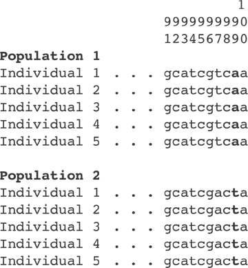
So let us think again about the hypothetical populations we discussed earlier. If it turns out that at least one of the two bases is fixed in the two populations, and is as distinct as shown in figure 2.1, then the ability it confers to diagnose the two populations might be regarded as sufficient for recognizing that the two populations have speciated. And indeed, diagnosis using morphological attributes of organisms is how taxonomy has been done since Carolus Linnaeus invented the science in the mid-eighteenth century.
Figure 2.1 The last ten bases of the genomes of the individuals in the hypothetical populations discussed in the text. The first ninety bases of the genome are identical in all individuals from both populations, and so they are represented by the dots. The numbers above the sequences refer to the positions of the bases in the one hundred base-pair genome. The diagnostic base is the next to last one and is in bold.
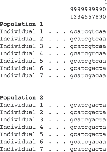
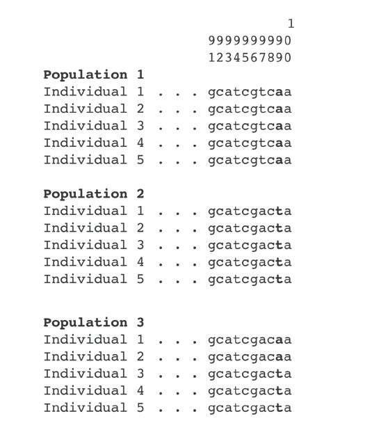
But the diagnostic approach also has its shortcomings. First, the fewer individuals one uses to create the diagnostic, the weaker the conclusion will be. Imagine examining two populations with five individuals in each population and finding a diagnostic that is both fixed and different between the two populations. It is very likely in this case that if you go on a collecting trip a week later and collect two more individuals from each population, the diagnosis will fall apart, because you have collected some new individuals that do not have the diagnostic (figure 2.2). Additionally, if you examine more populations, the diagnostic has a higher likelihood of being destroyed (figure 2.3). And these caveats more than likely apply to any criterion one might derive from a species concept.
Figure 2.2 Increasing sample size has the potential to destroy diagnosis.
Figure 2.3 Increasing the number of populations has the potential to destroy diagnosis.
In this example, the diagnosis was upset by adding more data. Does this mean that the initial diagnosis was invalid when it was made? Actually, no. The inference made at the time the diagnosis was first made was perfectly logical and valid, because all taxonomic conclusions are hypotheses. And, like all scientific hypotheses, they are susceptible to being falsified by more or better data. This example points to an important aspect of systematics and taxonomic science: namely, they are revisionary and subject to constant review. If we had collected all the individuals of the populations concerned, and no other populations were ever found to exist, then revision would not be possible, and the original diagnosis would have to stand. But as long as there are more of the same organisms out there, the possibility of a revised diagnosis—or of additional corroboration of the original one—is always there.
Species, then, may be slippery things; and the packaging of nature, while clearly real in a fundamental sense, is much less tidy than the orderly minds of systematists might like. Nonetheless, we suggest that with the use of appropriate methods, most species, at least in the living world, can be detected with fair confidence. Indeed, it often turns out that diagnosis is a reasonably good proxy for the biological species concept, especially when bolstered by as much other evidence as possible, including that of behavior, ecology, and geographical distributions.
But what about the further subdivision of a species into subspecies, or races? Here we are in very tricky territory indeed, because we can see no objective way to address those hypotheses of subspecific differentiation. At this level the reproductive criterion does not apply, and any other criterion one might attach to the delineation of subspecies or races will be entirely subjective. One distinguished biologist once declared that “subspecies may be recognized if they are useful to the taxonomist,” pretty much conceding that they have no objective existence. Accordingly, in most contexts the terms “subspecies” and “race” are used mostly when a researcher is unsure of the status of a population. In other words, they are generally used in taxonomy as highly provisional hypotheses of species existence. And logically, if one can reject the hypothesis that there is a species boundary in a system, then the hypothesis is discarded and one can move on.
Where does this leave us in the case of Homo sapiens? When Linnaeus named and diagnosed our species back in the eighteenth century, he did it with the enigmatic comment nosce te ipsum, “know thyself.” And though this would normally be rather unhelpful in taxonomic terms, it is no impediment in practice to recognizing the boundaries of our species, because we are the lone surviving twig of what was once a very luxuriantly branching hominid tree. On the outer side, we have no close living relatives who might make a claim on our identity; and on the inner one, it is abundantly clear that we fulfill Mayr’s requirement of interbreeding: something we do liberally whenever populations of different geographic origins meet. Linnaeus himself recognized the geographic divisions Americanus, Europaeus, Asiaticus, and Afer (African) within Homo sapiens; but then, he recognized the entirely imaginary Monstrosus and Ferus as well. So while there is no doubt that there has been some differentiation within our species, as we will see in later chapters, this differentiation is extremely recent, entirely superficial, impossible to reliably diagnose, and has no bearing whatsoever on our reproductive status.