A.1 Aggregate Expenditure and Income
When businesses assess how macroeconomic conditions are likely to shape the demand for their products, they focus on the total amount of goods and services that people want to buy. That is, they focus on aggregate expenditure, which refers to the total amount of goods and services that people want to buy across the whole economy. Let’s dig a little deeper into aggregate expenditure to better understand how it is measured.
Aggregate Expenditure
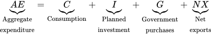
Aggregate expenditure is the sum of four components:
- = Consumption: When households buy goods and services
- + Planned investment: When businesses purchase new capital
- + Government purchases: When the government buys goods and services
- + Net exports: Spending by foreigners on American-made exports, less total spending by Americans on foreign-made imports
Aggregate Expenditure = C + I + G + NX.
Economists often use abbreviations to simplify things, and so you might find it easier to write it this way:
Whichever way you write it, the point is simply that aggregate expenditure is the sum of spending on American-made goods by all economic actors: consumers, businesses, governments, and those engaged in international trade.
Aggregate expenditure includes planned investment, but excludes inventories.

A planned investment.
An unplanned investment.
Notice that aggregate expenditure depends on planned investment, rather than total investment. Let me explain the distinction. Planned investment refers to the investments that a business intentionally makes when it buys capital goods such as buildings, machinery, and software. We use the modifier “planned” to distinguish this from total investment, which—because of an accounting convention—also includes unplanned changes in inventories.
When Ford buys equipment to open a new production line, that’s a planned investment, and it counts as aggregate expenditure. But when Ford can’t sell all the cars it produces, it stockpiles the extra cars as inventories. While accountants classify this increase in inventories as investment, they’re not a planned investment and hence we don’t count them in aggregate expenditure. That’s because when you’re trying to assess economy-wide demand, you want to focus on the stuff that consumers, businesses, and governments purchase, not the unsold inventories they accumulate. Unsold inventories are also the key to seeing the difference between GDP—which measures total output including unplanned investment—and aggregate expenditure.
Now that you know how to measure aggregate expenditure, let’s analyze its key determinant: income.
Aggregate Expenditure Rises with Income
When business analysts forecast aggregate expenditure, they pay special attention to income because it plays an important role in shaping people’s spending decisions. We’re going to follow their lead.
Higher income leads to higher consumption and hence higher aggregate expenditure.
To see why income matters, let’s focus on consumers (like you!). Most people tell me that if their income were higher, they would spend more. If so, then higher individual income leads to higher individual consumption. And because millions of people respond this way, when income across the whole economy is higher—that is, when GDP is higher—then total consumption also tends to be higher.
Figure 1 summarizes this idea with the consumption function, a line plotting the level of consumption associated with each level of income. It illustrates the insight that higher GDP leads to higher total consumption. (You might recognize this idea from Chapter 25 on consumption.)
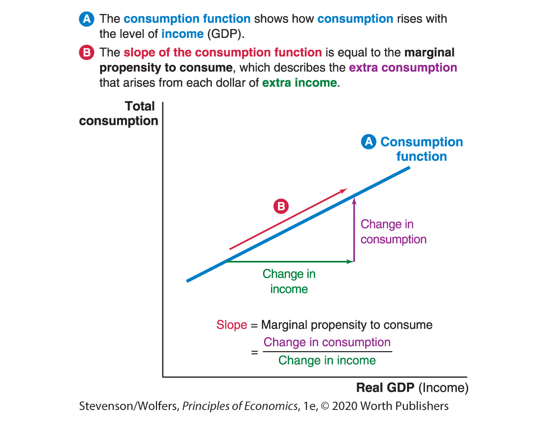
Figure 1 | The Consumption Function
The marginal propensity to consume determines how much consumption rises when income rises.
Typically, when your income rises, you’ll spend a fraction of it today and save the rest. The fraction of each extra dollar of income that a typical household spends is called the marginal propensity to consume (or “MPC,” for short). You can measure the fraction of each dollar someone spends as the ratio of the change in consumption to the change in income. Most people don’t immediately spend all of the extra income they get, suggesting that the marginal propensity to consume is less than one. The slope of the consumption function (remember, slope is “rise over run”) is the ratio of the change in consumption to a change in income. That is, the slope is equal to the marginal propensity to consume.
The marginal propensity to consume is useful because it tells you how much consumption—and hence aggregate expenditure—rises with income. For instance, if the marginal propensity to consume is 0.5, then each extra dollar of income will lead to 50 cents of extra spending this year. It tells the government that if it were to send each American a $100 check in an effort to stimulate the economy, this year’s spending will rise by $50 per person. At the level of the whole economy, it says that if income were to rise by $100 billion, you should forecast consumption will rise by $50 billion.
The aggregate expenditure line shows how aggregate expenditure rises with income.
We now have all the pieces we need to graph the relationship between aggregate expenditure and total income. Let’s start with consumption, and build up from there. The lower line in Figure 2 is the consumption function, which illustrates the tendency for consumption to rise with income (or equivalently, it shows how consumption rises with GDP).
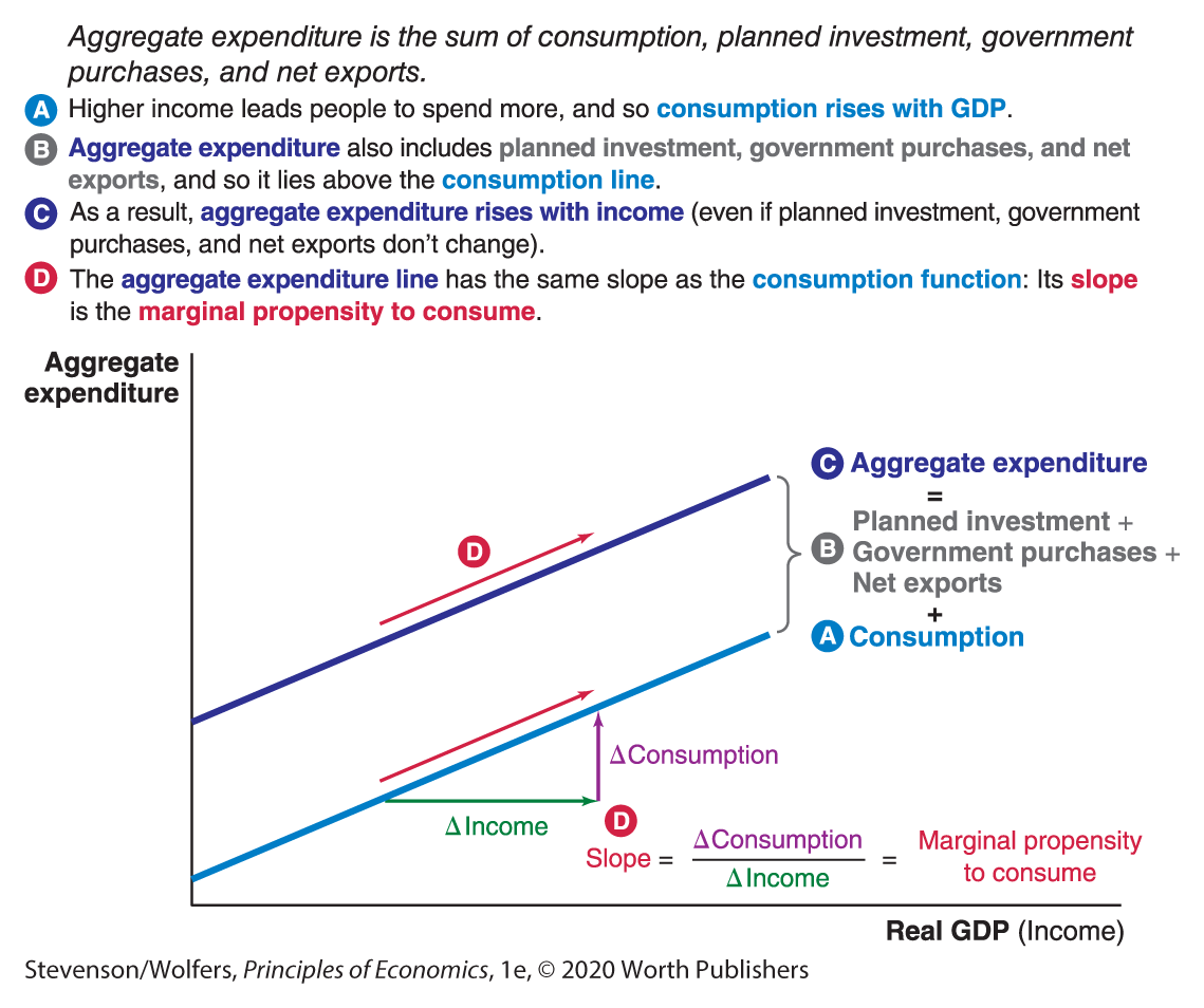
Figure 2 | Aggregate Expenditure Rises with Income
Aggregate expenditure is consumption plus planned investment, government purchases, and net exports. As a result, the aggregate expenditure line lies above the consumption function, and the distance between them is equal to the sum of these other components. If these other components of spending are unaffected by income, then the aggregate expenditure line lies a fixed distance above the consumption function. This means that the slope of the aggregate expenditure line is the same as the slope of the consumption function, and is equal to the marginal propensity to consume. For now, we’re holding planned investment, government purchases, and net exports constant, but in a few pages, we’ll see what happens when they shift.

What fraction do you spend?
How to Use the Aggregate Expenditure Line
The aggregate expenditure line is a valuable tool for managers, and you can use it to assess how robust spending is likely to be next year. For instance, you can forecast what aggregate expenditure will be if total income—that is, GDP—is $18 trillion next year. Figure 3 illustrates how to figure this out. First, locate your GDP forecast on the horizontal axis, then look up until you hit the aggregate expenditure line. Now look across to discover that the corresponding level of aggregate expenditure is $19 trillion.
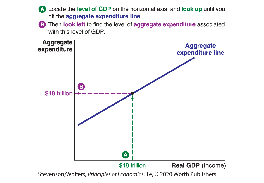
Figure 3 | Use the Aggregate Expenditure Line to Forecast Spending
If other things change, so should your forecast.
Economists often talk about their forecasts as holding other things constant. If other factors change, then so should your forecast. You can use the aggregate expenditure line to forecast the consequences of changing economic conditions. As you do so, it’s important to distinguish between:
- Changes in income, which cause a movement along the aggregate expenditure line; and
- Changes in other factors that change aggregate expenditure at any given income level, which cause the aggregate expenditure line to shift.
Let’s see how this works in practice.
A change in income leads to a movement along the aggregate expenditure line.
What happens when income changes? For instance, what will aggregate expenditure be if GDP rises to $22 trillion?
In Figure 4, locate this new income level on the horizontal axis, and look up until you hit the aggregate expenditure line. Look left, and you’ll see that it corresponds to aggregate expenditure of $21 trillion. You can conclude that increasing income by $4 trillion will lead aggregate expenditure to rise by $2 trillion.
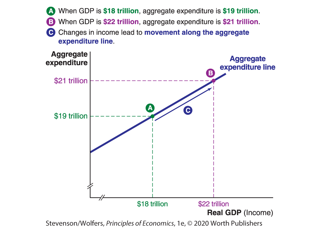
Figure 4 | A Change in Income Causes Movement Along the Aggregate Expenditure Line
Notice that this change in income led spending to move from one point on the aggregate expenditure line to another point on the same line. This makes sense: This line shows how aggregate expenditure responds to a change in income, and so therefore changes in income do not shift this line. Instead, a change in income leads to a movement along the aggregate expenditure line.