A.3 The Multiplier
As the U.S. recession deepened through 2009, newly elected President Obama was desperate to revive the economy. His response was a stimulus bill called the America Reinvestment and Recovery Act, which authorized $787 billion in extra government spending, tax cuts, and other forms of assistance. The goal was to shift the aggregate expenditure line upward, which would stimulate an increase in GDP. It was a big policy change, leading managers everywhere to ask: How will this stimulus affect my business?

Where stimulus goes, will growth follow?
The Multiplier Effect
Caroline owns a construction company in Boston, and she asked her top analysts to evaluate the likely effects of the stimulus for her business. Digging into the details, they noted that the government planned to spend billions of dollars on new construction projects. Caroline immediately directed her staff to look for the best contracts to bid on and to make plans to hire extra workers to work on those projects. Think of this boost as the direct effect of the stimulus.
An initial increase in spending boosts incomes, leading to more spending.
There are also ripple effects. Even though the stimulus contained very little direct spending on cars, economists at Ford still projected it would boost their sales. By their thinking, some of the workers Caroline hired would spend some of their new earnings on new cars. There are also second-round ripple effects. For instance, when Ford hires workers so that it can expand production, some of those new workers will buy lunch at a nearby Subway, leading the franchise owner to hire more sandwich artists. And there are third-round effects, too. If the newly hired sandwich artists spend some of their pay on child care, then local day-care providers will also see higher incomes. And so it continues, showing the power of the interdependence principle, as an initial burst of spending in the construction sector reverberates through the auto, food prep, and child-care sectors, and out to the broader economy.
Add up the ripple effects to find the total effect on GDP.
How far does this process go, and how much does an extra dollar of spending raise GDP? Let’s zoom in and track a single dollar of extra spending as it percolates through the economy.

Beyond the initial impact, there are ripple effects.
Initially, the government spends a dollar, perhaps on a construction contract with Caroline. Then the ripple effects begin. In the first round, the government’s extra spending also counts as extra income for Caroline, and she’ll spend some of it. If her marginal propensity to consume is 0.5, she’ll increase her spending by 0.5 × $1 = 50 cents. There’s a second-round effect: Caroline’s extra spending raises someone else’s income by 50 cents, and they’ll spend a fraction of this extra income. If the typical marginal propensity to consume is 0.5, then Caroline’s spending generates an additional 0.5 × 50 cents = 25 cents of spending. The third-round effects follow the same pattern, with the folks whose income just rose by 25 cents deciding to spend an extra 0.5 × 25 cents = 12.5 cents. And so it goes on, with each further round of ripple effects yielding yet another boost to spending, although these ripples are successively smaller.

Add it all up, and you’ll discover that the initial $1 increase in spending generates a total rise in GDP of: $1 + $0.5 + $0.25 + $0.125 + $0.061 + $0.031 + $0.016 + $0.008 + ⋯ = $2.00.
Don’t get too wrapped up in the math for now (we’ll come back to it). Focus on the bigger picture and you’ll see that a one-dollar increase in aggregate expenditure has a larger effect—a multiplied effect—on GDP. This is a pretty extraordinary insight because it suggests that moderate changes in spending can have much larger macroeconomic effects. This multiplier effect is the reason that many economists believe that the governments can counter large swings in GDP by making moderate changes in the pattern of government purchases that have a multiplied effect offsetting these swings.
The Size of the Multiplier
You can summarize the consequences of a rise in spending—including both the direct impact and the many rounds of subsequent ripple effects—with a single number called the multiplier. The multiplier measures how much GDP changes as a result of both the direct and ripple effects flowing from each extra dollar of spending. In our simple example, the multiplier is 2 because a $1 boost to spending generated a total of $2 in extra GDP.
The multiplier is useful because you can use it to forecast the effects of changes in aggregate expenditure, as follows:

Do the Economics
How much will GDP rise after a new program of renewable energy credits—effectively an incentive for businesses to invest in renewable energy—leads to an additional $100 billion increase in investment in the sector, if the multiplier is 2?


The multiplier is larger if the marginal propensity to consume is larger.
How big is the multiplier in practice? As you’re about to see, it all depends on the marginal propensity to consume (MPC), which you’ll recall is the fraction of each dollar of extra income that gets spent. The MPC matters because the size of each subsequent ripple effect depends on the extent to which extra income translates into extra spending.
To see this, let’s work through the implications of a rise in spending in Figure 9. The initial rise in spending is ΔSpending. In the first-round ripple effect, the recipient of that spending will increase their spending by ΔSpending × MPC. In the second round, the recipient of that extra spending will spend a proportion of it, yielding a further increase in spending of (ΔSpending × MPC) × MPC. In the third round, the recipient of that extra income will increase their spending by (ΔSpending × MPC × MPC) × MPC, and so it goes on.
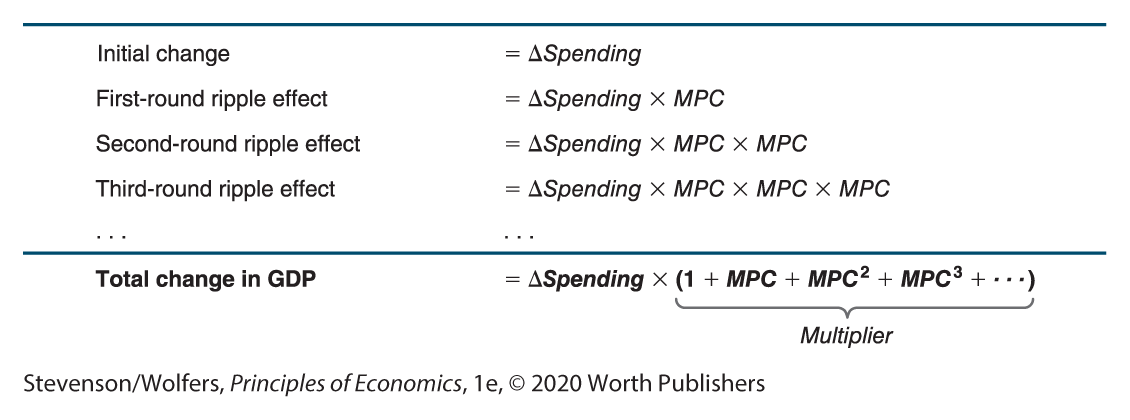
Figure 9 | Multiplier Effects
Add it all up, and you’ll find that the total effect of a rise in spending on GDP is: ΔSpending × (1 + MPC + MPC2 + MPC3 + ⋯), where the expression in brackets is the multiplier. The expression in brackets is the sum of a geometric series, and the beautiful thing is that it all adds up to 1/(1−MPC). That’s it. As a result, the multiplier is equal to:
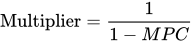
For instance, when the marginal propensity to consume is 0.5, then the multiplier is 1/(1−MPC) = 2. More generally, the larger the marginal propensity to consume, the larger the ripple effects from an initial boost to spending, and hence the larger the multiplier.
EVERYDAY Economics
Beware of developers bearing economic impact studies

Does the multiplier justify using public money to build private stadiums?
The multiplier effect is an important part of macroeconomic analysis, but beware because it’s often misused in microeconomic studies. For instance, every few years a major sports team approaches their city or state government, asking for multimillion dollar subsidies to build a new stadium. They’ll bring with them architectural drawings, and an “economic impact analysis,” in which their highly paid consultants detail the extra spending the stadium will bring. They’ll usually describe massive multiplier effects that suggest the effect on local businesses will be even larger. For instance, when the former Oakland Raiders proposed moving to Las Vegas, they estimated that a new football stadium would stimulate an extra $472 million in annual spending that—due to multiplier effects—would boost output by $786 million per year. The team’s owners used these numbers to convince local legislators to kick in $750 million of taxpayer money to help fund their stadium.
But these analyses often don’t tell the whole story. The first problem is that a new stadium may not boost aggregate expenditure much at all—even if the stadium typically sells out. If you spend $60 more on football tickets, I bet you’ll pay for it partly by spending less on other forms of entertainment. So spending more on football tickets means less spending on other forms of entertainment. The second problem is that the multiplier for a city is typically quite small because spending spills across city borders. For instance, when the newly employed folks at the Nevada Chargers football stadium spend their earnings on food, movies, and technology, they’ll boost the economy of California (where lots of agricultural products, movies, and software are produced), more than Nevada (where the income was earned). Together, these ideas explain why economists have found that stadiums rarely provide much of a boost to the local economy.

The multiplier applies to all increases in spending.
There’s one final thing to note: While we’ve focused on the effects of an increase in government purchases, the multiplier applies with equal force to any increase or decrease in aggregate expenditure. Just as increasing government purchases will have ripple effects, so, too, will changes in consumption, investment, or net exports.
Interpreting the DATA
How big is the multiplier?
Economists have conducted hundreds of studies attempting to answer the question: How big is the multiplier? In most cases they try to assess how effectively fiscal policy—changes in government spending and taxes—can stimulate a weak economy.
This turns out to be a surprisingly difficult question to answer. The problem is that the relationship between government purchases and output reflects (at least) three different forces. The first is the multiplier effect, in which greater government purchases boost future output. The second is called the fiscal policy reaction function, which reflects the reality that policy makers implement fiscal stimulus—increasing government purchases—when they anticipate weaker future output. The third is the monetary policy reaction function, which describes the Federal Reserve’s tendency to cut interest rates when it anticipates weak future output. The multiplier effect creates a link from higher government purchases to higher future output. The fiscal policy reaction function creates a link from lower future output to higher government purchases. And the monetary policy reaction function creates a link from lower future output to lower interest rates, which boosts aggregate expenditure. All of this means that the correlation between government purchases and future output reflects a mishmash of these three forces.
In response, researchers have devised some ingenious studies to measure the multiplier effect. They first isolate and then track the effects of changes in government purchases that aren’t caused by the state of the economy (and hence don’t reflect the fiscal policy reaction function), and that don’t cause the Fed to respond (and hence don’t reflect the monetary policy reaction function). Some studies examine changes in government spending on the military caused by geopolitical tensions, finding that these lead to higher output. Others examine the historical record, finding that changes in tax rates, which were motivated by long-run considerations unrelated to the business cycle, also subsequently boost output. Still others have examined how the funding formulas used in a recent national fiscal stimulus led to a bigger increase in government purchases in some states than in others, finding that those states that received a bigger increase in government spending had a more robust economic recovery.
So, you might ask, what is the multiplier? Figure 10 illustrates an attempt by nonpartisan economists at the Congressional Budget Office to synthesize the available studies. It illustrates three key findings:
- The central estimate—shown in red—is that the multiplier is about 1.5.
- The ripple effects that create the multiplier effect play out over time and may take over a year to become fully evident.
- There is tremendous uncertainty about the multiplier. The top gray line shows the “high estimate,” which is that the multiplier is 2.5. The lower gray line shows the “low estimate,” which is that the multiplier is 0.5. (You might wonder how the multiplier could be less than one. That can occur if extra government spending leads to less spending by consumers and businesses.) In between these high and low estimates is a vast gray expanse, which illustrates that even today, economists don’t think they know the size of the multiplier with any certainty.
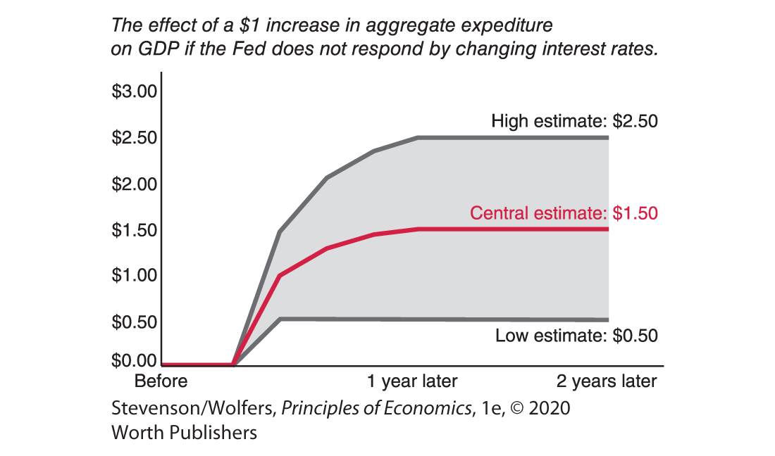
Figure 10 | Estimates of the Multiplier Effect
Data from: Congressional Budget Office.