3.2 Your Decisions and Your Individual Supply Curve
So far, we’ve learned how to summarize your supply plans using an individual supply curve. But where do these plans come from? Let’s step back to see how Shannon prepared her analysis. We’ll start by digging into the best pricing decisions for BP, and then turn to how to use the core principles to guide the choice of what quantity to produce at each price.
Setting Prices in Competitive Markets
A central part of any management role is understanding your competitive environment, and Shannon has analyzed BP’s position carefully. It operates in a fiercely competitive market in which there are dozens and dozens of refineries producing gasoline. Those refineries are all trying to sell their gas through thousands of gas stations around the nation—and the main product they sell—gasoline—is pretty much identical. Consumers are just as happy purchasing gas refined by BP as they are purchasing gas refined by any other firm, because BP gas is neither better nor worse than gas from Exxon, Shell, or Chevron.
Shannon has discovered that BP operates in a market characterized by perfect competition, which is the special case in which 1) all firms in the market are selling an identical good; and 2) there are many sellers and many buyers, each of whom is small relative to the size of the market. This has important implications for BP’s price-setting strategy.
Perfectly competitive firms are price-takers, following the market price.
When you’re operating in a perfectly competitive market, your best strategy is to charge a price that is pretty much identical to whatever your competitors are charging. And so when the prevailing market price of gas is $3 per gallon, Shannon recommends that BP follow along, also selling its gas for around $3.
Here’s why. BP could try charging a bit more than the market price, but if you charge $3.10 when your competitors sell an identical product for $3, you’ll quickly lose all your customers. Alternatively, BP could try to undercut its competitors, selling its gas for $2.90 per gallon, instead. But this doesn’t make sense either. Because BP is small relative to the entire refinery industry, it can expand production and still continue to sell a higher quantity of gas at the market price of $3 per gallon. So the only effect of charging a price below the market price will be to reduce the profits you earn on each gallon of gas you produce.
Consequently, managers in perfectly competitive markets don’t spend a lot of time strategizing about price, because their best price is the market price. This makes them price-takers, which means they take the market price as given and just follow along. Likewise, when you’re a buyer in a perfectly competitive market—say, when you’re buying gas—you’re acting as a price-taker, because you take the price as given, and decide what quantity to buy.
Not all markets are perfectly competitive.
Of course, not all businesses operate in perfectly competitive markets, and so this advice isn’t for everyone. If you operate in a market with only a handful of buyers or a handful of sellers, it’s likely that you can have an important influence on the price. If this describes your industry, we’ll analyze how best to set prices when we learn about market power—a key concept in microeconomics.
But for the rest of this chapter—and indeed, throughout our analysis of supply, demand, and equilibrium—we’ll focus on perfectly competitive markets in which buyers and sellers are price-takers. Partly this is because nearly all markets involve some degree of competition, and so this is a natural foundation on which to build your understanding. We’ll learn how perfectly competitive markets work, and along the way we’ll build the analytical foundation you’ll need when you later turn to focusing on imperfectly competitive markets. It’s also to help simplify your introduction to economics. If all this talk of perfectly and imperfectly competitive markets seems a bit hazy now, don’t worry, stick with microeconomics and we’ll explore it more directly later when we learn about market power. But for now, realize that focusing on price-takers simplifies things, because then you can analyze the question of what quantity to produce separately from the question of what price to set.
Choosing the Best Quantity to Supply
Since BP operates in a perfectly competitive market, Shannon focuses her attention on the question of what quantity to supply at any given price. She has a vast spreadsheet listing information about the costs of producing more or less gas. But how can she transform this information into a concrete plan?
Apply the core principles to your supply decisions.
It’s time to put yourself in Shannon’s shoes and apply the core principles, so that you can figure out the plan that’ll yield the largest possible profit for BP. We’ll start by figuring out what quantity to supply when the price of gas is $3 per gallon. If you repeat this step for the whole range of prices, you will have mapped out BP’s whole supply curve.
So let’s start by analyzing how many gallons of gas BP should produce when the price is $3. I’ve included the core principles in Figure 4 below, to remind you of how they might help you here.
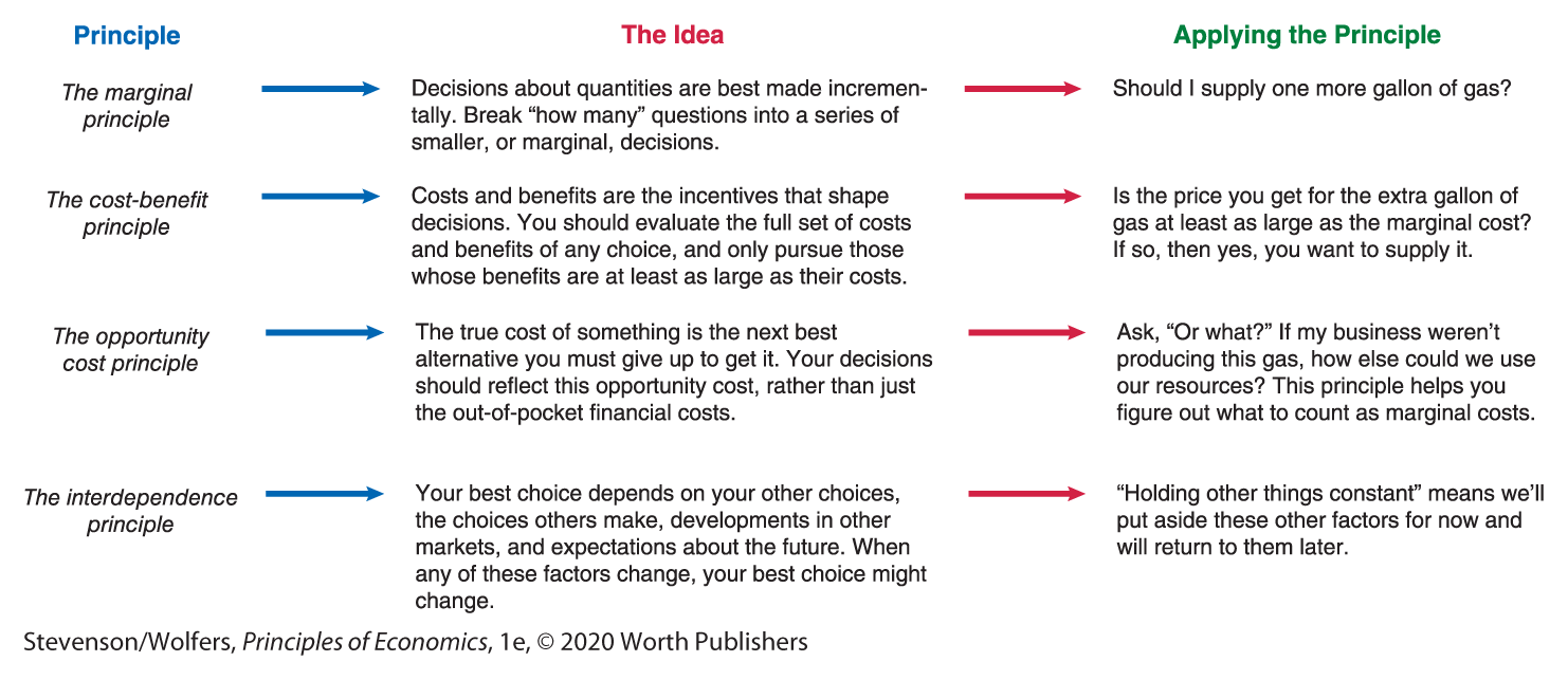
Figure 4 | Applying the Core Economic Principles to Your Supply Decisions
Thinking at the margin means asking: Should you produce one more?
The marginal principle says that decisions about quantities are best made incrementally, and that you should break “how many” questions into a series of smaller marginal choices. Instead of asking “how many” gallons of gas to produce, ask: Should I produce one more gallon of gas?
Compare marginal benefit and marginal cost.
The answer depends on the cost-benefit principle, which says: Yes, you should produce that additional gallon of gas if the benefit of that extra gallon exceeds the cost. That is, your decision depends on the balance of marginal benefits and marginal costs.
Of course, it’s a bit unrealistic to think that a refinery manager who’s responsible for making millions of gallons of gas per day will analyze her production gallon by gallon. She might think instead in terms of whether to expand annual production of gas by a million extra gallons. But we’ll persist in asking whether to produce just one more gallon because it points to the important insight—one confirmed by many leading managers—that smart supply decisions focus on marginal benefits and marginal costs.

Someday, you will learn to love spreadsheets.
The marginal benefit to your firm of producing an additional gallon of gas is simply the amount of money you’ll get for it. If the price of gas is $3, then the marginal benefit to BP of producing another gallon of gas is $3. That is, in a perfectly competitive market, your marginal benefit is the market price.
What about the marginal cost—that is, the extra cost from producing one extra gallon of gas? Turning back to her spreadsheets, Shannon sees that she has detailed data on the quantities of crude oil and other inputs, such as chemical additives, that will be needed in order to expand production, as well as the overtime hours it’ll require.
Your marginal costs include variable costs but exclude fixed costs.
As you think about what expenses to include in your calculation of marginal cost, you should apply the opportunity cost principle, asking “or what?” You shouldn’t just calculate the cost of producing another gallon of gas, you should compare it to the next best alternative, which is not expanding production.
If BP expands production, it’ll have to buy more crude oil, more chemical additives, and pay its workers to work overtime. In the next best alternative—in which BP doesn’t expand production—it won’t need to buy this extra oil, extra chemicals, or pay these extra wages. As such, these are all opportunity costs—they’re costs that BP incurs when it expands production, but wouldn’t incur otherwise. These are called variable costs, because they vary with the quantity of output you produce. Your marginal costs are your additional variable costs.
Shannon’s spreadsheets also show that BP incurs a range of other costs. For instance, there’s the cost of the refinery structures and equipment. But these pose no opportunity cost, because BP would have to pay for its building and equipment even if it pursued its next best alternative of not expanding production. The same is true for the land that it uses and the money BP pays its top managers, because producing another gallon of gas doesn’t require more land or another CEO. These are all examples of fixed costs that don’t change when you vary the quantity of output you produce. Because you have to pay your fixed costs whether or not you expand your production, they’re not part of the opportunity cost of producing more gas. Your fixed costs are irrelevant to your marginal cost.
Bottom line: As you calculate your marginal cost, make sure that it reflects only the variable costs that you’ll incur from producing extra gas, and that you’re excluding all fixed costs.
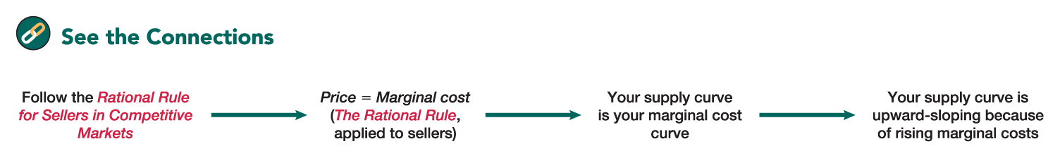
The Rational Rule for Sellers in Competitive Markets
It’s time to put all of this advice together. We’ve worked through the core principles—as summarized in the flowchart below—and that led us to the conclusion that BP should keep selling additional gallons of gas as long as the price is greater than (or equal to) the marginal cost.

In fact you’ve uncovered a pretty powerful rule, which you can apply to any selling decision (in perfectly competitive markets):
The Rational Rule for Sellers in Competitive Markets: Sell one more item if the price is greater than (or equal to) the marginal cost.
The Rational Rule for Sellers puts together the advice from three of the four principles in one sentence. It takes the big question facing managers about what quantity to sell, and reminds you to think at the margin, assessing whether to sell one more item by comparing your marginal benefit (in this case, the price you’ll get) with the marginal cost, recognizing that you should tally up your additional variable costs because they’re the only true opportunity cost of expanding production.
Managers in competitive markets apply this rule to their real-world supply decisions. For instance, it says to Shannon that BP should expand production if the price of gas exceeds marginal cost. Indeed, BP should keep expanding production for as long as the price continues to be at least as large as marginal cost.
Follow the Rational Rule for Sellers to maximize your profits.
The Rational Rule for Sellers is good advice because it’ll lead you to expand production whenever it’ll boost your profits. After all, if the price of that extra gallon of gas exceeds the marginal cost, then producing and selling that extra gallon will lead BP’s revenues to rise by at least as much as their costs. As a result, BP’s profit—which is its revenues minus its costs—will rise. Indeed, if you relentlessly follow the Rational Rule for Sellers—so that you take every opportunity to supply goods when the price is at least as high as your marginal cost—you’ll produce the quantity that earns your firm the largest possible profit. It’s the fact that this rule maximizes your profits that makes it good advice for aspiring managers to follow.
(And if you’re wondering why the Rational Rule for Sellers says to still sell an item even when its price is exactly equal to it marginal cost, realize that doing so will neither increase nor decrease your profits. It says to continue to sell up to, and including, the point when price equals marginal cost, only because it’ll make the rest of your analysis a bit simpler.)
Keep selling until price equals marginal cost.
If you follow this rule consistently, you’ll continue to raise the quantity you supply until the point at which the marginal cost of the last gallon is equal to the price. Why? Just as the Rational Rule for Buyers tells you to keep buying until your marginal benefit is equal to your marginal cost (which is the price), the Rational Rule for Sellers tells you to keep selling gallons of gas until your marginal benefit (the price) is equal to your marginal cost. That means you raise the quantity of gas supplied as long as the price of each additional gallon is at least as high as the marginal cost. Consequently, you should stop increasing the quantity of gas you supply just before the marginal cost exceeds the price—which occurs in competitive markets when the price equals marginal cost.
You might recognize this insight as applying the Rational Rule from Chapter 1, which said: “If something is worth doing, keep doing it until your marginal benefits equal your marginal costs.” When you’re a supplier in a competitive market, the marginal benefit of selling an additional item is the price. As such, adapting the rule to your role as a supplier in a competitive market says you should expand production until:
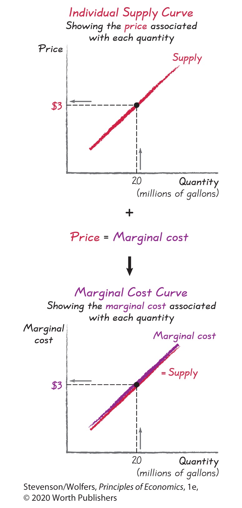
Price = Marginal cost
Your supply curve is also your marginal cost curve.
At this point, it should be clear why economists say that understanding supply is all about understanding marginal costs.
Indeed, this reveals a new perspective for thinking about supply: Your firm’s individual supply curve is also its marginal cost curve. After all, your individual supply curve plots the price associated with each specific quantity of gas you might supply. If you keep selling until price equals marginal cost, then the same curve illustrates the marginal cost associated with each gallon of gas.
Your supply curve reveals your marginal costs.
This yields an important insight. As an executive, you might want to compare your company’s marginal costs to those of your rivals. Or perhaps as an analyst tracking the industry, you might be interested in understanding a business’s cost structure. Or as a policy maker, you might need to better understand the costs of certain activities. You could try asking, but most companies will refuse to divulge this proprietary information, particularly if they’re worried that you’ll use it to gain a competitive edge. But don’t let that stop you. As long as a company follows the Rational Rule for Sellers, its individual supply curve is also its marginal cost curve. And this means that you can also learn about its marginal costs just by observing its selling patterns. For instance, if a rival refinery supplies exactly 20 million gallons of gas when the price is $3, then you can infer that the marginal cost of producing that final gallon must be roughly $3.
Let’s summarize: Supply is all about marginal costs. Indeed, your supply curve is your marginal cost curve. Consequently, understanding supply is really about understanding marginal costs, and this insight sets the stage for the rest of this chapter.
Rising Marginal Cost Explains Why Your Supply Curve Is Upward-Sloping
Recall that the law of supply says that the quantity supplied tends to be higher when the price is higher. That is, it says the supply curve is upward-sloping. But what makes the supply curve upward-sloping?
For companies that follow the Rational Rule for Sellers, the supply curve is also their marginal cost curve. This implies that the supply curve must be upward-sloping because the marginal cost curve is upward-sloping. And why is that? Because, at some point as you increase the quantity you produce, the marginal cost of producing an extra gallon of gas rises. This increasing marginal cost reflects bottlenecks that arise when you try to expand production.
Diminishing marginal product leads to rising marginal costs.
Expanding your production requires increasing your use of inputs, like labor. The extra output you get from an additional unit of input—like hiring one more worker—is called the marginal product of that input. Most firms find that at some point, hiring additional workers yields smaller and smaller increases in output. That is, they experience diminishing marginal product, which occurs when the marginal product of an input declines as you use more of it. (Note that diminishing marginal product doesn’t mean that extra inputs will reduce your output. Rather, it says that the extra output produced by the next worker you hire won’t be quite as large as the extra output produced by the previous worker you hired.)
In the short run, diminishing marginal product can occur when some of your inputs are fixed. Extra workers around a fixed office space can make it crowded and noisy, making it hard for anyone to get anything done. In a factory, extra workers might spend more time waiting for others to finish using equipment. A farmer can sow more seed, but with a fixed plot of land, that’ll lead the plants to become overcrowded and many won’t survive.
In the longer run, you can expand production by increasing all your inputs—hiring more workers, buying more equipment and more land. But the new workers you hire will have less experience and so will take longer to get things done. It’ll be hard to find new land that’s as fertile or well-located as your existing land. Expanding your company’s research and development team won’t boost your output by much if new ideas become harder to find. And managing a large workforce can become more unwieldy, creating coordination problems as your company’s top management is stretched thin. Whatever the cause, the result is that at some point, adding extra inputs won’t produce as much extra output, and so your marginal costs will rise.
EVERYDAY Economics
The diminishing marginal product of homework
You’ve probably experienced diminishing marginal product while writing a paper for a class. The first day’s work might be super productive; you gather your research, put your notes together, and start on a rough draft. On the second day, you expand on a few sections, improve your draft, and work out the inconsistencies. On the third day, you’re starting with a pretty good paper, and while you can find ways to improve it, you’re not making it much better. You could keep working on it forever, and each day you could probably find another small way to improve it. But you’re experiencing diminishing marginal product as the amount that each successive day’s work will boost your grade gets smaller and smaller. At some point the marginal product of an additional day’s work on the paper is so low that you’re better off just handing it in and catching up on your other subjects.

Rising input costs also lead to rising marginal costs.
There’s a second reason why your marginal costs might rise as you increase production: The cost of your inputs might rise. As you buy more of an input, its opportunity cost—what it could be used for instead—rises. You may be required to pay time and a half in order to get your staff to work overtime. Or perhaps you’ll need to offer higher wages to attract more workers. It may also become harder to find workers or other inputs, raising search costs. Or perhaps inputs can only be found farther away, raising transportation costs. The result is that at some point the rising costs of your inputs might lead your marginal costs to rise.
Recap: Individual supply reflects marginal costs.
We’ve come a long way in understanding supply, so let’s take stock. We’ve focused on individual supply—the selling decisions that an individual business makes. We described how an upward-sloping individual supply curve maps out your production plans, summarizing the quantity you will supply at each price.
We then turned to asking: What are the best supply decisions you can make? This led us to the Rational Rule for Sellers in Competitive Markets, and if you follow it, you’ll keep selling until price equals marginal cost. And diminishing marginal product and rising input costs explain why marginal costs are increasing, which explains why businesses are willing to supply a larger quantity only when prices are higher. As a result, supply curves tend to be upward-sloping.
How Realistic Is This Theory of Supply?
By now, you may be scratching your head and asking: Do managers really behave this way? At a large firm like BP, they probably do—graduates with skills like Shannon’s are in high demand, particularly by larger and more sophisticated businesses. But what about other companies?
As sellers experiment, they may come to act as if they follow the core principles.
Many other businesses—particularly smaller businesses—can’t or won’t engage in such deep analytics. But chances are they do something simpler instead. They experiment with the right quantity to produce—producing a bit more or a bit less this week to see how it affects their profits. And this process of experimenting leads their managers to continue to make better decisions, until they’ve eventually discovered the quantity that maximizes their profits. The Rational Rule for Sellers is valuable, because it provides a more direct path to figuring out the quantity that will maximize profits in a competitive market. But ultimately the managers who experiment their way to the profit-maximizing outcome will end up making exactly the same supply choices as if they were following this rule. So if you need to figure out what choices a manager will make, the Rational Rule for Sellers will provide a pretty good forecast.
Survival of the fittest will weed out bad managers.
There’s also an evolutionary force that makes the Rational Rule for Sellers particularly relevant. There are lots of different rules of thumb that a manager could use instead. But many of these alternative rules lead managers to make bad decisions, and their companies eventually go out of business. You can think of this as a version of “survival of the fittest.” The result is that those rules of thumb that lead to decisions that yield outcomes similar to the Rational Rule for Sellers—that is, that get close to maximizing their profits—will survive, while those that yield worse decisions will die out. And so whether intentionally or by accident, the businesses that survive make decisions as if they were following the Rational Rule for Sellers.
Thinking through the principles provides useful advice and helpful forecasts.
The Rational Rule for Sellers is important for two reasons. First, it provides useful advice to you. Managers who understand the rule are successful because it guides them to make the decisions that’ll earn their businesses the largest possible profit. Talk to managers you admire, and you’ll discover that they keep a laser-like focus on their marginal costs when making supply decisions, just as the rule suggests.
It’s also useful for a second reason: If you need to forecast the supply decisions of a savvy manager, it’s a good bet that she or he is thinking through the Rational Rule for Sellers and focusing on marginal costs. And if your competitors or suppliers don’t want to reveal their marginal costs to you, you can still infer what they are by analyzing their supply decisions. Since their individual supply curve is their marginal cost curve, their supply decisions reveal their marginal costs. This is going to be a useful insight as we turn to analyzing how sellers as a group combine to shape market supply.