5.1 Price Elasticity of Demand
The law of demand tells us that when the price falls, the quantity demanded will rise. But as Southwest’s savvy strategists understand, the important question is: By how much? Whether cutting the price of airline tickets leads to a lot more customers, or only a few more, determines whether or not Southwest’s low-fare strategy is a good one. It all depends on how responsive buyers are to prices. That’s why our first task is to figure out how to measure this responsiveness.
Measuring Responsiveness of Demand
The price elasticity of demand measures how responsive buyers are to price changes. Specifically, it measures by what percent the quantity demanded will change in response to a 1% price change.
To measure the price elasticity of demand, observe how the quantity demanded responds to a price change. That responsiveness is measured by the ratio of the percent change in quantity demanded to the percent change in price as you move along the demand curve. That is:

For example, cutting the price of gas by 20% typically leads to an increase in the quantity demanded of about 10%. Putting these numbers together reveals that the price elasticity of gas is about −0.5 (= 10% rise in thequantity demanded/20% fall in the price = 10%/−20%). Notice that the price elasticity of demand is a negative number because cutting the price raises the quantity demanded. In fact, when it comes to movements along the demand curve, the law of demand tells us that price and quantity changes always move in the opposite direction: When the price goes up, the quantity demanded goes down, and when the price goes down, the quantity demanded goes up.
Absolute value focuses on the magnitude of the price elasticity of demand.
Economists often want to focus on the magnitude of the price elasticity of demand. To do this, they use what mathematicians call the absolute value, which simply means ignore the negative sign. Thus, the absolute value of the price elasticity of demand is the price elasticity of demand with the negative sign dropped. It can be expressed using the absolute value symbol, which is two straight lines: 


Do the Economics
When Uber cut the price of a ride in New York City by 15%, it found that the quantity of rides demanded rose by 30%. What is the absolute value of the price elasticity of demand for Uber rides?


When quantity is very responsive, demand is elastic.
What Uber found was that riders were very responsive to prices. When it cut prices, the quantity of rides demanded rose by an even greater percentage. When buyers are very responsive to price, economists describe their demand as elastic. Specifically, we say that demand is elastic whenever the absolute value of the percent change in quantity demanded is larger than the absolute value of the percent change in price. This also means that the absolute value of the price elasticity of demand is greater than 1.
When demand is elastic, price increases also lead to large changes in the quantity demanded. Take Matilda, for example; she lives and works in a small city where she can walk to work. But she prefers to drive to the grocery store. And she likes to take road trips on the weekend, to go hiking in a national park, or to spend a day at the beach four hours away. When the price of gas rises, however, the cost of that day at the beach becomes a bit too high, and when the price of gas goes even higher, those other road trips start to look pretty expensive, too. After all, she can hang out with friends that live close by, go for a run in her neighborhood, or go for a swim at the community pool. All of this means that when the price of gas increases, the quantity of gas Matilda demands falls by a lot.
When quantity is very unresponsive, demand is inelastic.
Oliver lives in a dense city where he can walk, ride a bike, or take public transportation to most of the places he wants to go. However, he needs his car to get to his job in the suburbs. He doesn’t use it for much else. When the price of gas rises, he doesn’t have much choice but to keep buying gas to get to work, and when the price falls, he doesn’t feel the need to drive anywhere else. As such, the quantity of gas Oliver demands is not very responsive to changes in price.
When buyers are not very responsive to price changes, economists describe their demand as inelastic. Specifically, we say that demand is inelastic whenever the absolute value of the percent change in quantity demanded is smaller than the absolute value of the percent change in price. This also means that the absolute value of the price elasticity of demand is smaller than 1.
When the absolute value of the price elasticity of demand is exactly equal to 1 it is neither elastic nor inelastic. Some economists refer to this as unit elastic, so that it has a name. But the important thing to note is simply that this is the dividing line between elastic and inelastic.
Elastic demand curves are relatively flatter than inelastic demand curves.
Figure 1 shows an example of both an inelastic demand curve like Oliver’s (in purple), as well as an elastic demand curve like Matilda’s (in green). One of the first things you might notice is that an elastic demand curve is relatively flat, while an inelastic demand curve is relatively steep. Whenever two demand curves pass through the same point, the demand curve that’s flatter at that point is the more elastic demand curve. This is because when demand is elastic, the quantity demanded is relatively responsive. In contrast, when demand is inelastic, the quantity demanded is relatively unresponsive.
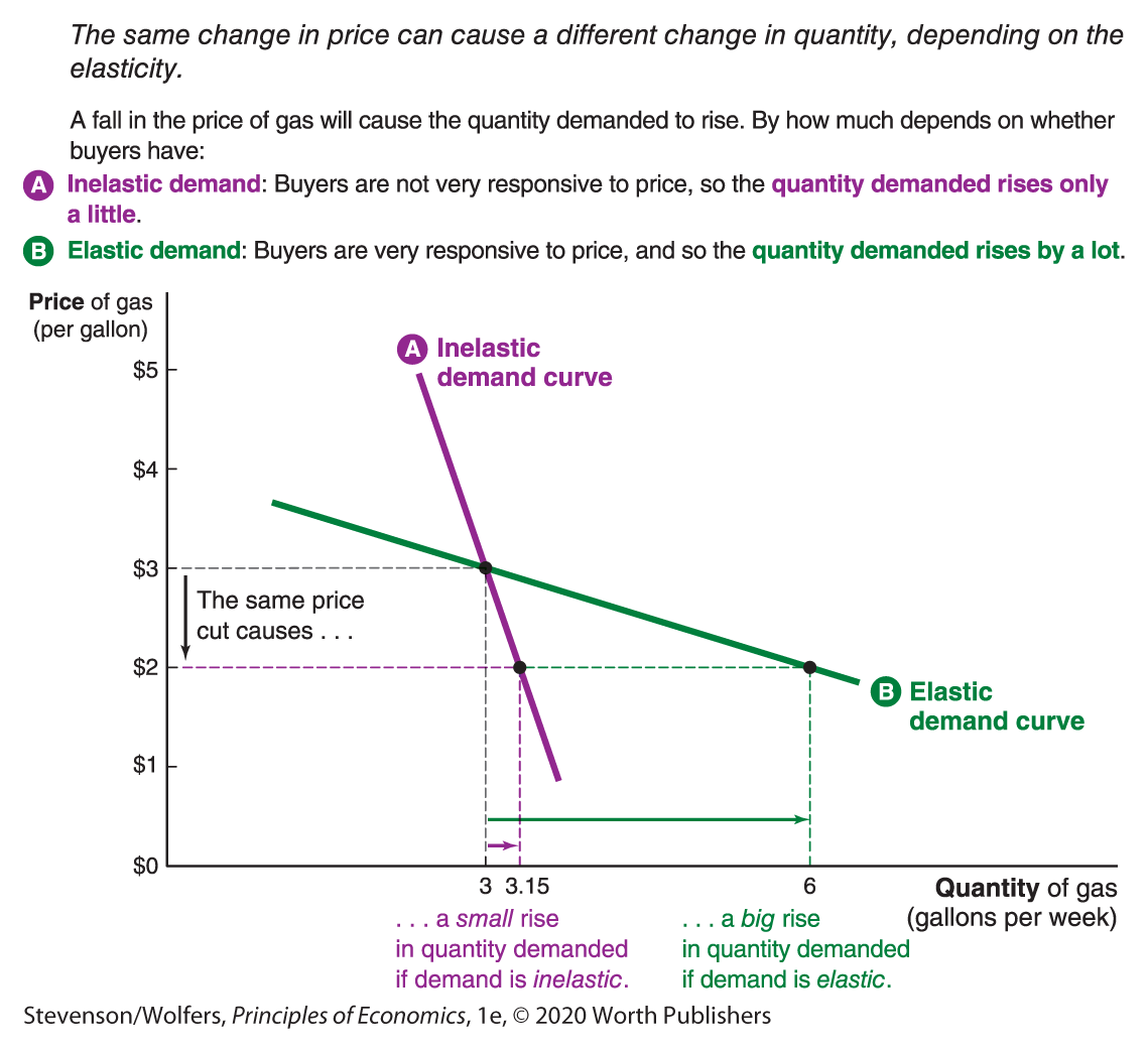
Figure 1 | Price Elasticity of Demand
It’s important to note that elasticity is not, however, the same thing as slope. The slope of the demand curve—remember, slope is rise over run—is equal to the change in price divided by the change in quantity. Elasticity is given by the percent change in quantity divided by the percent change in price. As a result, while linear demand curves, like the one shown in Figure 1, have the same slope all along the curve, the elasticity will differ along the curve.
There are two extreme cases when the slope clearly reveals elasticity. When the demand curve is completely horizontal it means that the price elasticity of demand is infinite—any change in price leads to an infinite change in quantity. Economists call this perfectly elastic demand. When the demand curve is completely vertical it means that the price elasticity of demand is zero—no matter what the change in price, the total quantity demanded is unchanged. Economists call this perfectly inelastic demand.
Interpreting the DATA
Why the minimum wage debate is all about elasticity
In 2019, the federal minimum wage—the lowest wage that you can legally pay most workers—was $7.25 per hour. A proposal to raise the minimum wage to $12 per hour generated a lot of debate; you may have strong opinions on it yourself. Labor activists argue that higher wages will help the poor by helping them earn more. On the other side, business lobbyists argue that a higher minimum wage will hurt the poor by causing employers to employ fewer low-wage workers. Much of this debate is about the price elasticity of demand for labor.
To understand the importance of the price elasticity of demand, you must first realize that in the labor market workers are suppliers who supply their labor. Employers are therefore buyers, who demand the labor of workers. What’s the price employers pay? The wage. So an increase in the minimum wage is an increase in the price that buyers of minimum wage labor must pay. The price elasticity of demand therefore tells us how much the quantity of labor demanded will change when there is an increase in its price.
Some who argue against raising the minimum wage claim that it would cause employers to fire millions of workers. This argument boils down to saying that employer’s demand for labor is very elastic. If this is true, a modest rise in the price of labor (remember, the price of labor is the wage!) leads to a large decline in the quantity of labor demanded. In this case, getting higher wages for the lucky few who still have jobs may not be worth the cost of losing so many jobs (and some even say that it won’t cost any jobs).

Would this be good or bad for low-wage workers?
By contrast, many of those arguing for a higher minimum wage believe that very few people would lose their jobs. They’re claiming that the quantity of labor demanded would not respond much to a higher minimum wage—in other words, that labor demand is very inelastic. By this view, raising the minimum wage will lead to the loss of a small number of jobs.
So the minimum wage debate isn’t simply about being for or against workers. Whether you think it is a good idea to raise the minimum wage will partly depend on whether you think the demand for labor is elastic or inelastic. Did you know you were arguing about elasticity? What are your thoughts? Do you think the demand for labor at a wage of $7.25 per hour is elastic or inelastic? Your answer to that question may be your best guide to deciding whether you support raising the minimum wage.

Recap: The spectrum from perfectly inelastic to perfectly elastic demand.
Figure 2 summarizes the difference between perfectly inelastic, inelastic, elastic, and perfectly elastic demand. As you read through this table, test yourself on what each of these concepts means.

Figure 2 | Inelastic and Elastic Demand
Determinants of the Price Elasticity of Demand
You now know that demand for some goods and services (including the demand for workers) may respond a lot or a little (or somewhere in between) to price changes. And you know that the price elasticity of demand measures this responsiveness. Perhaps you are wondering why the responsiveness of demand to price changes is high for some products and low for others.
Recall that the opportunity cost principle tells you that to figure out the benefits of buying something, you need to compare it to the next best alternative. It follows that price elasticity of demand is all about how good that next best alternative is—in other words, it reflects the extent to which there are good substitutes available for the marginal purchase.
Elasticity is all about substitutability.
Recall that Oliver has inelastic demand for gas, because he has no alternative way to get to work other than driving. Since he doesn’t have a good substitute available, his marginal benefit from the gallons of gas necessary to get to work is very high, and so he will continue to buy enough gas for his commute even if the price rises sharply.
Oliver derives little benefit from other uses of gas. In fact, parking is such a hassle in his neighborhood that once he’s found a spot on Friday after work, he doesn’t want to move his car again until he leaves for work on Monday morning. For Oliver, driving is not a good substitute for walking, and so even if the price of gas falls sharply, it won’t induce him to buy more.
Because Oliver doesn’t have close substitutes for his transportation choices, Oliver’s marginal benefit from the last gallon of gas he consumes—the one that gets him home from work on Friday—is quite high, but the marginal benefit he gets from the next gallon is pretty low. As a result, if the price were to fall or rise, he’s unlikely to change the quantity he demands by much, if at all. Thus, Oliver’s demand for gas is inelastic.
Matilda, on the other hand, has a lot of good substitutes for her current uses of gas. When the price of gas rises, she realizes that hanging out with her friends in town is a pretty good substitute for driving four hours to spend the weekend at the beach, so she will cut back on her gas purchases. Similarly, when the price of gas falls, she is more likely to find that driving for an extra weekend away will pass the cost-benefit test, and so she’ll increase the quantity of gas she purchases. When you are close to indifferent between two options—like Matilda is—small differences in the price can lead you to make very different choices. Thus, Matilda’s demand for gas is elastic.
Bottom line: The availability of substitutes determines the price elasticity of demand. We’ll now take a look at five determinants of the price elasticity of demand, but you’ll quickly see that these determinants are simply factors that help explain what kind of substitutes you are likely to have.
Demand elasticity factor one: More competing products mean greater elasticity.

A lot of competing products.
The more competing products there are, the more likely you are to find a close substitute. As a result, you’ll be more price sensitive when you are shopping at a Walmart Supercenter than at a small corner store. Why? A typical Walmart Supercenter stocks roughly 150,000 different goods. All of those different products mean that you’ll be more likely to find a good substitute if the price of your first choice has gone up. So if the price of Quilted Northern Ultra Plush Double Roll Bath Tissue rises, you might buy Charmin Ultra Strong Mega Roll toilet paper instead. But when you are at the corner store, your only other option might be Scott single-ply toilet paper. Because the Charmin is a closer substitute to the Quilted Northern, a small rise in the price of Quilted Northern will lead more people to make the switch at Walmart than at the corner store.

Fewer competing products.
As you think about competing products, remember to think broadly. For instance, managers at Southwest know that demand is more elastic when their customers have the option of flying on United or Delta instead. But they have also discovered that the demand for flights is more elastic in airports that are near Amtrak train stations, because taking the train is a substitute for flying. They’ve also found that demand is more elastic for shorter flights, for which driving is a reasonable substitute.
Demand elasticity factor two: Specific brands tend to have more elastic demand than categories of goods.

There are plenty of substitute cereals—if you’re willing to accept a substitute.
Because specific brands tend to have more close substitutes, demand for these goods is typically more elastic than demand for broad categories of goods. For example, there are many close substitutes for Honey Nut Cheerios, and so when the price goes up many people will substitute to a different breakfast cereal (or other breakfast item). As a result, demand for Honey Nut Cheerios is quite elastic. By contrast, consumers are less responsive to price changes in the overall category of breakfast cereals. Demand is less elastic because the alternatives—eating something other than cereal, such as yogurt or toast—are quite different.
Demand elasticity factor three: Necessities have less elastic demand.
Things that you really can’t do without are things that you will keep buying even as the price rises. What makes something a necessity? A necessity is something where there isn’t a good substitute available and doing without isn’t a good option. Food is a necessity. What is the alternative to food? To go hungry. That’s not a viable alternative, and it helps explain why demand is inelastic for food staples like eggs, rice, pasta, fruits, and vegetables. Restaurant meals, however, are not a necessity for most people. Why? Because eating at home is a good substitute. Not surprisingly, Figure 3 shows that restaurant meals have more elastic demand than staple foods you might eat at home. However, what’s a necessity for one person might not be for another. For example, if you don’t have access to a kitchen, restaurant meals might be more of a necessity for you.

Figure 3 | Price Elasticity of Demand for Consumer Goods
Demand elasticity factor four: Consumer search makes demand more elastic.
When consumers are willing to search a lot for a low-cost alternative for something, demand for that product is more elastic. Why? Because the more you search for a good deal, the more likely you are to find an acceptable, lower-priced substitute. If stores raise their price, customers actively searching are more likely to find a good alternative. Therefore, those who are most willing to search will be more responsive to price changes.
EVERYDAY Economics
Should you search harder for bargains on perishable or storable goods?
Should you spend more time looking for bargains on perishable goods like fresh fish, or storable goods like laundry detergent? The answer is storable goods. Think about it: If you get a $1 discount on fish, then you can save a dollar on tonight’s dinner. But if you find laundry detergent that is $1 cheaper, you can stock up, buying half a dozen bottles of detergent. Sure, it’ll be enough to last you for months, but buying six bottles means that you’ll save $6 instead of $1.
Since customers tend to stock up when they see a good price on a storable good, demand for storable goods tends to be much more elastic than for perishable goods. And this is still due to substitutability: Today’s low price on detergent is a substitute not just for buying it at a higher price today, but also for buying detergent next month.
Demand elasticity factor five: Demand gets more elastic over time.
On any given day, many of your decisions about what to purchase are difficult to change. For instance, if you take a road trip and the price of gas goes up when you are headed home, you’re probably going to buy the gas you need to get home regardless of any price rise (even if it’s large!). You might buy less gas once you get back home, but you’ll still face constraints like needing to get to work or owning a car that isn’t very fuel-efficient. In the very short run, it’s hard to change how much gas you buy.
But if gas prices stay higher, you’ll adjust your plans over time so you drive even less. You might figure out public transit options. Eventually, you may replace your car with a more fuel-efficient one. You may even consider moving closer to work or school so that you can drive less. And so over time, the same price change will lead to a bigger change in the quantity demanded. This happens because as time passes, you will tend to have more options to choose from, which is another way of saying that more substitutes become available. More substitutes mean more elastic demand, so over time, demand tends to become more elastic. As a result, demand is more elastic in the long run than in the short run. But how long is the long run? It depends on when more substitutes become available. If you were already planning to upgrade your car next month, the long run for you is a month. But for someone locked into a two-year lease on a car, the long run may be two years.
Elasticity will differ by person, product, and price.
All of the factors affecting the price elasticity of demand boil down to whether there are good substitutes for what you want to buy. We described Honey Nut Cheerios as having a lot of close substitutes because most people find that switching to another breakfast cereal doesn’t make them that much less happy. But if you really love Honey Nut Cheerios more than any other breakfast food, then there may not be close substitutes available for you. Your preferences across the available alternatives determine your elasticity of demand. Ultimately, elasticity varies according to who you are, what product you’re considering, what the price is, and how quickly you need to respond.
Your price elasticity of demand also differs depending on where you are on your demand curve. For instance, if you need to drive to go to work, but you like to drive on the weekends as well, then you might have highly inelastic demand when prices are high and you are only buying gas to get to work. But if prices fall enough, your demand might become more elastic as you start buying gas for leisure trips outside of work.
Even though elasticities differ across people, products, and prices, they can be compared because they’re all measuring the same thing: how responsive the percent change in quantity demanded is relative to the percent change in the price.
Do the Economics
Do you think demand is elastic or inelastic for the following goods?
- Flowers on Valentine’s Day
- Health care
- Lay’s potato chips
- Electricity
- Apple iPads

Calculating the Price Elasticity of Demand
So far, you have seen that to measure elasticity, you need the percent change in quantity demanded and the percent change in price. With these two numbers, you are easily able to calculate the price elasticity of demand by dividing the percent change in quantity demanded by the percent change in price.
But what if you need to calculate the percent change in quantity demanded and the percent change in price? It seems easy enough, but you’ll quickly notice an annoying problem—the normal way you think about calculating the percent change depends on where you start. For instance, when quantity goes from 100 to 150, it’s a 50% increase. But if it goes back from 150 to 100 it’s a 33% decrease. That’s an annoying problem because if the percent change depends on the starting point, then elasticity will depend on the starting point. Since we want a consistent measure of elasticity between two points, we need a measure that doesn’t depend on the starting point.
The problem isn’t related to elasticity, but rather how we calculate the percent change in price and quantity. Economists often use a special method called the midpoint formula which measures the percent change between any two points relative to a baseline midway between those two points. Let’s see how we calculate it.
Use the midpoint formula to calculate the percent changes in price and quantity.
To calculate the percent change in quantity between any two points, 

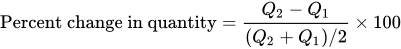

I’m sorry I couldn’t afford flowers this Valentine’s Day; they were too expensive. Please be mine?
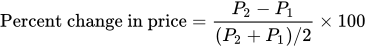
Similarly, to calculate the percent change in price between any two prices, divide the difference between them by the average of the two price points. Thus the midpoint formula for calculating the percent change in price is:
Once you have calculated the percent change in quantity demanded and percent change in price using the midpoint formula, you are ready to calculate the price elasticity of demand given what you already know—it is simply the percent change in quantity demanded divided by the percent change in price.
There’s a bit of math involved with the midpoint formula. So when you’re trying to calculate an elasticity using the midpoint formula, a calculator can come in handy. And because economists don’t always use the midpoint formula, we’ll try to be clear about when we want you to use it.
Do the Economics
The New York City Parks Department learned an important lesson about elasticity when it decided to increase the price of using city-owned tennis courts. Residents used to pay $100 for a seasonal permit, which allowed them to play on any city-owned court. City managers figured that if they raised the price to $200, they would sell nearly as many permits, while increasing their revenue. However, the price increase led the quantity of permits demanded to drop from 12,774 down to 7,265. Calculate the absolute value of the price elasticity of demand for New York tennis permits using the midpoint formula.
Step one: What was the percent change in the price?

Step two: How much did the quantity demanded change as a percent, in response?

Step three: Calculate the elasticity:

Now that you know how to calculate the price elasticity of demand, let’s turn to understanding how you will use it.